Tailoring optical nonlinearities via the Purcell effect

Abstract

We predict that the effective nonlinear optical susceptibility can be tailored using the Purcell effect. While this is a general physical principle that applies to a wide variety of nonlinearities, we specifically investigate the Kerr nonlinearity. We show theoretically that using the Purcell effect for frequencies close to an atomic resonance can substantially influence the resultant Kerr nonlinearity for light of all (even highly detuned) frequencies. For example, in realistic physical systems, enhancement of the Kerr coefficient by one to two orders of magnitude could be achieved.

Optical nonlinearities have fascinated physicists for many decades because of the variety of intriguing phenomena that they display, such as frequency mixing, supercontinuum generation, and optical solitons Drazin:89 ; Boyd:92 . Moreover, they enable numerous important applications such as higher-harmonic generation and optical signal processing Boyd:92 ; Nielsen:00 ; Agrawal:01 . On a different note, the Purcell effect has given rise to an entire field based on studying how complex dielectric environments can strongly enhance or suppress spontaneous emission from a dipole source Purcell:46 ; Kleppner:81 ; Ryu:03 ; Bermel:04 ; Englund:05 . In this Letter, we demonstrate that the Purcell effect can also be used to tailor the effective nonlinear optical susceptibility. While this is a general physical principle that applies to a wide variety of nonlinearities, we specifically investigate the Kerr nonlinearity, in which the refractive index is shifted by an amount proportional to intensity. This effect occurs in most materials, modeled here as originating from the presence of a collection of two-level systems. We show theoretically that using the Purcell effect for frequencies close to an atomic resonance can substantially influence the resultant Kerr nonlinearity for light of all (even highly detuned) frequencies.

In hindsight, the modification of nonlinearities through the Purcell effect could be expected intuitively: optical nonlinearities are caused by atomic resonances, hence varying their strengths should influence the strengths of nonlinearities as well. Nevertheless, to the best of our knowledge, this interesting phenomenon has not thus far been described in the literature. Moreover, as we show below, it displays some unexpected properties. For example, while increasing spontaneous emission strengthens the resonance by enhancing the interaction with the optical field, it actually makes the optical nonlinearity weaker. Furthermore, phase damping (e.g., through elastic scattering of phonons), which is detrimental to most optical processes, plays an essential role in this scheme, because in its absence, these effects disappear.

A simple, generic model displaying Kerr nonlinearity is a two-level system. Its susceptibility has been calculated to all orders in both perturbative and steady state limits Boyd:92 . However, this derivation is based on a phenomenological model of decay observed in a homogeneous medium, and does not necessarily apply to systems in which the density of states is strongly modified, such as a cavity or a photonic crystal bandgap. Following an approach similar to Ref. JohnQu:96, , the validity of this expression can be established from a more fundamental point of view. Start by considering a collection of $N$ two-level systems per unit volume in a photonic crystal cavity, whose levels are labeled $a$ and $b$. The corresponding Hamiltonian is given by the sum of the self-energy and interaction terms ($H_{0}$ and $V(t)$, respectively). Using the electric dipole approximation, one obtains:

$$H=H_{0}+V(t)=\hbar\left[\omega_{a}\sigma_{aa}+\omega_{b}\sigma_{bb}+\Omega(t)\sigma_{ab}+\Omega^{*}(t)\sigma_{ba}\right],$$ (1)

where $\sigma_{ij}=c_{i}^{\dagger}c_{j}$ is the operator that transforms the fermionic state $j$ to the fermionic state $i$, $\Omega(t)=-\vec{\mu}\cdot\vec{E}(t)/\hbar$ is the Rabi amplitude of the applied field as a function of time, and the scalar dipole moment $\mu$ is defined in terms of its projection along the applied field $\vec{E}(t)$. In general, if this system is weakly coupled to the environmental degrees of freedom, then the timescale for the observable dynamics of the system is less than the timescale of the “memory” of the environment. In this case, information sent into the environment is irretrievably lost – this is known as the Markovian approximation Preskill:04 . The dynamics of this system can then be modeled by the Lindbladian ${\cal L}$, which is a superoperator defined by $\dot{\rho}\equiv{\cal L}\left[\rho\right]$. In general, one obtains the following master equation from the Lindbladian:

$$\dot{\rho}=-(i/\hbar)\left[H,\rho\right]+\sum_{\mu}\left[L_{\mu}\rho L_{\mu}^{\dagger}-\frac{1}{2}L_{\mu}^{\dagger}L_{\mu}\rho-\frac{1}{2}\rho L_{\mu}^{\dagger}L_{\mu}\right]$$ (2)

Using the only two quantum jump operators that are allowed in this system on physical grounds – $L_{1}\equiv\sigma_{ab}/\sqrt{T_{1}}$ and $L_{2}\equiv\sigma_{bb}\sqrt{\gamma_{\mbox{\tiny phase}}}$ Preskill:04 – one can obtain the following dynamical equations:

$$\frac{d\rho_{ba}}{dt}=-(i\omega_{ba}+T_{2}^{-1})\rho_{ba}+i\Omega(t)(\rho_{bb}-\rho_{aa})$$ (3)

$$\frac{d(\rho_{bb}-\rho_{aa})}{dt}=-\frac{(\rho_{bb}-\rho_{aa})+1}{T_{1}}-2i\left[\Omega(t)\rho_{ab}-\Omega^{*}(t)\rho_{ba}\right],$$ (4)

where $\omega_{ba}\equiv\omega_{b}-\omega_{a}$, $T_{1}$ is the rate of population loss of the upper level, and $T_{2}=(1/2)T_{1}^{-1}+\gamma_{\mbox{\tiny phase}}$ is the rate of polarization loss for the off-diagonal matrix elements. The prediction of exponential decay via spontaneous emission is known as the Wigner-Weisskopf approximation CohenTannoudji:77 . Although it has been shown that the atomic population can display unusual oscillatory behavior in the immediate vicinity of the photonic band edge John:94 ; Lambropoulos:00 , theoretical JohnQu:96 and experimental considerations Bayer:01 ; Lodahl:04 show that this approximation is fine for resonant frequencies well inside the photonic bandgap. In the rest of this manuscript, this is assumed to be the case. Next, one can make the rotating wave approximation for Eqs. (3) and (4), and then solve for the steady state. If the polarization is defined by $P=N\mu(\rho_{ba}+\rho_{ab})=\chi E$, where $\chi$ is the total susceptibility to all orders, one obtains the following well-known expression for the susceptibility Boyd:92 ; JohnQu:96 :

$$\chi=-\frac{N\mu^{2}(\omega-\omega_{ba}-i/T_{2})T_{2}^{2}/\hbar}{1+(\omega-\omega_{ba})^{2}T_{2}^{2}+(4/\hbar^{2})\mu^{2}|E|^{2}T_{1}T_{2}}.$$ (5)

In general, equation (5) may be expanded in powers of the electric field squared. Of particular interest is the Kerr susceptibility, also in Ref. Boyd:92, :

$$\chi^{(3)}=\frac{4}{3}N\mu^{4}\frac{T_{1}T_{2}^{2}(\Delta T_{2}-i)}{\hbar^{3}(1+\Delta^{2}T_{2}^{2})^{2}},$$ (6)

where $\Delta\equiv\omega-\omega_{ba}$ is the detuning of the incoming wave from the electronic resonance frequency. For large detunings $\Delta T_{2}\gg 1$, one obtains the approximation that:

$$\mbox{Re}\,\chi^{(3)}\approx\frac{4}{3}N\mu^{4}\left(\frac{1}{\hbar\Delta}\right)^{3}\frac{T_{1}}{T_{2}}.$$ (7)

Of course, there are many types of materials to which a simple model of noninteracting two-level systems does not apply. However, it has been shown that some semiconductors such as InSb (a III-V direct bandgap material) can be treated as a collection of independent two-level systems with energies given by the conduction and valence bands, and yield reasonable agreement with experiment Miller:80 . If the parameter $\Delta$ is defined in terms of the bandgap energy such that $\Delta\equiv\omega_{G}-\omega$, then one can look at the regime $\Delta T_{2}\gg 1$ studied above, and obtain the following equation:

$$\mbox{Re}\,\chi^{(3)}\approx-\frac{1}{30\pi\hbar^{3}}\left(\frac{eP}{\hbar\omega}\right)^{4}\left(\frac{2m_{r}}{\hbar\Delta}\right)^{3/2}\frac{T_{1}}{T_{2}},$$ (8)

where $P$ is a matrix element discussed in Ref. Miller:80, , $\omega_{G}$ is the direct bandgap energy of the system, and $m_{r}$ is the reduced effective mass of the exciton. This equation displays the same scaling with lifetimes as Eq. (7), so the considerations that follow should also apply for such semiconductors.

Now, consider the effects of changing the spontaneous emission properties for systems modeled by Eqs. (7) or (8). When spontaneous emission is suppressed, as in the photonic bandgap of a photonic crystal, $T_{1}$ will become large while $T_{2}$ remains finite, thus enhancing $\chi^{(3)}$ by up to one or more orders of magnitude (for materials with the correct properties). For large detunings (where $\Delta T_{2,\mbox{\tiny vac}}\gg 1$), we expect that $\chi^{(3)}$ will scale as $T_{1}/T_{2}$. The enhancement of the real part of $\chi^{(3)}$ is defined to be $\eta\equiv\mbox{Re}\,\chi^{(3)}_{\mbox{\tiny purcell}}\,/\,\mbox{Re}\,\chi^{(3)}_{\mbox{\tiny hom}}$, where $\chi^{(3)}_{\mbox{\tiny purcell}}$ is the nonlinear susceptibility in the presence of the Purcell effect, while $\chi^{(3)}_{\mbox{\tiny hom}}$ is the nonlinear susceptibility in a homogeneous medium. Since $T_{1}^{-1}=\Gamma_{\mbox{\tiny rad}}+\Gamma_{\mbox{\tiny nr}}$, the maximum enhancement is predicted to be roughly:

$$\eta\approx\frac{T_{1,\mbox{\tiny purcell}}T_{2,\mbox{\tiny vac}}}{T_{1,\mbox{\tiny hom}}T_{2,\mbox{\tiny purcell}}}=\frac{\frac{1}{2}\Gamma_{\mbox{\tiny nr}}+\gamma_{\mbox{\tiny phase}}}{\frac{1}{2}(\Gamma_{\mbox{\tiny nr}}+\Gamma_{\mbox{\tiny rad}})+\gamma_{\mbox{\tiny phase}}}\frac{\Gamma_{\mbox{\tiny rad}}+\Gamma_{\mbox{\tiny nr}}}{\Gamma_{\mbox{\tiny nr}}}$$ (9)

where $\Gamma_{\mbox{\tiny rad}}$ is the radiative decay rate in vacuum. Since the Purcell effect increases the amplitude of $\chi^{(1)}$, one might also expect it to increase the amplitude of $\chi^{(3)}$; however, according to Eq. (9), the opposite is true. This can be understood by noting that Purcell enhancement decreases the allowed virtual lifetime, and thus, the likelihood of nonlinear processes to occur Sakurai:94 . Moreover, since the Purcell factor Purcell:46 is calculated by only considering the photon modes Ryu:03 , one would not necessarily expect phase damping effects to also play a role. However, the results of Eq. (9) show the contrary to be true, and can be explained as follows: when phase damping is large, the polarization will decay quickly, thus giving rise to a small average polarization. However, as phase damping is lessened, polarization decay slows down and allows the average polarization to rise. In the limit that phase damping is controlled exclusively by the spontaneous emission rate, the two competing effects will cancel, and the nonlinearity will revert to its normal value.

Furthermore, the presence of large phase damping effects makes $T_{2}$ effectively constant, which means that suppression of spontaneous emission (caused by the absence of photonic states at appropriate energies Kleppner:81 ) can enhance Kerr nonlinearities by one or more orders of magnitude, while enhancement of spontaneous emission via the Purcell effect Ryu:03 ; Englund:05 can suppress these nonlinearities. For the case where Purcell enhancement takes place, $T_{1}$ decreases while $T_{2}$ may not change as rapidly, due to the constant contribution of phase damping effects. This applies in the regime where $T_{1}\gg\gamma_{\mbox{\tiny phase}}^{-1}$. Otherwise, for sufficiently small $T_{1}$, $T_{2}$ will scale in the same way and $\chi^{(3)}$ will remain approximately constant for large detunings, where $\Delta T_{2}\gg 1$. This opens up the possibility of suppressing nonlinearities in photonic crystals (to a certain degree). For processes such as four-wave mixing or cross phase modulation, $\chi^{(3)}$ will generally involve a detuning term and will differ from Eq. (6). It is also interesting to note that this enhancement scheme will generally not increase non-linear losses, which are a very important consideration in all-optical signal processing. If the nonlinear switching figure of merit $\xi$ is defined by $\xi=\mbox{Re}\,\chi^{(3)}/(\lambda\,\mbox{Im}\,\chi^{(3)})$ Lenz:00 , then $\xi_{\mbox{\tiny purcell}}/\xi_{\mbox{\tiny vacuum}}=T_{2,\mbox{\tiny purcell}}/T_{2,\mbox{\tiny vacuum}}\geq 1$, for all cases of suppressed spontaneous emission.

The general principal described thus far should apply for any medium where the local density of states is substantially modified. In what follows, we show how this effect would manifest itself in one such exemplary system: a photonic crystal. This example serves as an illustration as to how strong nonlinearity suppression / enhancement effects could be achieved in realistic physical systems. It consists of a 2D triangular lattice of air holes in dielectric ($\epsilon=13$), with a two-level system placed in the middle, as in Fig. 1.

Note that the vast majority of photonic crystal literature is generally focused on modification of dispersion relations at the frequency of the light that is sent in as a probe. By contrast, in the current work, it is only essential to modify the dispersion relation for the frequencies close to the atomic resonances; the dispersion at the frequency of the light sent in as a probe can remain quite ordinary.

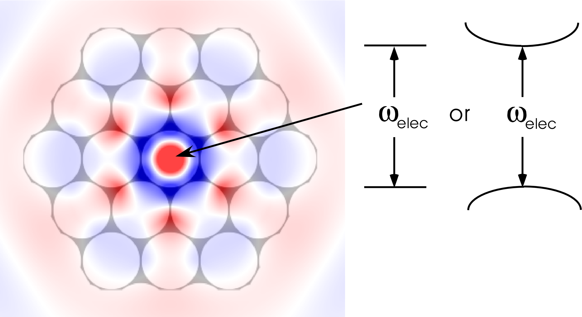
Figure 1: (Color) A 2D triangular lattice of air holes in dielectric ($\epsilon=13$). On top of the dielectric structure in grey, the $E_{z}$ field is plotted, with positive values in red, and negative values in blue. A small region of nonlinear material is placed exactly in the center of the structure. This material may be, for example, either two-level atoms, quantum wells, or some semiconductors such as InSb.

First, consider the magnitude of the enhancement or suppression of spontaneous emission in this system. Clearly, since there are several periods of high contrast dielectric, two effects are to be expected. First, there will be a substantial but incomplete suppression of emission inside the bandgap. Second, there will be an enhancement of spontaneous emission outside the bandgap (since the density of states is shifted to the frequencies surrounding the bandgap). For an atom polarized in the direction out of the 2-D plane, only the TM polarization need be considered.

We numerically obtain the enhancement of spontaneous emission by performing two time-domain simulations in Meep Farjadpour:06 , a finite difference time-domain code which solves Maxwell’s equations exactly with no approximations, apart from discretization (which can be systematically reduced) Taflove:00 . First, we calculate the spontaneous emission of a dipole placed in the middle of the photonic crystal structure illustrated in Fig. 1, then divide by the spontaneous emission rate observed in vacuum. The resulting values of $T_{1}$ and $T_{2}$ are calculated numerically, and Eq. (6), in conjunction with the definition of the enhancement factor $\eta$, is used to plot Fig. 3. The results are plotted in Fig. 2.

Figure 2: (Color) Relative enhancement of the TM local density of states for Fig. 1, as measured in the time-domain simulation rate of emission, $\Gamma$, normalized by the emission rate in vacuum, $\Gamma_{o}$

Figure 3: (Color) Contour plot of Kerr enhancement $\eta\equiv\mbox{Re}\,\chi^{(3)}_{\mbox{\tiny purcell}}/$ $\mbox{Re}\,\chi^{(3)}_{\mbox{\tiny hom}}$ as a function of probe ($\omega_{\mbox{\tiny ph}}$) and electronic transition ($\omega_{\mbox{\tiny elec}}$) frequencies, for a single quantum well of GaAs-AlGaAs, (a) at $T=200$ K, with $0.1\gamma_{\mbox{\tiny phase}}=10\Gamma_{\mbox{\tiny nr}}=\Gamma_{\mbox{\tiny rad}}$, and (b) at $T=225$ K, with $0.1\gamma_{\mbox{\tiny phase}}=\Gamma_{\mbox{\tiny nr}}=\Gamma_{\mbox{\tiny rad}}$.

A GaAs-AlGaAs single quantum well can lie in the interesting regime discussed above, where the radiative loss rate $\Gamma_{\mbox{\tiny rad}}$ dominates the non-radiative loss rate $\Gamma_{\mbox{\tiny nr}}$ as well as the overall loss rate of the quantum well, for certain temperatures Kraiem:01 . Equation (8) implies that one can see substantial enhancement of the Kerr coefficient in that regime.

At a temperature of about 200 K, $\Gamma_{\mbox{\tiny nr}}\approx 0.1\Gamma_{\mbox{\tiny rad}}$ Kraiem:01 . Although experimental measurements for $\gamma_{\mbox{\tiny phase}}$ are unavailable to the authors, the presence of a substantial phonon bath at that temperature leads one to expect a fairly large value, which may be conservatively estimated by $10\Gamma_{\mbox{\tiny rad}}$. These results are displayed in Fig. 3(a). Note that enhancement is primarily observed inside the photonic bandgap (cf. Fig. 2). We observe an enhancement in the real part of the Kerr coefficient up to a factor of 12, close to the predicted maximum enhancement factor of 10.48 in the regime of large detunings ($\Delta T_{2}\gg 1$).

Also, at a temperature of about 225 K, $\Gamma_{\mbox{\tiny nr}}\approx\Gamma_{\mbox{\tiny rad}}$ Kraiem:01 , and again we take $\gamma_{\mbox{\tiny phase}}=10\Gamma_{\mbox{\tiny rad}}$. These results are displayed in Fig. 3(b). In this case, we observe an enhancement up to a factor of 2.5, close to the predicted maximum enhancement factor of 1.91 in the regime of large detunings ($\Delta T_{2}\gg 1$).

Finally, we note that close to room temperature (285 K), the system in Ref. Kraiem:01, displays $\Gamma_{\mbox{\tiny nr}}\approx 10\Gamma_{\mbox{\tiny rad}}$, which is predicted to yield a maximum enhancement factor of 1.06. Since this number is fairly negligible, it illustrates that this approach has little impact when non-radiative losses dominate the decay of the electronic system.

On the other hand, some recent work has demonstrated that a single quantum dot can demonstrate predominantly radiative decay in vacuum even at room temperature, e.g., single CdSe/ZnS core-shell nanocrystals with a peak emission wavelength of 560 nm, with $\Gamma_{\mbox{\tiny rad}}\approx 39\Gamma_{\mbox{\tiny nr}}$ Brokmann:04 . Even bulk samples of similar nanocrystals have been shown to yield a significant radiative decay component, corresponding to $\Gamma_{\mbox{\tiny rad}}\approx\Gamma_{\mbox{\tiny nr}}$ Talapin:01 . Thus, we predict that with strong suppression of radiative decay, nonlinear enhancement of a factor of two, or more, could be observed at room temperature.

We now discuss the implications of this effect on previous work describing nonlinearities in photonic crystals, such as Ref. Soljacic:04, , and the references therein. Most past experiments should not have observed this effect, because they were designed with photonic bandgaps at optical frequencies significantly smaller than the frequencies of the electronic resonances generating the nonlinearities, in order to operate in a low-loss regime. Furthermore, in most materials, non-radiative decays will dominate radiative decays at room temperature. Finally, all the previous analyses are still valid as long as one considers the input parameters to be effective nonlinear susceptibilities, which come from natural nonlinear susceptibilities modified in the way described by this paper.

In conclusion, we have shown that the Purcell effect can be used to tailor optical nonlinearities. This principle manifests itself in an exemplary two-level system embedded in a photonic crystal; for realistic physical parameters, enhancement of Kerr nonlinearities by more than an order of magnitude is predicted. The described phenomena is caused by modifications of the local density of states near the resonant frequency. Thus, this treatment can easily be applied to analyze the Kerr nonlinearities of two-level systems in almost any geometrical structure in which the Purcell effect is substantial (e.g., photonic crystal fibers Litchinitser:02 , optical cavities). It also presents a reliable model for a variety of materials, such as quantum dots, atoms, and certain semiconductors. Future investigations will involve extending the formalism in this manuscript to other material systems.

The authors would like to thank Robert Boyd, Erich Ippen, Daniel Kleppner, Vladan Vuletic, Moti Segev, Steven G. Johnson, and Mark Rudner for valuable discussions. This work was supported in part by the Army Research Office through the Institute for Soldier Nanotechnologies under Contract No. DAAD-19-02-D0002. A.R. acknowledges the support of the Department of Energy under Grant No. DE-FG02-97ER25308.

References

- (1) P. Drazin and R. Johnson, Solitons: an Introduction (Cambridge University Press, Cambridge, England, 1989).
- (2) R. W. Boyd, Nonlinear Optics (Academic Press, San Diego, 1992).
- (3) M. Nielsen and I. Chuang, Quantum Computation and Quantum Information (Cambridge University Press, Cambridge, England, 2000).
- (4) G. Agrawal, Applications of Nonlinear Fiber Optics,, Optics and Photonics (Academic Press, San Diego, CA, 2001).
- (5) E. Purcell, Phys. Rev. 69, 681 (1946).
- (6) D. Kleppner, Phys. Rev. Lett. 47, 233 (1981).
- (7) H. Ryu and M. Notomi, Opt. Lett. 28, 2390 (2003).
- (8) P. Bermel, J. D. Joannopoulos, Y. Fink, P. A. Lane, and C. Tapalian, Phys. Rev. B 69, 035316 (2004).
- (9) D. Englund, D. Fattal, E. Waks, G. Solomon, B. Zhang, T. Nakaoka, Y. Arakawa, Y. Yamamoto, and J. Vuckovic, Phys. Rev. Lett. 95, 013904 (2005).
- (10) S. John and T. Quang, Phys. Rev. Lett. 76, 2484 (1996).
- (11) J. Preskill, Quantum Computation Lecture Notes, http://www.theory.caltech.edu/people/preskill/ph229/, 2004.
- (12) C. Cohen-Tannoudji, B. Diu, and F. Laloë, Quantum Mechanics (John Wiley and Sons, New York, 1977).
- (13) S. John and T. Quang, Phys. Rev. A 50, 1764 (1994).
- (14) P. Lambropoulos, G. M. Nikolopoulos, T. R. Nielsen, and S. Bay, Rep. Prog. Phys. 63, 455 (2000).
- (15) M. Bayer, T. L. Reinecke, F. Weidner, A. Larionov, A. McDonald, and A. Forchel, Phys. Rev. Lett. 86, 3168 (2001).
- (16) P. Lodahl, A. F. van Driel, I. S. Nikolaev, A. Irman, K. Overgaag, D. Vanmaekelbergh, and W. L. Vos, Nature 430, 654 (2004).
- (17) D. Miller, S. Smith, and B. Wherrett, Opt. Comm. 35, 221 (1980).
- (18) J. J. Sakurai, Modern Quantum Mechanics (Addison-Wesley, Reading, MA, 1994).
- (19) G. Lenz, J. Zimmermann, T. Katsufuji, M. E. Lines, H. Y. Hwang, S. Sp lter, R. E. Slusher, S.-W. Cheong, J. S. Sanghera, and I. D. Aggarwal, Opt. Lett. 25, 254 (2000).
- (20) A. Farjadpour, D. Roundy, A. Rodriguez, M. Ibanescu, P. Bermel, J. D. Joannopoulos, S. G. Johnson, and G. Burr, Opt. Lett. 31, 2972 (2006).
- (21) A. Taflove and S. C. Hagness, Computational Electrodynamics, 2nd ed. (Artech House, Norwood, MA, 2000).
- (22) S. Kraiem, F. Hassen, H. Maaref, X. Marie, and E. Vaneelle, Opt. Mat. 17, 305 (2001).
- (23) X. Brokmann, L. Coolen, M. Dahan, and J. P. Hermier, Phys. Rev. Lett. 93, 107403 (2004).
- (24) D. V. Talapin, A. L. Rogach, A. Kornowski, M. Haase, and H. Weller, Nano Lett. 1, 207 (2001).
- (25) M. Soljacic and J. D. Joannopoulos, Nature Mat. 3, 211 (2004).
- (26) N. M. Litchinitser, A. Abeeluck, C. Headley, and B. Eggleton, Opt. Lett. 27, 1592 (2002).