How Many Users should be Turned On
in a Multi-Antenna Broadcast Channel?^∗

Abstract

This paper considers broadcast channels with $L$ antennas at the base station and $m$ single-antenna users, where each user has perfect channel knowledge and the base station obtains channel information through a finite rate feedback. The key observation of this paper is that the optimal number of on-users (users turned on), say $s$, is a function of signal-to-noise ratio (SNR) and other system parameters. Towards this observation, we use asymptotic analysis to guide the design of feedback and transmission strategies. As $L$, $m$ and the feedback rates approach infinity linearly, we derive the asymptotic optimal feedback strategy and a realistic criterion to decide which users should be turned on. Define the corresponding asymptotic throughput per antenna as the spatial efficiency. It is a function of the number of on-users $s$, and therefore, $s$ should be appropriately chosen. Based on the above asymptotic results, we also develop a scheme for a system with finite many antennas and users. Compared with other works where $s$ is presumed constant, our scheme achieves a significant gain by choosing the appropriate $s$. Furthermore, our analysis and scheme is valid for heterogeneous systems where different users may have different path loss coefficients and feedback rates.

I Introduction

It is well known that multiple antennas can improve the spectral efficiency. This paper considers broadcast channels with $L$ antennas at the base station and $m$ single-antenna users. To achieve the full benefit, perfect channel state information (CSI) is required at both receiver and transmitter. Perfect CSI at the receiver can be obtained by estimation from the received signal. However, if CSI at the transmitter (CSIT) is obtained from feedback, perfect CSIT requires an infinite feedback rate. As this is not feasible in practice, it is important to analyze the effect of finite rate feedback and design efficient strategy accordingly.

The feedback models for broadcast channels are described as follows. To save feedback rate on power control, we assume a power on/off strategy where each user is either turned on with a constant power or turned off, and that the number of on-users (the users turned on) is a constant, say $s$, independent of the channel realization. For any given channel realization, the users quantize their channel states into finite bits and feedback the corresponding indices to the base station. After receiving the feedback from users, the base station decides which users should be turned on and then forms beamforming vectors for transmission.

Broadcast channels with feedback have been studied in [1, 2]. Ideally, if the base station has the perfect CSI, zero-forcing transmission avoids interference among users. However, with only finite rate feedback on CSI, the base station does not know the perfect channel state information and therefore interference from other users is inevitable. The interference gets so strong at high signal-to-noise ratio (SNR) regions that the system throughput is upper bounded by a constant even when SNR approach infinity. This phenomenon is called interference domination and was reported on in [1, 2]. The analysis is based on the assumption that the number of on-users $s$ always equals to the number of antennas at the base station $L$ ($L\leq m$ is typically assumed). To limit the interference to a desired level, Sharif and Hassibi let $m$ grow exponentially with $L$ such that there are $L$ near orthogonal users with high probability [1]. In both scenarios, a homogeneous system is assumed where all the users share the same path loss coefficient and feedback resource.

Different from the above approaches, this paper studies heterogeneous broadcast systems, where different users may have different path loss coefficients and feedback rates. Furthermore, different from [1], we focus on systems with a relatively small number of users. Note that a cooperative communication network can often be viewed as a composition of multi-access and broadcast sub-systems with a small number of users. Research on broadcast systems of small size provides insights into cooperative communications.

For such systems, we solve the interference domination problem by choosing the appropriate number of on-users $s$. The reason that random beams construction in [1] fails in our small size systems is elaborated in Theorem 2.

Our solution is based on the asymptotic analysis where $L,m,s$ and the feedback rates approach infinity linearly with constant ratios among them. This type of asymptotics is applied to systems of small size. The main asymptotic results are:

• It is asymptotically optimal to quantize the channel directions only and ignore the channel magnitude information. The asymptotically optimal feedback function and codebook are derived accordingly.

• A realistic on/off criterion is proposed to decide which users should be turned on.

• The corresponding throughput per antenna converges to a constant, defined as the spatial efficiency. It is a function of the normalized number of on-users $\bar{s}=\frac{s}{L}$. Further, there exists a unique $\bar{s}\in\left(0,1\right)$ to maximize the the spatial efficiency.

We develop a scheme to choose the appropriate $s$ for systems with finite $L$ and $m$. Simulations show that the gain achieved by choosing $s$ is significant compared with the strategies where $s\equiv L$. In addition, our scheme has the following advantages.

• It is valid for heterogeneous systems.

• The set of on-users is independent of the channel realization. As a result, computation complexity is low since we do not have to perform a user selection computation every fading block.

• Only on-users need to feedback CSI, which saves a large amount of feedback resource.

This paper is organized as follows. The system model is introduced in Section II. Then Section III performs the asymptotic analysis obtaining insights into system design, and quantifies the spatial efficiency. Based on the asymptotic results, a practical scheme is developed in Section IV for systems with finite many antennas and users. Finally, conclusions are summarized in Section V.

II System Model

Consider a broadcast channel with $L$ antennas at the base station and $m$ single-antenna users. Assume that the base station employs zero forcing transmitter. Let $\gamma_{i}\in\mathbb{R}\backslash\mathbb{R}^{-}$ ($1\leq i\leq m$) be the path loss coefficient for user $i$. Then the signal model for user $i$ is

$$Y_{i}=\sqrt{\gamma_{i}}\mathbf{h}_{i}^{\dagger}\left(\sum_{j=1}^{m}\mathbf{q}_{j}X_{j}\right)+W_{i},$$

where $Y_{i}\in\mathbb{C}$ is the received signal for user $i$, $\mathbf{h}_{i}\in\mathbb{C}^{L\times 1}$ is the channel state vector for user, $\mathbf{q}_{j}\in\mathbb{C}^{L\times 1}$ is the zero-forcing beamforming vector for user $j$, $X_{j}\in\mathbb{C}$ is the source signal for the user $j$ and $W_{i}\in\mathbb{C}$ is the complex Gaussian noise with zero mean and unit variance $\mathcal{CN}\left(0,1\right)$. Here, we assume that $\mathbf{q}_{j}^{\dagger}\mathbf{q}_{j}=1$ and the Rayleigh block fading channel model: the entries of $\mathbf{h}_{i}$ are independent and identically distributed (i.i.d.) $\mathcal{CN}\left(0,1\right)$. Without loss of generality, we assume that $L\leq m$; if $L>m$, adding $L-m$ users with $\gamma_{i}=0$ yields an equivalent system with $L^{\prime}=m$.

For the above broadcast system, it is natural to assume a total power constraint $\sum_{i=1}^{m}\mathrm{E}\left[\left|X_{i}\right|^{2}\right]\leq\rho$. Further, for implementation simplicity, we assume a power on/off strategy with a constant number of on-users as follows.

A1)

Power on/off strategy: a source $X_{i}$ is either turned on with a constant power $P_{\mathrm{on}}$ or turned off. It is motivated by the fact that this strategy is near optimal for single user MIMO system [3].

A2)

A constant number of on-users: we assume that the number of on-users $s$ ($1\leq s\leq m$) is a constant independent of the specific channel realizations. With this assumption, $P_{\mathrm{on}}=\frac{\rho}{s}$. Here, $s$ is a function of $\rho$, $\gamma_{i}$ and feedback rate. This assumption is different from the one in [1, 2], where $s=L$ always ($L\leq m$ is assumed there).

The finite rate feedback model is then described as follows. Assume that both base station and user $i$ knows $\gamma_{i}$ but only user $i$ knows the channel state realization $\mathbf{h}_{i}$ perfectly. For given channel realizations $\mathbf{h}_{1}\cdots\mathbf{h}_{m}$, user $i$ quantizes his channel $\mathbf{h}_{i}$ into $R_{i}$ bits and then feeds the corresponding index to the base station. Formally, let $\mathcal{B}_{i}=\left\{\hat{\mathbf{h}}\in\mathbb{C}^{L\times 1}\right\}$ with $\left|\mathcal{B}_{i}\right|=2^{R_{i}}$ be a channel state codebook for user $i$. Then the quantization function is given by

$$\mathfrak{q}:\mathbb{C}^{L\times 1} \rightarrow\mathcal{B}_{i}$$

$$\mathbf{h}_{i} \mapsto\hat{\mathbf{h}}_{i}.$$

In Section III-A and III-B, we will show how to design $\mathfrak{q}$ and $\mathcal{B}$ respectively.

After receiving feedback information from users, the base station decides which $s$ users should be turned on and forms zero-forcing beamforming vectors for them. Let $A_{\mathrm{on}}$ be the set of $s$ on-users. The zero-forcing beamforming vectors $\mathbf{q}_{i}$’s $i\in A_{\mathrm{on}}$ is calculated as follows. Let $\mathcal{P}_{i}^{\perp}$ be the plane generated by $\left\{\hat{\mathbf{h}}_{j}:\;j\in A_{\mathrm{on}}\backslash\left\{i\right\}\right\}$. Let $\mathcal{P}_{i}$ be the orthogonal complement of $\mathcal{P}_{i}^{\perp}$ and $t$ be the dimensions of $\mathcal{P}_{i}$. Define $\mathbf{T}_{i}\in\mathbb{C}^{L\times t}$ the matrix whose columns are orthonormal and span the plane $\mathcal{P}$. Then $\mathbf{q}_{i}$ is the unitary projection of $\hat{\mathbf{h}}_{i}$on $\mathbf{T}_{i}$

$$\mathbf{q}_{i}:=\frac{\mathbf{T}_{i}\mathbf{T}_{i}^{\dagger}\hat{\mathbf{h}}_{i}}{\left\|\mathbf{T}_{i}\mathbf{T}_{i}^{\dagger}\hat{\mathbf{h}}_{i}\right\|}.$$ (1)

Here, if $s=1$ and $A_{\mathrm{on}}=\left\{i\right\}$, $\mathbf{T}_{i}$ is a $L\times L$ unitary matrix and $\mathbf{q}_{i}=\hat{\mathbf{h}}_{i}/\left\|\hat{\mathbf{h}}_{i}\right\|$.

III Asymptotic Analysis

In order to obtain insights into system design, this section performs asymptotic analysis by letting $L,m,R_{i}\mathrm{{}^{\prime}s}\rightarrow\infty$ linearly. The quantization function $\mathfrak{q}$ and asymptotically optimal codebook $\mathcal{B}_{i}$ are derived in Section III-A and III-B respectively. Then Section III-C develops a realistic on/off criterion to decide which users should be turned on. Finally Section III-D computes the corresponding spatial efficiency.

III-A Design of Quantization Function

Generally speaking, full information of $\mathbf{h}_{i}$ contains the direction information $\mathbf{v}_{i}:=\mathbf{h}_{i}/\left\|\mathbf{h}_{i}\right\|$ and the magnitude information $\left\|\mathbf{h}_{i}\right\|$. In our Rayleigh fading channel model, it is well known that $\mathbf{v}_{i}$ and $\left\|\mathbf{h}_{i}\right\|$ are independent. Intuitively, joint quantization of $\mathbf{v}_{i}$ and $\left\|\mathbf{h}_{i}\right\|$ is preferred.

Interestingly, Theorem 1 implies that there is no need to quantize the channel magnitudes. Indeed, as $L,m\rightarrow\infty$ linearly, all users’ channel magnitudes concentrate on a single value with probability one.

Theorem 1

For $\forall\epsilon>0$, as $L,m\rightarrow\infty$ with $\frac{m}{L}\rightarrow\bar{m}\in\mathbb{R}^{+}$,

$$\Pr\left(\underset{1\leq i\leq m}{\max}\;\frac{1}{L}\left\|\mathbf{h}_{i}\right\|^{2}\geq 1+\epsilon\right)\rightarrow 0,$$

and

$$\Pr\left(\underset{1\leq i\leq m}{\min}\;\frac{1}{L}\left\|\mathbf{h}_{i}\right\|^{2}\leq 1-\epsilon\right)\rightarrow 0.$$

The proof of Theorem 1 is omitted due to the space limitation. An important fact behind the proof is that whether the users’ channel magnitudes concentrate or not depends on the relationship between $L$ and $m$: this concentration happens in our asymptotic region where $L$ and $m$ are of the same order.

To fully understand Theorem 1, it is important to realize that the Law of Large Numbers does not imply that all users’ channel magnitudes will concentrate. According to the Law of Large Numbers, $\frac{1}{L}\left\|\mathbf{h}_{i}\right\|\rightarrow 1$ almost surely for any given $i$. However, if $m$ approaches infinity exponentially with $L$, there are certain number of users whose channel magnitudes are larger than others’, and therefore it may be still beneficial to quantize and feedback channel magnitude information. This phenomenon is illustrated by the following example.

Example 1

(A case where magnitude information is beneficial) Consider a broadcast channel with $\gamma_{1}=\cdots=\gamma_{m}=1$. As $L,m\rightarrow\infty$ with $\log\left(m\right)/L\rightarrow\bar{m}^{\prime}\in\mathbb{R}^{+}$, there exists an $\epsilon>0,$ $\delta_{1}>0$ and $\delta_{2}>0$ such that

$$\frac{1}{L}\log\left|\left\{i:\;\frac{1}{L}\left\|\mathbf{h}_{i}\right\|^{2}>1+\frac{\epsilon}{2}\right\}\right|\rightarrow\delta_{1},$$

and

$$\frac{1}{L}\log\left|\left\{i:\;\frac{1}{L}\left\|\mathbf{h}_{i}\right\|^{2}<1-\frac{\epsilon}{2}\right\}\right|\rightarrow\delta_{2}$$

with probability one. Note that there are a set of users whose channel magnitudes are $\epsilon$-larger than another set of users. It may be worth to let the base station know which users have stronger channels.

Theorem 1 implies that it is sufficient to quantize the channel direction information only and omit the channel magnitude information. For this quantization, the codebook is given by $\mathcal{B}_{i}=\left\{\mathbf{p}\in\mathbb{C}^{L\times 1}:\;\left\|\mathbf{p}\right\|=1\right\}$ with $\left|\mathcal{B}_{i}\right|=2^{R_{i}}$. We use the following quantization function

$$\mathfrak{q}:\mathbb{C}^{L\times 1} \rightarrow\mathcal{B}_{i}$$

$$\mathbf{h}_{i} \mapsto\mathbf{p}_{i}=\underset{\mathbf{p}\in\mathcal{B}_{i}}{\arg\;\max}\;\left|\mathbf{v}_{i}^{\dagger}\mathbf{p}\right|,$$ (2)

where $\mathbf{v}_{i}$ is the channel direction vector.

III-B Asymptotically Optimal Codebooks

Given the quantization function (2), the distortion of a given codebook $\mathcal{B}_{i}$ is the average chordal distance between the actual and quantized channel directions corresponding to the codebook $\mathcal{B}_{i}$ and defined as

$$D\left(\mathcal{B}_{i}\right):=1-\mathrm{E}_{\mathbf{h}_{i}}\left[\underset{\mathbf{p}\in\mathcal{B}_{i}}{\max}\left|\mathbf{v}_{i}^{\dagger}\mathbf{p}\right|^{2}\right].$$

The following lemma bounds the minimum achievable distortion for a given codebook rate (usually called the distortion rate function).

Lemma 1

Define $D^{*}\left(R\right)\triangleq\underset{\mathcal{B}:\;\left|\mathcal{B}\right|\leq 2^{R}}{\inf}D\left(\mathcal{B}\right)$. Then

$$\frac{L-1}{L}2^{-\frac{R}{L-1}}\left(1+o\left(1\right)\right)\leq D^{*}\left(R\right)$$

$$\quad\quad\quad\leq\frac{\Gamma\left(\frac{1}{L-1}\right)}{L-1}2^{-\frac{R}{L-1}}\left(1+o\left(1\right)\right),$$ (3)

and as $L$ and $R$ approach infinity with $\frac{R}{L}\rightarrow\bar{r}\in\mathbb{R}^{+}$,

$$\underset{\left(L,R\right)\rightarrow\infty}{\lim}D^{*}\left(R\right)=2^{-\bar{r}}.$$

The following Lemma shows that a random codebook is asymptotically optimal with probability one.

Lemma 2

Let $\mathcal{B}_{\mathrm{rand}}$ be a random codebook where the vectors $\mathbf{p}\in\mathcal{B}_{\mathrm{rand}}$’s are independently generated from the isotropic distribution. Let $R=\log\left|\mathcal{B}_{\mathrm{rand}}\right|$. As $L,R\rightarrow\infty$ with $\frac{R}{L}\rightarrow\bar{r}\in\mathbb{R}^{+}$, for $\forall\epsilon>0$,

$$\underset{\left(L,R\right)\rightarrow\infty}{\lim}\;\mathrm{Pr}\left\{\mathcal{B}_{\mathrm{rand}}:\;D\left(\mathcal{B}_{\mathrm{rand}}\right)>2^{-\bar{r}}+\epsilon\right\}=0.$$

The proofs of Lemma 1 and 2 are given in our paper [4].

Due to the asymptotic optimality of random codebooks, we assume that the codebooks $\mathcal{B}_{i}$’s $i=1,\cdots,m$ are independent and randomly constructed throughout this paper.

III-C On/off Criterion

After receiving feedback from users, the base station should decide which $s$ users should be turned on.

Ideally, for given channel realizations $\mathbf{h}_{1},\cdots,\mathbf{h}_{m}$, the optimal set of on users $A_{\mathrm{on}}^{*}$ should be chosen to maximize the instantaneous mutual information. Note that the base station only knows the quantized version of channel states $\mathbf{p}_{1},\cdots,\mathbf{p}_{m}$. It can only estimate the instantaneous mutual information through $\mathbf{p}_{i}$’s. The set $A_{\mathrm{on}}^{*}$ is given by

$$A_{\mathrm{on}}^{*}= \underset{A_{\mathrm{on}}:\;\left|A_{\mathrm{on}}\right|=s}{\arg\;\max}\;\sum_{i\in A_{\mathrm{on}}}\log\left(1+\right.$$

$$\quad\quad\quad\left.\frac{\gamma_{i}\frac{\rho}{s}\left|\mathbf{p}_{i}^{\dagger}\mathbf{q}_{i}\right|^{2}}{1+\gamma_{i}\frac{\rho}{s}\sum_{j\in A_{\mathrm{on}}\backslash\left\{i\right\}}\left|\mathbf{p}_{i}^{\dagger}\mathbf{q}_{j}\right|^{2}}\right).$$ (4)

However, finding $A_{\mathrm{on}}^{*}$ requires exhaustive search, whose complexity exponentially increases with $m$.

The random orthonormal beams construction method in [1] does not work for our asymptotically large system either. In [1], the base station randomly constructs $L$ orthonormal beams $\mathbf{b}_{1},\cdots,\mathbf{b}_{L}$, finds the users with highest signal-to-noise-plus-interference ratios (SINRs) through feedback from users, and then transmits to these selected users. There, the SINR calculation for user $i$ is related to the quantity $\underset{1\leq k\leq L}{\max}\left|\mathbf{h}_{i}^{\dagger}\mathbf{b}_{k}\right|$. However, Theorem 2 below shows that in the asymptotic region where $L$ and $m$ are of the same order, all users’ channels are near orthogonal to all of the $L$ orthonormal beams $\mathbf{b}_{i}$’s. Therefore, all users’ maximum SINRs (maximum over $L$ given orthonormal beams) approach zero uniformly with probability one. The method in [1] fails in our asymptotically large system.

Theorem 2

Given $\forall\epsilon>0$ and any $L$ orthonormal beams $\mathbf{b}_{k}\in\mathbb{C}^{L\times 1}$ $1\leq k\leq L$, as $L,m\rightarrow\infty$ linearly with $\frac{m}{L}\rightarrow\bar{m}\in\mathbb{R}^{+}$,

$$\underset{\left(L,m\right)\rightarrow\infty}{\lim}\;\Pr\left(\underset{1\leq i\leq m,\;1\leq k\leq L}{\max}\;\frac{1}{L}\left|\mathbf{h}_{i}^{\dagger}\mathbf{b}_{k}\right|>\epsilon\right)=0.$$

The proof is omitted due to the space limitation.

In this paper, we take another approach where the on/off decision is independent of channel directions. We start with the throughput analysis for a specific on-user $i\in A_{\mathrm{on}}$. Note that

$$Y_{i}=\sqrt{\gamma_{i}}\mathbf{h}_{i}^{\dagger}\mathbf{q}_{i}X_{i}+\left(\sqrt{\gamma_{i}}\mathbf{h}_{i}^{\dagger}\sum_{j\in A_{\mathrm{on}}\backslash\left\{i\right\}}\mathbf{q}_{j}X_{j}+W\right).$$

The signal power and interference power for user $i$ are given by

$$P_{\mathrm{sig},i}=\frac{\rho}{s}\gamma_{i}\left|\mathbf{h}_{i}^{\dagger}\mathbf{q}_{i}\right|^{2}$$ (5)

and

$$P_{\mathrm{int},i}=\frac{\rho}{s}\gamma_{i}\sum_{j\in A_{\mathrm{on}}\backslash\left\{i\right\}}\left|\mathbf{h}_{i}^{\dagger}\mathbf{q}_{j}\right|^{2}$$ (6)

respectively. Note that the influence of the users in $A_{\mathrm{on}}\backslash\left\{i\right\}$ on user $i$ only occurs through their directions $\mathbf{q}_{j}$’s $j\in A_{\mathrm{on}}\backslash\left\{i\right\}$. If the choice of on-users $A_{\mathrm{on}}$ is independent of their channel directions, then $\mathbf{h}_{i}$ and $\mathbf{q}_{j}$’s are independent. In this case, $P_{\mathrm{sig},i}$ and $P_{\mathrm{int},i}$ can be quantified as $L,m,s,R_{i}\mathrm{{}^{\prime}s}\rightarrow\infty$. The result is given in the following proposition.

Proposition 1

Let $\left|A_{\mathrm{on}}\right|=s$ and $L,m,s,R_{i}\mathrm{{}^{\prime}s}\rightarrow\infty$ with $\frac{m}{L}\rightarrow\bar{m}$, $\frac{s}{L}\rightarrow\bar{s}$ and $\frac{R_{i}}{L}\rightarrow\bar{r}_{i}$. Assume that $\mathbf{v}_{i}$’s $i\in A_{\mathrm{on}}$ are independent. Then for $\forall i\in A_{\mathrm{on}}$,

$$P_{\mathrm{sig},i}\rightarrow\frac{\rho}{\bar{s}}\gamma_{i}\left(1-2^{-\bar{r}_{i}}\right)\left(1-\bar{s}\right),$$

$$P_{\mathrm{int},i}\rightarrow\rho\gamma_{i}2^{-\bar{r}_{i}},$$

and therefore

$$\mathcal{I}_{i} :=\log\left(1+\frac{P_{\mathrm{sig},i}}{1+P_{\mathrm{int},i}}\right)$$

$$\rightarrow\log\left(1+\eta_{i}\frac{1-\bar{s}}{\bar{s}}\right),$$

with probability one, where

$$\eta_{i}:=\frac{\rho\gamma_{i}\left(1-2^{-\bar{r}_{i}}\right)}{1+\rho\gamma_{i}2^{-\bar{r}_{i}}}.$$ (7)

Remark 1

This proposition may not be true if $\mathbf{v}_{j}$’s ($j\in A_{\mathrm{on}}\backslash\left\{i\right\}$) are not independent of $\mathbf{v}_{i}$. Indeed, for example, if other users are chosen such that their channel directions are as orthogonal to user $i$ as possible, the interference to user $i$ is less than that achieved by our choice where channel directions are not taken into consideration. This claim is verified by the fact that $\exists\epsilon>0$ such that

$$\underset{A_{\mathrm{on}}\backslash\left\{i\right\}}{\min}\;\sum_{j\in A_{\mathrm{on}}\backslash\left\{i\right\}}\left|\mathbf{h}_{i}^{\dagger}\mathbf{q}_{j}\right|^{2}<\sum_{j\in A_{\mathrm{on},\mathrm{rand}}\backslash\left\{i\right\}}\left|\mathbf{h}_{i}^{\dagger}\mathbf{q}_{j}\right|^{2}-\epsilon$$

with probability one as $L,m,s\rightarrow\infty$ linearly, where $A_{\mathrm{on,}\mathrm{rand}}\backslash\left\{i\right\}$ denotes a random choice of $A_{\mathrm{on}}\backslash\left\{i\right\}$.

Remark 2

Proposition 1 shows that the user $i$’s asymptotic throughput is a constant independent of the specific channel realization $\mathbf{h}_{i}$ with probability one.

Based on Proposition 1, we select the set of $s$ on-users $A_{\mathrm{on}}$ such that $\left|A_{\mathrm{on}}\right|=s$ and

$$A_{\mathrm{on}}=\left\{i:\;\eta_{i}\geq\eta_{j}\;\mathrm{for}\;\forall j\notin A_{\mathrm{on}}\right\};$$ (8)

if there are multiple candidates, we randomly choose one of them. It is the asymptotically optimal on/off selection if the on/off decision is independent of the channel direction information. The difference between the throughput achieved by optimal on/off criterion in (8) and the proposed one in (4) remains unknown.

III-D The Spatial Efficiency

We define the spatial efficiency (bits/sec/Hz/antenna) as

$$\bar{\mathcal{I}}\left(\bar{s}\right):=\underset{\left(L,m,s,R_{i}\mathrm{{}^{\prime}s}\right)\rightarrow\infty}{\lim}\bar{\mathcal{I}}^{\left(L\right)},$$

where $L,m,s,R_{i}\mathrm{{}^{\prime}s}\rightarrow\infty$ in the same way as before, $\bar{\mathcal{I}}^{\left(L\right)}$ is the average throughput per antenna given by

$$\bar{\mathcal{I}}^{\left(L\right)}:=\mathrm{E}_{\mathcal{B}_{i}\mathrm{{}^{\prime}s},\mathbf{h}_{i}\mathrm{{}^{\prime}s}}\left[\frac{1}{L}\sum_{i\in A_{\mathrm{on}}}\log\left(1+\frac{P_{\mathrm{sig},i}}{1+P_{\mathrm{int},i}}\right)\right],$$

and $A_{\mathrm{on}}$, $P_{\mathrm{sig},i}$ and $P_{\mathrm{int},i}$ are defined in (8), (5) and (6) respectively.

We shall quantify $\bar{\mathcal{I}}\left(\bar{s}\right)$ for a given $\bar{s}$. Define the empirical distribution of $\eta_{i}$ as

$$\mu_{\eta}^{\left(m\right)}\left(\eta\leq x\right):=\frac{1}{m}\left|\left\{\eta_{i}:\;\eta_{i}\leq x\right\}\right|,$$

and assume that $\mu_{\eta}:=\lim\mu_{\eta}^{\left(m\right)}$ exists weakly as $L,m,R_{i}\mathrm{{}^{\prime}s}\rightarrow\infty$. In order to cope with $\mu_{\eta}$’s with mass points, define

$$\int_{x^{+}}^{\infty}f\left(\eta\right)d\mu_{\eta}:=\underset{\Delta x\downarrow 0}{\lim}\int_{x+\Delta x}^{\infty}f\left(\eta\right)d\mu_{\eta}$$

for $\forall x\in\mathbb{R}$, where $f$ is a integrable function with respect to $\mu_{\eta}$. Then $\bar{\mathcal{I}}\left(\bar{s}\right)$ is computed in the following theorem.

Theorem 3

Let $L,m,s,R_{i}\mathrm{{}^{\prime}s}\rightarrow\infty$ with $\frac{m}{L}\rightarrow\bar{m}$, $\frac{s}{L}\rightarrow\bar{s}$ and $\frac{R_{i}}{L}\rightarrow\bar{r}_{i}$. Define

$$\eta_{\bar{s}}:=\sup\left\{\eta:\;\bar{m}\int_{\eta}^{\infty}d\mu_{\eta}>\bar{s}\right\}.$$

Then as $\bar{s}\notin\left(0,1\right)$, $\bar{\mathcal{I}}\left(\bar{s}\right)=0$. If $\bar{s}\in\left(0,1\right)$,

$$\bar{\mathcal{I}}\left(\bar{s}\right) =\bar{m}\int_{\eta_{\bar{s}}^{+}}^{\infty}\log\left(1+\eta\frac{1-\bar{s}}{\bar{s}}\right)d\mu_{\eta}$$

$$\quad+\left(\bar{s}-\bar{m}\int_{\eta_{\bar{s}}^{+}}^{\infty}d\mu_{\eta}\right)\log\left(1+\eta_{\bar{s}}\frac{1-\bar{s}}{\bar{s}}\right).$$ (9)

We are also interested in finding the optimal $\bar{s}$ to maximize $\bar{\mathcal{I}}\left(\bar{s}\right)$. Unfortunately, $\bar{\mathcal{I}}\left(\bar{s}\right)$ is not a concave function of $\bar{s}$ in general. Furthermore, the measure $\mu_{\eta}$ may contain mass points. The optimization of $\bar{\mathcal{I}}\left(\bar{s}\right)$ is therefore a non-convex and non-smooth optimization problem. The following theorem provides a criterion to find the optimal $\bar{\mathcal{I}}\left(\bar{s}\right)$.

Theorem 4

$\bar{\mathcal{I}}\left(\bar{s}\right)$ is maximized at a unique $\bar{s}^{*}\in\left(0,1\right)$ such that

$$0\in\left[\underset{\Delta\bar{s}\rightarrow 0}{\lim\;\inf}\frac{\bar{\mathcal{I}}\left(\bar{s}^{*}\right)-\bar{\mathcal{I}}\left(\bar{s}^{*}-\Delta\bar{s}\right)}{\Delta\bar{s}},\right.$$

$$\quad\quad\left.\underset{\Delta\bar{s}\rightarrow 0}{\lim\;\sup}\frac{\bar{\mathcal{I}}\left(\bar{s}^{*}\right)-\bar{\mathcal{I}}\left(\bar{s}^{*}-\Delta\bar{s}\right)}{\Delta\bar{s}}\right].$$ (10)

The proof is omitted due to the space limitation. The $\bar{\mathcal{I}}\left(\bar{s}^{*}\right)$ is the maximum achievable spatial efficiency for the proposed power on/off strategy.

IV Finite Dimensional System Design

Based on the asymptotic results in Theorem 3-4, we now propose a scheme for systems with finite $L$ and $m$.

IV-A Throughput Estimation for Finite Dimensional Systems

While asymptotic analysis provide many insights, we do not apply asymptotic results directly for a finite dimensional system. The reason is that in asymptotic analysis $\frac{1}{L}\rightarrow 0$ while $\frac{1}{L}$ cannot be ignored for a system with small $L$. In the following, we first calculate the main order term of the throughput for user $i\in A_{\mathrm{on}}$ and then explain the difference between asymptotic analysis and finite dimensional system analysis explicitly.

To obtain the main order term, proceed as follows. Note that the throughput for user $i\in A_{\mathrm{on}}$ ($\left|A_{\mathrm{on}}\right|=s$) is

$$\mathcal{I}_{i} =\mathrm{E}\left[\log\left(1+\frac{P_{\mathrm{sig},i}}{1+P_{\mathrm{int},i}}\right)\right]$$

$$=\log\left(1+\frac{\mathrm{E}\left[P_{\mathrm{sig},i}\right]}{1+\mathrm{E}\left[P_{\mathrm{int},i}\right]}\right)$$

$$\quad+\mathrm{E}\left[\log\left(\frac{1+P_{\mathrm{sig},i}+P_{\mathrm{int},i}}{1+\mathrm{E}\left[P_{\mathrm{sig},i}\right]+\mathrm{E}\left[P_{\mathrm{int},i}\right]}\right)\right]$$

$$\quad-\mathrm{E}\left[\log\left(\frac{1+P_{\mathrm{int},i}}{1+\mathrm{E}\left[P_{\mathrm{int},i}\right]}\right)\right],$$

where $P_{\mathrm{sig},i}$ and $P_{\mathrm{int},i}$ are defined in (5) and (6). The following theorem calculates $\mathrm{E}\left[P_{\mathrm{sig},i}\right]$ and $\mathrm{E}\left[P_{\mathrm{int},i}\right]$ for finite dimensional systems.

Theorem 5

Let $\mathcal{B}_{i}$’s be randomly constructed and $D_{i}=\mathrm{E}_{\mathcal{B}_{i}}\left[D\left(\mathcal{B}_{i}\right)\right]$ for all $1\leq i\leq m$. For randomly chosen $A_{\mathrm{on}}$ and $i\in A_{\mathrm{on}}$, if $1\leq s\leq L$

$$\mathrm{E}\left[P_{\mathrm{sig},i}\right]=\gamma_{i}\rho\frac{L}{s}\left[\left(1-D_{i}\right)\left(1-\frac{s-1}{L}\right)+D_{i}\frac{s-1}{L\left(L-1\right)}\right],$$ (11)

and

$$\mathrm{E}\left[P_{\mathrm{int},i}\right]=\gamma_{i}\rho\frac{L}{s}\frac{s-1}{L-1}D_{i};$$ (12)

if $s>L$, $\mathrm{E}\left[P_{\mathrm{sig},i}\right]=0$.

The calculation of $\mathrm{E}\left[P_{\mathrm{sig},i}\right]$ and $\mathrm{E}\left[P_{\mathrm{int},i}\right]$ relies on quantification of $D_{i}$. In general, it is difficult to compute $D_{i}$ precisely. Note that the upper bound in (3) is derived by evaluating the average performance of random codebooks (see [4] for details). We use its main order term to estimate $D_{i}$:

$$D_{i}\approx\frac{\Gamma\left(\frac{1}{L-1}\right)}{L-1}2^{-\frac{R_{i}}{L-1}}.$$

Define

$$\mathcal{I}_{\mathrm{main},i}:=\log\left(1+\frac{\mathrm{E}\left[P_{\mathrm{sig},i}\right]}{1+\mathrm{E}\left[P_{\mathrm{int},i}\right]}\right).$$ (13)

It can be verified from Proposition 1 that $\mathcal{I}_{i}=\mathcal{I}_{\mathrm{main},i}+o\left(1\right)$ and therefore $\mathcal{I}_{\mathrm{main},i}$ is the main order term of $\mathcal{I}_{i}$.

Then the difference between asymptotic analysis and finite dimensional systems analysis is clear. In the limit, $\frac{s-1}{L}\rightarrow\bar{s}$ and $\frac{R_{i}}{L-1}\rightarrow\bar{r}_{i}$. However, for finite dimensional systems, simply substituting these asymptotic values into (11-13) directly introduces unpleasant error, especially when $L$ is small. Therefore, to estimate $\mathcal{I}_{i}$ ($\forall i\in A_{\mathrm{on}}$) for finite dimensional systems, we have to rely on (11-13).

IV-B A Scheme for Finite Dimensional Systems

Given system parameters $L$, $m$, $\gamma_{i}$’s and $R_{i}$’s, a practical scheme needs to calculate the appropriate $s$ and $A_{\mathrm{on}}$. This process is described in the following.

For a given $s$, the set of $A_{\mathrm{on}}$ is decided as follows: we first calculate $\mathcal{I}_{\mathrm{main},1},\cdots,\mathcal{I}_{\mathrm{main},m}$ according to (13) and then choose the $s$ users with the largest $\mathcal{I}_{\mathrm{main},i}$’s to turn on; if there exists any ambiguity, random selection is employed to resolve it. For example, if $\mathcal{I}_{\mathrm{main},1}>\mathcal{I}_{\mathrm{main},2}>\cdots>\mathcal{I}_{\mathrm{main},m}$, the user $1,2,\cdots,s$ are turned on. If $\mathcal{I}_{\mathrm{main},1}=\mathcal{I}_{\mathrm{main},2}=\cdots=\mathcal{I}_{\mathrm{main},m}$, the $s$ on-users are randomly selected from all the $m$ users. Note again, $A_{\mathrm{on}}$ is independent of the channel realization.

The appropriate $s$ is chosen as follows. Let

$$\mathcal{I}_{\mathrm{main}}\left(s\right)=\underset{A_{\mathrm{on}}:\;\left|A_{\mathrm{on}}\right|=s}{\max}\;\sum_{i\in A_{\mathrm{on}}}\mathcal{I}_{\mathrm{main},i}.$$

Here, note that $\mathcal{I}_{\mathrm{main},i}$ is a function of $s$. For a given broadcast system, we choose the number of on-users to be

$$s_{\mathrm{main}}^{*}=\underset{1\leq s\leq L}{\arg\;\max}\;\mathcal{I}_{\mathrm{main}}\left(s\right).$$

Although the above procedure involves exhaustive search, the corresponding complexity is actually low. First, the calculations are independent of instantaneous channel realizations. Only system parameters $L$, $m$, $\gamma_{i}$’s and $R_{i}$’s are needed. Provided that $\gamma_{i}$’s change slowly, the base station does not need to recalculate $s_{\mathrm{main}}^{*}$ and $A_{\mathrm{on}}$ frequently. Second, $R_{i}=R_{j}$ in most systems. For such systems and a given $s$, the $s$ on-users are just simply the users with the largest $\gamma_{i}$’s.

After calculating $s_{\mathrm{main}}^{*}$ and $A_{\mathrm{on}}$, the base station broadcast $A_{\mathrm{on}}$ to all the users. For each fading block, the system works as follows.

• At the beginning of each fading block, the base station broadcasts a single channel training sequence to help all the users estimate their channel states $\mathbf{h}_{i}$’s.

• After estimating their $\mathbf{h}_{i}$’s, the on-users quantize $\mathbf{h}_{i}$’s into $\mathbf{p}_{i}$’s according to (2) and feed the corresponding indices to the base station.

• The base station then calculates the transmit beamforming vectors $\mathbf{q}_{i}$’s according to (1), and then transmits $\mathbf{q}_{i}X_{i}$’s.

Remark 3 (Fairness Scheduling)

For systems with $\gamma_{i}\neq\gamma_{j}$ or $R_{i}\neq R_{j}$, there may be some users always turned off according to the above scheme. Fairness scheduling is therefore needed to ensure fairness of the system. There are many ways to perform fairness scheduling. Since fairness is not the primary concern of this paper, we only give an example as follows. Given $m$ users, the base station calculates the corresponding $s_{\mathrm{main}}^{*}$ and $A_{\mathrm{on}}$, and then turns on the users in $A_{\mathrm{on}}$ for the first fading block. At the second fading block, the base station considers the users who have not been turned on $\left\{1,\cdots,m\right\}\backslash A_{\mathrm{on}}$. It calculates the corresponding $s_{\mathrm{main}}^{*}$ and $A_{\mathrm{on}}$, and then turns on the users in the new $A_{\mathrm{on}}$. Proceed this process until all users have been turned on once. Then start a new scheduling cycle.

IV-C Simulation Results

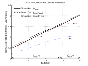
(a) $R_{\mathrm{fb}}=6$ Bits/Channel Realization

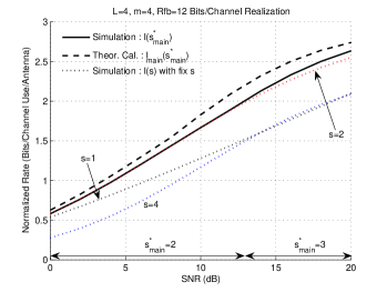
(b) $R_{\mathrm{fb}}=12$ Bits/Channel Realization

Figure 1: Total Throughput for Zero Forcing Beamforming

Fig. 1 gives the simulation results for the proposed scheme using zero-forcing. In the simulations, $L=m=4$. For simplicity, we assume that $\gamma_{1}=\gamma_{2}=\cdots=\gamma_{m}=1$ and $R_{1}=R_{2}=\cdots=R_{m}=R_{\mathrm{fb}}$. With these assumptions, the $s$ on-users can be randomly chosen from all the $m$ users. Without loss of generality, we assume that $A_{\mathrm{on}}\equiv\left\{1,\cdots,s\right\}$. Let $\mathcal{I}\left(s\right)=\sum_{i\in A_{\mathrm{on}}}\mathcal{I}_{i}.$ In Fig. 1, the solid lines are the simulations of $\mathcal{I}\left(s_{\mathrm{main}}^{*}\right)$ while the dashed lines are the theoretical calculation of $\mathcal{I}_{\mathrm{main}}\left(s_{\mathrm{main}}^{*}\right)$. The simulation results show that the optimal $s$ is a function of $\rho$ and $R_{\mathrm{fb}}$. For example, $s=1$ is optimal when $\rho\in\left[15,20\right]$dB and $R_{\mathrm{fb}}=6$ bits, while $s=3$ is optimal for the same SNR region as $R_{\mathrm{fb}}$ increases to 12 bits. The reason behind it is that the interference introduced by finite rate quantization is larger when $R_{\mathrm{fb}}$ is smaller: when $R_{\mathrm{fb}}$ is small, the base station needs to turn off some users to avoid strong interference as SNR gets very large.

We also compare our scheme with the schemes where the number of on-users is a presumed constant (independent of $\rho$ and $R_{\mathrm{fb}}$). The throughput of schemes with presumed $s$ is presented in dotted lines. From the simulation results, the throughput achieved by choosing appropriate $s$ is always better than or equals to that with presumed $s$. Specifically, compared to the scheme in [2] where $s=L=4$ always, our scheme achieves a significant gain at high SNR by turning off some users.

V Conclusion

This paper considers heterogeneous broadcast systems with a relatively small number of users. Asymptotic analysis where $L,m,s,R_{i}\rightarrow\infty$ linearly is employed to get insight into system design. Based on the asymptotic analysis, we derive the asymptotically optimal feedback strategy, propose a realistic on/off criterion, and quantify the spacial efficiency. The key observation is that the number of on-users should be appropriately chosen as a function of system parameters. Finally, a practical scheme is developed for finite dimensional systems. Simulations show that this scheme achieves a significant gain compared with previously studied schemes with presumed number of on-users.

References

• [1] M. Sharif and B. Hassibi, “On the capacity of mimo broadcast channels with partial side information,” Information Theory, IEEE Transactions on, vol. 51, no. 2, pp. 506–522, 2005.
• [2] N. Jindal, “MIMO broadcast channels with finite rate feedback,” IEEE Trans. Info. Theory, submitted.
• [3] W. Dai, Y. Liu, V. K. N. Lau, and B. Rider, “On the information rate of MIMO systems with finite rate channel state feedback using beamforming and power on/off strategy,” IEEE Trans. Info. Theory, submitted. [Online]. Available: http://arxiv.org/PS_cache/cs/pdf/0603/0603040.pdf
• [4] W. Dai, Y. Liu, and B. Rider, “Quantization bounds on Grassmann manifolds and applications to MIMO systems,” IEEE Trans. Info. Theory, Submitted. [Online]. Available: http://arxiv.org/PS_cache/cs/pdf/0603/0603039.pdf