Quantization Bounds on Grassmann Manifolds of Arbitrary Dimensions and MIMO Communications with Feedback${}^{{}^{*}}$

Abstract

This paper considers the quantization problem on the Grassmann manifold with dimension $n$ and $p$. The unique contribution is the derivation of a closed-form formula for the volume of a metric ball in the Grassmann manifold when the radius is sufficiently small. This volume formula holds for Grassmann manifolds with arbitrary dimension $n$ and $p$, while previous results are only valid for either $p=1$ or a fixed $p$ with asymptotically large $n$. Based on the volume formula, the Gilbert-Varshamov and Hamming bounds for sphere packings are obtained. Assuming a uniformly distributed source and a distortion metric based on the squared chordal distance, tight lower and upper bounds are established for the distortion rate tradeoff. Simulation results match the derived results. As an application of the derived quantization bounds, the information rate of a Multiple-Input Multiple-Output (MIMO) system with finite-rate channel-state feedback is accurately quantified for arbitrary finite number of antennas, while previous results are only valid for either Multiple-Input Single-Output (MISO) systems or those with asymptotically large number of transmit antennas but fixed number of receive antennas.

I Introduction

The Grassmann manifold $\mathcal{G}_{n,p}\left(\mathbb{L}\right)$ is the set of all $p$-dimensional planes (through the origin) of the $n$-dimensional Euclidean space $\mathbb{L}^{n}$, where $\mathbb{L}$ is either $\mathbb{R}$ or $\mathbb{C}$. It forms a compact Riemann manifold of real dimension $\beta p\left(n-p\right)$, where $\beta=1/2$ when $\mathbb{L}=\mathbb{R}/\mathbb{C}$ respectively. The Grassmann manifold provides a useful analysis tool for multi-antenna communications (also known as Multiple-Input Multiple-Output (MIMO) communication systems. For non-coherent MIMO systems, sphere packings on the $\mathcal{G}_{n,p}\left(\mathbb{L}\right)$ can be viewed as a generalization of spherical codes [1, 2, 3]. For MIMO systems with finite rate channel state feedback, the quantization of beamforming matrices is related to the quantization on the Grassmann manifold [4, 5, 6].

The basic quantization problems addressed in this paper are the sphere packing bounds and distortion rate tradeoff. A quantization is a mapping from the $\mathcal{G}_{n,p}\left(\mathbb{L}\right)$ into a subset of the $\mathcal{G}_{n,p}\left(\mathbb{L}\right)$, known as the code $\mathcal{C}$. Define $\delta\triangleq\delta\left(\mathcal{C}\right)$ as the minimum distance between any two elements in $\mathcal{C}$. The sphere packing bounds relate the size of a code and a given minimum distance $\delta$. Assuming a randomly distributed source on the $\mathcal{G}_{n,p}\left(\mathbb{L}\right)$ and a distortion metric, the distortion rate tradeoff is described by either the minimum expected distortion achievable for a given code size (distortion rate function) or the minimum code size required to achieve a particular expected distortion (rate distortion function).

For the sake of applications[4, 5, 6], the projection Frobenius metric (i.e. chordal distance) is employed throughout the paper although the corresponding analysis is also applicable to the geodesic metric [3]. For any two planes $P,Q\in\mathcal{G}_{n,p}\left(\mathbb{L}\right)$, the principle angles and the chordal distance between $P$ and $Q$ are defined as follows. Let $\mathbf{u}_{1}\in P$ and $\mathbf{v}_{1}\in Q$ be the unit vectors such that $\left|\mathbf{u}_{1}^{\dagger}\mathbf{v}_{1}\right|$ is maximal. Inductively, let $\mathbf{u}_{i}\in P$ and $\mathbf{v}_{i}\in Q$ be the unit vectors such that $\mathbf{u}_{i}^{\dagger}\mathbf{u}_{j}=0$ and $\mathbf{v}_{i}^{\dagger}\mathbf{v}_{j}=0$ for all $1\leq j<i$ and $\left|\mathbf{u}_{i}^{\dagger}\mathbf{v}_{i}\right|$ is maximal. The principle angles are defined as $\theta_{i}=\arccos\left|\mathbf{u}_{i}^{\dagger}\mathbf{v}_{i}\right|$ for $i=1,\cdots,n$ [7, 8]. The chordal distance between $P$ and $Q$ is defined as

$$d_{c}\left(P,Q\right)\triangleq\sqrt{\sum_{i=1}^{p}\sin^{2}\theta_{i}}.$$

The invariant measure on the $\mathcal{G}_{n,p}\left(\mathbb{L}\right)$ is defined as follows. Let $O\left(n\right)/U\left(n\right)$ be the group of $n\times n$ orthogonal/unitary matrices respectively. Let $\mathbf{A}\in O\left(n\right)/U\left(n\right)$ and $\mathbf{B}\in O\left(n\right)/U\left(n\right)$ when $\mathbb{L}=\mathbb{R}/\mathbb{C}$ respectively. An invariant measure $\mu$ on the $\mathcal{G}_{n,p}\left(\mathbb{L}\right)$ satisfies, for any measurable set $\mathcal{M}\subset\mathcal{G}_{n,p}\left(\mathbb{L}\right)$ and arbitrarily chosen $\mathbf{A}$ and $\mathbf{B}$,

$$\mu\left(\mathbf{A}\mathcal{M}\right)=\mu\left(\mathcal{M}\right)=\mu\left(\mathcal{M}\mathbf{B}\right).$$

The invariant measure defines the uniform distribution on the $\mathcal{G}_{n,p}\left(\mathbb{L}\right)$ [7].

With a metric and a measure defined on the $\mathcal{G}_{n,p}\left(\mathbb{L}\right)$, there are several bounds well known for sphere packings. Let $\delta$ be the minimum distance between any two elements of a code $\mathcal{C}$ and $B\left(\delta\right)$ be the metric ball of radius $\delta$ in the $\mathcal{G}_{n,p}\left(\mathbb{L}\right)$. If $K$ is any number such that $K\mu\left(B\left(\delta\right)\right)<1$, then there exists a code $\mathcal{C}$ of size $K+1$ and minimum distance $\delta$. This principle is called as the Gilbert-Varshamov lower bound [3], i.e.

$$\left|\mathcal{C}\right|>\frac{1}{\mu\left(B\left(\delta\right)\right)}.$$ (1)

On the other hand, $\left|\mathcal{C}\right|\mu\left(B\left(\delta/2\right)\right)\leq 1$ for any code $\mathcal{C}$. The Hamming upper bound captures this fact as[3]

$$\left|\mathcal{C}\right|\leq\frac{1}{\mu\left(B\left(\delta/2\right)\right)}.$$ (2)

These two bounds relate the code size and a given minimum distance $\delta$.

Distortion rate function gives another important property of quantization. Assume that $Q$ is a random plane uniformly distributed on the $\mathcal{G}_{n,p}\left(\mathbb{L}\right)$ and a distortion metric defined by the squared chordal distance $d_{c}^{2}$. The average distortion of a given $\mathcal{C}$ is

$$D\left(\mathcal{C}\right)\triangleq E_{Q}\left[\underset{P\in\mathcal{C}}{\min}\;d_{c}^{2}\left(P,Q\right)\right].$$ (3)

The distortion rate function gives the minimum average distortion for a given codebook size $K$, i.e.

$$D^{*}\left(K\right)=\underset{\mathcal{C}:\left|\mathcal{C}\right|=K}{\inf}\;D\left(\mathcal{C}\right).$$ (4)

There are several papers addressing quantization problems in the Grassmann manifold. The exact volume formula for a $B\left(\delta\right)$ in the $\mathcal{G}_{n,p}\left(\mathbb{C}\right)$ where $p=1$ is derived in [4]. An asymptotic volume formula for a $B\left(\delta\right)$ in the $\mathcal{G}_{n,p}\left(\mathbb{L}\right)$, where $p\geq 1$ is fixed and $n$ approaches infinity, is derived in [3]. Based on those volume formulas, the corresponding sphere packing bounds are developed in [5, 3]. Besides the sphere packing bounds, the rate distortion tradeoff is also treated in [9], where approximations to the distortion rate function are derived by the sphere packing bounds. However, the derived approximations are based on the volume formulas [3, 4] only valid for some special choices of $n$ and $p$, i.e. either $p=1$ or fixed $p\geq 1$ with asymptotic large $n$.

This paper derives quantization bounds for the Grassmann manifold with arbitrary $n$ and $p$ when the code size is large. An explicit volume formula for a metric ball in the $\mathcal{G}_{n,p}\left(\mathbb{L}\right)$ is derived when the radius is sufficiently small. Based on the derived volume formula, the sphere packing bounds are obtained. The distortion rate tradeoff is also characterized by establishment of tight lower and upper bounds. Simulation results match the derived bounds. As an application of the derived quantization bounds, the information rate of a MIMO system with finite rate channel state feedback is accurately quantified for abitrary finite number of antennas for the first time, while previous results are only valid for either Multiple-Input Single-Output (MISO) systems or those with asymptotically large number of transmit antennas but fixed number of receive antennas.

II Metric Balls in the $\mathcal{G}_{n,p}\left(\mathbb{L}\right)$

In this section, an explicit volume formula for a metric ball $B\left(\delta\right)$ in the $\mathcal{G}_{n,p}\left(\mathbb{L}\right)$ is derived. The volume formula is essential for the quantization bounds in Section III.

The volume calculation depends on the relationship between the measure and the metric defined on the $\mathcal{G}_{n,p}\left(\mathbb{L}\right)$. For the invariant measure $\mu$ and the chordal distance $d_{c}$, the volume of a metric ball $B\left(\delta\right)$ can be calculated by

$$\mu\left(B\left(\delta\right)\right)=\underset{\underset{\frac{\pi}{2}\geq\theta_{1}\geq\cdots\geq\theta_{p}\geq 0}{\sqrt{\sum_{i=1}^{p}\sin^{2}\theta_{i}}\leq\delta}}{\int\cdots\int}\;d\mu_{\mathbf{\theta}},$$ (5)

where $\theta_{1},\cdots,\theta_{p}$ are the principle angles and the differential form $d\mu_{\mathbf{\theta}}$ is given in [7, 10].

The following theorem expresses the volume formula as an exponentiation of the radius $\delta$.

Theorem 1

Let $B\left(\delta\right)$ be a ball of radius $\delta$ in $\mathcal{G}_{n,p}\left(\mathbb{L}\right)$. When $\delta\leq 1$,

$$\mu\left(B\left(\delta\right)\right)=\left\{\begin{array}[]{ll}c_{n,p,\beta}\delta^{p\left(n-p\right)}\left(1+o\left(\delta\right)\right)&\mathrm{if}\;\mathbb{L}=\mathbb{R}\\ c_{n,p,\beta}\delta^{2p\left(n-p\right)}&\mathrm{if}\;\mathbb{L}=\mathbb{C}\end{array}\right.,$$ (6)

where $\beta=1/2$ when $\mathbb{L}=\mathbb{R}/\mathbb{C}$ respectively and $c_{n,p,\beta}$ is a constant determined by $n$, $p$ and $\beta$. When $\mathbb{L}=\mathbb{C}$, $c_{n,p,2}$ can be explicitly calculated

$$c_{n,p,2}=\left\{\begin{array}[]{ll}\frac{1}{\left(np-p^{2}\right)!}\prod_{i=1}^{p}\frac{\left(n-i\right)!}{\left(p-i\right)!}&\mathrm{if}\;0<p\leq\frac{n}{2}\\ \frac{1}{\left(np-p^{2}\right)!}\prod_{i=1}^{n-p}\frac{\left(n-i\right)!}{\left(n-p-i\right)!}&\mathrm{if}\;\frac{n}{2}\leq p\leq n\end{array}\right..$$ (7)

When $\mathbb{L}=\mathbb{R}$, $c_{n,p,1}$ is given by

$$c_{n,p,1}=$$

$$\left\{\begin{array}[]{ll}\frac{V_{n,p,1}}{2^{p}}\underset{\underset{x_{1}\geq\cdots\geq x_{p}\geq 0}{\sum_{i=1}^{p}x_{i}\leq 1}}{\int\cdots\int}\left[\left|\prod_{i<j}^{p}\left(x_{i}-x_{j}\right)\right|\right.\\ \quad\quad\left.\prod_{i=1}^{p}\left(x_{i}^{\frac{1}{2}\left(n-2p+1\right)-1}dx_{i}\right)\right]&\mathrm{if}\;0<p\leq\frac{n}{2}\\ \frac{V_{n,n-p,1}}{2^{n-p}}\underset{\underset{x_{1}\geq\cdots\geq x_{n-p}\geq 0}{\sum_{i=1}^{n-p}x_{i}\leq 1}}{\int\cdots\int}\left[\left|\prod_{i<j}^{p}\left(x_{i}-x_{j}\right)\right|\right.\\ \quad\quad\left.\prod_{i=1}^{n-p}\left(x_{i}^{\frac{1}{2}\left(2p-n+1\right)-1}dx_{i}\right)\right]&\mathrm{if}\;\frac{n}{2}\leq p\leq n\end{array}\right.,$$ (12)

where

$$V_{n,p,1}=\prod_{i=1}^{p}\frac{A^{2}\left(p-i+1\right)A\left(n-p-i+1\right)}{2A\left(n-i+1\right)}$$

and

$$A\left(p\right)=\frac{2\pi^{p/2}}{\Gamma\left(\frac{p}{2}\right)}.$$

The proof of Theorem 1 is not included due to the length limit.

Theorem 1 provides an explicit volume approximation for real Grassmann manifolds and an exact volume formula for complex Grassmann manifolds when $\delta\leq 1$. Simulations show that this approximation remains good for relatively large $\delta$ (Fig. 1).

Theorem 1 is consistent with the previous results in [4] and [3], which pertain to special choices of $n$ and $p$ and are stated as follows.

Example 1

Consider the volume formula for a $B\left(\delta\right)$ in the $\mathcal{G}_{n,p}\left(\mathbb{C}\right)$ where $p=1$. It has been shown in [4] that

$$\mu\left(B\left(\delta\right)\right)=\delta^{2\left(n-1\right)}.$$

Theorem 1 is consistent with it where $\beta=2$ and $c_{n,1,2}=1$.

Example 2

When $p$ is fixed and $n\rightarrow+\infty$, the asymptotic volume formula for a $B\left(\delta\right)$ is given by Barg [3] as

$$\mu\left(B\left(\delta\right)\right)=\left(\frac{\delta}{\sqrt{p}}\right)^{\beta np+o\left(n\right)}.$$ (13)

On the other hand, Theorem 1 contains an asymptotic formula for $\mathbb{L}=\mathbb{C}$, $\delta\leq 1$, fixed $p$ and asymptotically large $n$ in the form

$$\mu\left(B\left(\delta\right)\right)=\left(\frac{\delta}{\sqrt{p}}\right)^{2p\left(n-p\right)+o\left(n\right)}.$$

This follows from (7) and Stirling’s approximation. Therefore, Theorem 1 is consistent with Barg’s formula (13).

Importantly though, Theorem 1 is distinct from the previous results of [4] and [3] in that it holds for arbitrary $n$ and $p$, $1\leq p\leq n$.

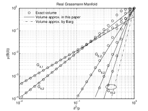
(a) Real Grassmann manifolds

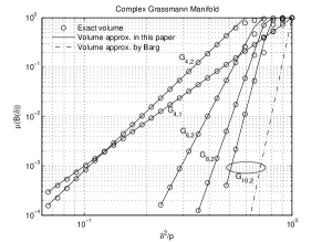
(b) Complex Grassmann manifolds

Figure 1: The volume of a metric ball in the Grassmann manifold

Fig. 1 compares the exact volume of a metric ball (5) and the volume evaluated by (6). For the volume approximation $c_{n,p,\beta}\delta^{\beta p\left(n-p\right)}$, the constant $c_{n,p,\beta}$ is calculated either by (7) if $\mathbb{L}=\mathbb{C}$ or by Monte Carlo numerical integral of (12) if $\mathbb{L}=\mathbb{R}$. Simulations show that the volume approximation is close to the exact volume when the radius of the metric ball is not large. We also compare our approximation with Barg’s approximation $\left(\delta/\sqrt{p}\right)^{\beta np}$ for $n=10$ and $p=2$ case. Simulations show that the exact volume and Barg’s approximation may not be in the same order while the approximation in this paper is more accurate.

III Quantization Bounds

Based on the volume formula given in Theorem 1, the sphere packing bounds are derived and the rate distortion tradeoff is characterized in this section.

The Gilbert-Varshamov and Hamming bounds on the $\mathcal{G}_{n,p}\left(\mathbb{L}\right)$ are given in the following corollary.

Corollary 1

When $\delta$ is sufficiently small, there exists a code in $\mathcal{G}_{n,p}\left(\mathbb{L}\right)$ with size $K$ and the minimum distance $\delta$ such that

$$c_{n,p,\beta}^{-1}\delta^{-\beta p\left(n-p\right)}\lesssim K.$$

For any code with the minimum distance $\delta$,

$$K\lesssim c_{n,p,\beta}^{-1}\left(\frac{\delta}{2}\right)^{-\beta p\left(n-p\right)}.$$

Here and throughtout, the symbol $\lesssim$ indicates that the inequality holds up to $\left(1+o\left(1\right)\right)$ error.

Proof:

The corollary follows by substituting the volume formula (6) into (1) and (2). ∎

The distortion rate function is characterized by establishing tight lower and upper bounds.

Theorem 2

Let $t=\beta p\left(n-p\right)$ be the number of the real dimensions of the Grassmann manifold $\mathcal{G}_{n,p}\left(\mathbb{L}\right)$. When $K$ is sufficiently large, the distortion rate function is bounded by

$$\frac{t}{t+2}\left(c_{n,p,\beta}K\right)^{-\frac{2}{t}}\lesssim D^{*}\left(K\right)\lesssim\frac{2\Gamma\left(\frac{2}{t}\right)}{t}\left(c_{n,p,\beta}K\right)^{-\frac{2}{t}}.$$ (14)

Due to the length limit, we only sketch the proof here. The lower bound is proved by an optimization argument. The key is to construct an ideal quantizer, which may not exist, to minimize the distortion. Suppose that there exists $K$ metric balls of the same radius $\delta_{0}$ covering the whole $\mathcal{G}_{n,p}\left(\mathbb{L}\right)$ completely without any overlap. Then the quantizer which maps each of those balls into its center gives the minimum distortion among all quantizers. Of course such a covering may not exist, provding a lower bound of the distortion rate function.

The upper bound is derived by characterizing the average distortion of the ensemble of random codes. Define a random code with size $K$ as $\mathcal{C}_{\mathrm{rand}}=\left\{P_{1},P_{2},\cdots,P_{K}\right\}$ where $P_{i}$’s are independently drawn from the uniform distribution on the $\mathcal{G}_{n,p}\left(\mathbb{L}\right)$. For any given $Q\in\mathcal{G}_{n,p}\left(\mathbb{L}\right)$, define $X_{i}\triangleq d_{c}^{2}\left(P_{i},Q\right)$ and $W_{K}\triangleq\min\left(X_{1},\cdots,X_{K}\right)=\underset{P_{i}\in\mathcal{C}_{\mathrm{rand}}}{\min}\;d_{c}^{2}\left(P_{i},Q\right)$. Since the codewords $P_{i}$’s $1\leq i\leq K$ are independently drawn from the uniform distribution on the $\mathcal{G}_{n,p}\left(\mathbb{L}\right)$, $X_{i}$’s $1\leq i\leq K$ are independent and identically distributed (i.i.d.) random variables with the cumulative distribution function (CDF) given by Theorem 1. According to $X_{i}$’s CDF, the CDF of $W_{K}$ can be calculated by extreme order statistics. We prove that for any given $Q\in\mathcal{G}_{n,p}\left(\mathbb{L}\right)$, $K^{\frac{t}{2}}\cdot\mathrm{E}_{W_{K}}\left[W_{K}\right]$ converges to $\frac{2\Gamma\left(\frac{2}{t}\right)}{t}c_{n,p,\beta}^{-\frac{2}{t}}$ as $K$ approaches infinity. Thus, $K^{\frac{t}{2}}\cdot\mathrm{E}_{Q}\left[\mathrm{E}_{W_{K}}\left[W_{K}\right]\right]=K^{\frac{t}{2}}\cdot\mathrm{E}_{\mathcal{C}_{\mathrm{rand}}}\left[D\left(\mathcal{C}_{\mathrm{rand}}\right)\right]$ converges to the same constant, providing an upper bound of $D^{*}\left(K\right)$.

It is worthy to point out that since the upper bound is corresponding to the ensemble of random codes, it is often used as an approximation to the distortion rate function in practice.

Fig. 2 compares the simulated distortion rate function with its lower bound and upper bound in (14). To simulate the distortion rate function, we use the max-min criterion [5] to design codes and use the minimum distortion of the designed codes as the distortion rate function. Simulations show that the bounds in (14) hold for large $K$. When $K$ is relatively small, the formula (14) can serve as good approximations to the distortion rate function as well. In addition, we compare our bounds with the approximation (the “x” markers) derived in [9]. While the approximation in [9] works for the case that $n=10$ and $p=2$ but doesn’t work when $n\leq 8$ and $p=2$, the bounds in (14) hold for arbitrary $n$ and $p$.

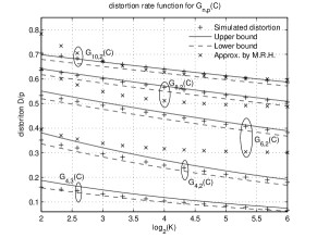
Figure 2: Bounds on the distortion rate function

IV Application to MIMO Systems with Finite Rate Channel State Feedback

As an application of the derived quantization bounds on the Grassmann manifold, this section discusses the information theoretical benefit of finite rate channel state feedback for MIMO systems using power on/off strategy. We will show that the benefit of the channel state feedback can be accurately characterized by the distortion of a quantization on the Grassmann manifold.

The effect of finite rate feedback on MIMO systems using power on/off strategy has been widely studied. MIMO systems with only one on-beam are discussed in [4, 5], where the performance analysis is derived by geometric arguments in the $\mathcal{G}_{n,1}\left(\mathbb{C}\right)$. For MIMO systems with multiple on-beams, many works, e.g. [9, 11, 12], employ Barg’s formula (13) for performance analysis, which is only valid for MIMO systems with asymptotically large number of antennas but fixed number of receive antennas. Valid for arbitrary MIMO systems, the loss in information rate is quantified for high SNR region in [13], which is hard to be generalized to other SNR regions. For all SNR regimes, a formula to calculate the information rate is proposed in [14] by letting the numbers of transmit and receive antennas and feedback rate approach infinity simultaneously. But this formula overestimates the performance in general.

The system model of a wireless communication system with $L_{T}$ transmit antennas, $L_{R}$ receive antennas and finite rate channel state feedback is given in Fig. 3. The information bit stream is encoded into the Gaussian signal vector $\mathbf{X}\in\mathbb{C}^{s\times 1}$ and then multiplied by the beamforming matrix $\mathbf{P}\in\mathbb{C}^{L_{T}\times s}$ to generate the transmitted signal $\mathbf{T}=\mathbf{PX}$, where $s$ is the dimension of the signal $\mathbf{X}$ satisfying $1\leq s\leq L_{T}$ and the beamforming matrix $\mathbf{P}$ satisfies $\mathbf{P}^{\dagger}\mathbf{P}=\mathbf{I}_{s}$. In power on/off strategy, $\mathrm{E}\left[\mathbf{X}\mathbf{X}^{\dagger}\right]=P_{\mathrm{on}}\mathbf{I}_{s}$ where $P_{\mathrm{on}}$ is a positive constant to denote the on-power. Assume that the channel $\mathbf{H}$ is Rayleigh flat fading, i.e., the entries of $\mathbf{H}$ are independent and identically distributed (i.i.d.) circularly symmetric complex Gaussian variables with zero mean and unit variance ($\mathcal{CN}\left(0,1\right)$) and $\mathbf{H}$ is i.i.d. for each channel use. Let $\mathbf{Y}\in\mathbb{C}^{L_{R}\times 1}$ be the received signal and $\mathbf{W}\in\mathbb{C}^{L_{R}\times 1}$ be the Gaussian noise, then

$$\mathbf{Y}=\mathbf{HPX}+\mathbf{W},$$

where $E\left[\mathbf{W}\mathbf{W}^{\dagger}\right]=\mathbf{I}_{L_{R}}$. We also assume that there is a beamforming codebook $\mathcal{B}=\left\{\mathbf{P}_{i}\in\mathbb{C}^{L_{T}\times s}:\right.$ $\left.\mathbf{P}_{i}^{\dagger}\mathbf{P}_{i}=\mathbf{I}_{s}\right\}$ declared to both the transmitter and the receiver before the transmission. At the beginning of each channel use, the channel state $\mathbf{H}$ is perfectly estimated at the receiver. A message, which is a function of the channel state, is sent back to the transmitter through a feedback channel. The feedback is error-free and rate limited. According to the channel state feedback, the transmitter chooses an appropriate beamforming matrix $\mathbf{P}_{i}\in\mathcal{B}$. Let the feedback rate be $R_{\mathrm{fb}}$bits/channel use. Then the size of the beamforming codebook $\left|\mathcal{B}\right|\leq 2^{R_{\mathrm{fb}}}$. The feedback function is a mapping from the set of channel state into the beamforming matrix index set, $\varphi:\;\left\{\mathbf{H}\right\}\rightarrow\left\{i:\;1\leq i\leq\left|\mathcal{B}\right|\right\}$. This section will quantify the corresponding information rate

$$\mathcal{I}=\underset{\mathcal{B}:\left|\mathcal{B}\right|\leq 2^{R_{\mathrm{fb}}}}{\max}\underset{\varphi}{\max}\;\mathrm{E}\left[\log\left|\mathbf{I}_{L_{R}}+P_{\mathrm{on}}\mathbf{H}\mathbf{P}_{\varphi\left(\mathbf{H}\right)}\mathbf{P}_{\varphi\left(\mathbf{H}\right)}^{\dagger}\mathbf{H}\right|\right],$$

where $P_{\mathrm{on}}=\rho/s$ and $\rho$ is the average received SNR.

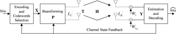
Figure 3: System model

Before discussing the finite rate feedback case, we consider the case that the transmitter has full knowledge of the channel state $\mathbf{H}$. In this setting, the optimal beamforming matrix is given by $\mathbf{P}_{\mathrm{opt}}=\mathbf{V}_{s}$ where $\mathbf{V}_{s}\in\mathbb{C}^{L_{T}\times s}$ is the matrix composed by the right singular vectors of $\mathbf{H}$ corresponding to the largest $s$ singular values [6]. The corresponding information rate is

$$\mathcal{I}_{\mathrm{opt}}=\mathrm{E}_{\mathbf{H}}\left[\sum_{i=1}^{s}\mathrm{ln}\left(1+P_{\mathrm{on}}\lambda_{i}\right)\right],$$ (15)

where $\lambda_{i}$ is the $i^{\mathrm{th}}$ largest eigenvalue of $\mathbf{H}\mathbf{H}^{\dagger}$. In [6], we derive an asymptotic formula to approximate a quantity of the form $\mathrm{E}_{\mathbf{H}}\left[\sum_{i=1}^{s}\ln\left(1+c\lambda_{i}\right)\right]$ where $c>0$ is a constant. Apply the asymptotic formula in [6]. $\mathcal{I}_{\mathrm{opt}}$ can be well approximated.

The effect of finite rate feedback can be characterized by the quantization bounds in the Grassmann manifold. For finite rate feedback, we define a suboptimal feedback function

$$i=\varphi\left(\mathbf{H}\right)\triangleq\underset{1\leq i\leq\left|\mathcal{B}\right|}{\arg\ \min}\;d_{c}^{2}\left(\mathcal{P}\left(\mathbf{P}_{i}\right),\mathcal{P}\left(\mathbf{V}_{s}\right)\right),$$ (16)

where $\mathcal{P}\left(\mathbf{P}_{i}\right)$ and $\mathcal{P}\left(\mathbf{V}_{s}\right)$ are the planes in the $\mathcal{G}_{L_{T},s}\left(\mathbb{C}\right)$ generated by $\mathbf{P}_{i}$ and $\mathbf{V}_{s}$ respectively. In [6], we show that this feedback function is asymptotically optimal as $R_{\mathrm{fb}}\rightarrow+\infty$ and near optimal when $R_{\mathrm{fb}}<+\infty$. With this feedback function and assuming that the feedback rate $R_{\mathrm{fb}}$ is large, it has been shown in [6] that

$$\mathcal{I} \approx \mathrm{E}_{\mathbf{H}}\left[\sum_{i=1}^{s}\ln\left(1+\eta_{\sup}P_{\mathrm{on}}\lambda_{i}\right)\right],$$ (17)

where

$$\eta_{\sup} \triangleq 1-\frac{1}{s}\underset{\mathcal{B}:\left|\mathcal{B}\right|\leq 2^{R_{\mathrm{fb}}}}{\inf}\;\mathrm{E}_{\mathbf{V}_{s}}\left[\underset{1\leq i\leq\left|\mathcal{B}\right|}{\ \min}\;d_{c}^{2}\left(\mathcal{P}\left(\mathbf{P}_{i}\right),\mathcal{P}\left(\mathbf{V}_{s}\right)\right)\right]$$ (18)

$$= 1-\frac{1}{s}D^{*}\left(2^{R_{\mathrm{fb}}}\right).$$

Thus, the difference between perfect beamforming case (15) and finite rate feedback case (17) is quantified by $\eta_{\sup}$, which depends on the distortion rate function on the $\mathcal{G}_{L_{T},s}\left(\mathbb{C}\right)$. Substitute quantization bounds (14) into (18) and apply the asymptotic formula in [6] for $\mathrm{E}_{\mathbf{H}}\left[\sum_{i=1}^{s}\ln\left(1+c\lambda_{i}\right)\right]$. Approximations to the information rate $\mathcal{I}$ are derived as functions of the feedback rate $R_{\mathrm{fb}}$.

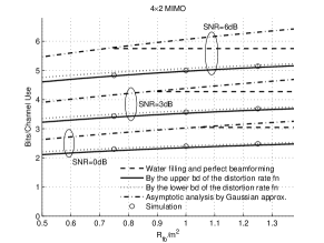
Figure 4: Performance of finite size beamforming codebook.

Simulations verify the above approximations. Let $m=\min\left(L_{T},L_{R}\right)$. Fig. 4 compares the simulated information rate (circles) and approximations as functions of $R_{\mathrm{fb}}/m^{2}$. The information rate approximated by the lower bound (solid lines) and the upper bound (dotted lines) in (14) are presented. As a comparison, we also include another performance approximation (dash-dot lines) proposed in [14], which is based on asymptotic analysis and Gaussian approximation. The simulation results show that the performances approximated by the bounds (14) match the actual performance almost perfectly and are much more accurate than the one in [14].

V Conclusion

This paper considers the quantization problem on the Grassmann manifold. Based on the explicit volume formula for a metric ball in the $\mathcal{G}_{n,p}\left(\mathbb{L}\right)$, the corresponding Gilbert-Varshamov and Hamming bounds are obtained. Assuming the uniform source distribution and the distortion defined by the squared chordal distance, the distortion rate function is characterized by establishing tight lower and upper bounds. As an application of these results, the information rate of a MIMO system with finite rate channel state feedback is accurately quantified for abitrary finite number of antennas for the first time.

References

- [1] D. Agrawal, T. J. Richardson, and R. L. Urbanke, “Multiple-antenna signal constellations for fading channels,” IEEE Trans. Info. Theory, vol. 47, no. 6, pp. 2618 – 2626, 2001.
- [2] Z. Lizhong and D. N. C. Tse, “Communication on the grassmann manifold: a geometric approach to the noncoherent multiple-antenna channel,” IEEE Trans. Info. Theory, vol. 48, no. 2, pp. 359 – 383, 2002.
- [3] A. Barg and D. Y. Nogin, “Bounds on packings of spheres in the Grassmann manifold,” IEEE Trans. Info. Theory, vol. 48, no. 9, pp. 2450–2454, 2002.
- [4] K. K. Mukkavilli, A. Sabharwal, E. Erkip, and B. Aazhang, “On beamforming with finite rate feedback in multiple-antenna systems,” IEEE Trans. Info. Theory, vol. 49, no. 10, pp. 2562–2579, 2003.
- [5] D. J. Love, J. Heath, R. W., and T. Strohmer, “Grassmannian beamforming for multiple-input multiple-output wireless systems,” IEEE Trans. Info. Theory, vol. 49, no. 10, pp. 2735–2747, 2003.
- [6] W. Dai, Y. Liu, V. K. N. Lau, and B. Rider, “On the information rate of MIMO systems with finite rate channel state feedback using beamforming and power on/off strategy,” IEEE Trans. Info. Theory, submitted.
- [7] A. T. James, “Normal multivariate analysis and the orthogonal group,” Ann. Math. Statist., vol. 25, no. 1, pp. 40 – 75, 1954.
- [8] J. H. Conway, R. H. Hardin, and N. J. A. Sloane, “Packing lines, planes, etc., packing in Grassmannian spaces,” Exper. Math., vol. 5, pp. 139–159, 1996.
- [9] B. Mondal, R. W. H. Jr., and L. W. Hanlen, “Quantization on the Grassmann manifold: Applications to precoded MIMO wireless systems,” in Proc. IEEE International Conference on Acoustics, Speech, and Signal Processing (ICASSP), 2005, pp. 1025–1028.
- [10] M. Adler and P. v. Moerbeke, “Integrals over Grassmannians and random permutations,” ArXiv Mathematics e-prints, 2001.
- [11] D. J. Love and J. Heath, R. W., “Limited feedback unitary precoding for orthogonal space-time block codes,” IEEE Trans. Signal Processing, vol. 53, no. 1, pp. 64 – 73, 2005.
- [12] ——, “Limited feedback precoding for spatial multiplexing systems,” in IEEE Global Telecommunications Conference (GLOBECOM), vol. 4, 2003, pp. 1857– 1861.
- [13] J. C. Roh and B. D. Rao, “MIMO spatial multiplexing systems with limited feedback,” in Proc. IEEE International Conference on Communications (ICC), 2005.
- [14] W. Santipach and M. L. Honig, “Asymptotic performance of MIMO wireless channels with limited feedback,” in Proc. IEEE Military Comm. Conf., vol. 1, 2003, pp. 141– 146.