Bell Inequality Based on Peres-Horodecki Criterion

Abstract

We established a physically utilizable Bell inequality based on the Peres-Horodecki criterion. The new quadratic probabilistic Bell inequality naturally provides us a necessary and sufficient way to test all entangled two-qubit or qubit-qutrit states including the Werner states and the maximally entangled mixed states.

One of the most striking features for quantum mechanics that differs from classical theory is the entanglement or the nonlocality. Arising from the EPR paradox (1935)Einstein , the local hidden variable theory (LHVT) was exploited by Bell and led to the appearance of Bell inequality (1964)Bell . The importance of the Bell inequality is not extravagance. It is at the heart of the study of quantum nonlocality, and makes it possible for the first time to distinguish experimentally between a local hidden variable model and quantum mechanics. The original Bell inequality is not suitable for realistic experimental verification. Later on, the Clauser-Horne-Shimony-Holt (CHSH) inequality (1969)Clauser was formulated, and it was a more amenable version for experimental tests and studied the correlations between two maximally entangled spin-1/2 particles.

For decades, quantum nonlocality has been tightly related to the foundations of quantum mechanics, particularly to quantum inseparability and the violation of Bell inequalities. Violation of Bell inequalities not only tells us something fundamental about Nature but also has practical applications. For instances, as implied by Ekert the eavesdropping in the quantum cryptography communication can be detected by checking the CHSH inequality (1991)Ekert ; also Barrett et al. have described that testing particular nonlocal quantum correlations allows two parties to distribute a secret key securely, the security of the scheme stems from violation of a Bell inequality and in such a way that the security is guaranteed by the non-signaling principle alone (2005)Barrett .

Despite more than four decades of active research and a vast number of publications on the fascinating subject of Bell inequality, there are still many questions that remain open. The CHSH inequality simply but effectively illustrates the distinct nonlocal correlation character of quantum world. Any entangled two-qubit pure state can always be detected by the CHSH inequality via its violation Gisin . However, in the real world some states appear in pure forms but more in mixed-state forms. In particular, for a class of Werner states (2000)Nielson which are used to depict the effect of noises, there exists a range where the CHSH inequality becomes blind Werner0 ; Horodecki0 . Very recently in a significant Festschrift in honor of Abner Shimony, Gisin has reviewed some of the many open questions about Bell inequalities Gisin2007 . Fifteen open fundamental questions have been listed, among which the third one is whether we can find an inequality that is more efficient than the CHSH inequality for testing the Werner states. Or more generally, one may ask: Is there a universal Bell inequality, which is violated by all of the entangled two-qubit states including the Werner states? Such a question seems to be some puzzling for when referring to Bell inequality it often concerns about the obeisance of LHVT or the violation of quantum theory, rather than the inseparability of physical states. Yet, the increasing importance of the nonlocal correlation characters in the Quantum Information and Communication revolution has led us to extend the Bell inequality and test the inseparability as well; namely, it is necessary to generalize the original spirit of Bell inequality for distinguishing LHVT from quantum theory to a new problem of distinguishing all separable states from all inseparable ones.

In this Letter we show that there exists such an efficient Bell inequality to ameliorate the above situation, and it originates naturally from the pioneer works of Peres and Horodecki family. A decade ago a sufficient and necessary criterion for detecting quantum inseparability in a two-qubit or qubit-qutrit system was presented mathematically by Peres (1996)Peres and the Horodecki family (1996)Horodecki , nowadays known as the Peres-Horodecki criterion of positivity under partial transpose (PH criterion or PPT criterion). In 2003, Yu et al. made a remarkable progress that they established a three-setting Bell-type inequality from the viewpoint of indeterminacy relation of complementary local orthogonal observables, and proved that such an inequality had the advantage of being a sufficient and necessary criterion of separability with the help of PH criterion Yu(2003) . Since it is not easy to operate physically the partial transpose to a subsystem, in the Letter we transform the PH criterion into an equivalent physically utilizable Bell-inequality form, and the new established quadratic probabilistic Bell inequality naturally provides us a necessary and sufficient way to test all entangled two-qubit or qubit-qutrit states including the Werner states.

Let us firstly analyze the paramount CHSH inequality from the viewpoint of the projective measurements, and then turn to our main result. The CHSH inequality reads

$$I_{CHSH} = \langle A_{1}B_{1}\rangle_{\rho}+\langle A_{1}B_{2}\rangle_{\rho}+\langle A_{2}B_{1}\rangle_{\rho}-\langle A_{2}B_{2}\rangle_{\rho}$$ (1)

$$\leq 2,$$

where $\langle A_{i}B_{j}\rangle_{\rho}\equiv Q_{ij}={\rm Tr}[\rho\;(\hat{a}_{i}\cdot\vec{\sigma}^{A})(\hat{b}_{j}\cdot\vec{\sigma}^{B})]$ known as the so-called correlation functions, $\rho$ is the two-qubit state shared by A and B, $\vec{\sigma}$ is the Pauli matrix vector, $\hat{a}_{1}$ and $\hat{a}_{2}$ are the unit vectors for the first and the second measurements performed to the subsystem A respectively and so do $\hat{b}_{1}$ and $\hat{b}_{2}$ for the subsystem B. According to the measurement language, the correlation functions can be expressed in terms of joint probabilities as $\langle A_{i}B_{j}\rangle_{\rho}=\sum_{m=0}^{1}\sum_{n=0}^{1}(-1)^{m+n}P(A_{i}=m,B_{j}=n)$, with the joint probability $P(A_{i}=m,B_{j}=n)=\mathrm{Tr}[\rho\ \hat{\mathcal{P}}(A_{i}=m)\otimes\hat{\mathcal{P}}(B_{j}=n)]$, and the projector $\hat{\mathcal{P}}(A_{i}=m)=\frac{1}{2}[1+(-1)^{m}\ \hat{a}_{i}\cdot\vec{\sigma}^{A}]$. Thus all relevant polarization vectors $\{\hat{a}_{1},-\hat{a}_{1},\hat{a}_{2},-\hat{a}_{2}\}$ and $\{\hat{b}_{1},-\hat{b}_{1},\hat{b}_{2},-\hat{b}_{2}\}$ in the Bloch spheres of each subsystem always locate on the same plane embraced by a great circle [see Fig. 1(a)] so that such projective measurements cannot acquire any information outside the plane. This may be the reason of the invalidation of the CHSH inequality for the whole mixed states.

To overcome this flaw, we adopt Positive Operator-Valued Measure (POVM). An operator $E_{m}$ is a POVM element if it is a positive operator satisfying $\sum_{m}E_{m}=1$ and then the complete set $\{E_{m}\}$ form a POVM (2000)Nielson ; Preskill . Gisin and Popescu have conjectured that more information is extractable if one adopts a special class of vectors, such as $(0,0,1)$, $(\sqrt{8},0,-1)/3$, $(-\sqrt{2},\sqrt{2},-1)/3$, $(-\sqrt{2},-\sqrt{2},-1)/3$, which occupy the four vertices of a regular tetrahedron inscribed in the three-dimensional Bloch sphere Gisin(1999) . One may observe that these four unit vectors sum up to zero, thus it allows us to introduce the following POVM operators:

$$\tilde{F}_{i}^{A}=UF_{i}^{A}{U^{\dagger}},\quad\quad\quad\;\;\;\; \tilde{F}_{i}^{B}=VF_{i}^{B}{V^{\dagger}},$$ (2)

$$F_{i}^{A}=(1+\hat{n}_{i}^{A}\cdot\vec{\sigma}^{A})/4,\quad F_{i}^{B}=(1+\hat{n}_{i}^{B}\cdot\vec{\sigma}^{B})/4,$$

where $U$ and $V$ are the general $SU(2)$ transformations for subsystems A and B respectively, and for simplicity, the four unit vectors $\hat{n}_{i}$ [see Fig. 1(b)] that form a tetrahedron are chosen as

$$\hat{n}_{1}=(1,1,1)/\sqrt{3},\;\;\;\;\;\;\;\;\hat{n}_{2}=(1,-1,-1)/\sqrt{3},$$

$$\hat{n}_{3}=(-1,1,-1)/\sqrt{3},\;\;\hat{n}_{4}=(-1,-1,1)/\sqrt{3}.$$ (3)

By the way, such a POVM realization has been applicable successfully as a minimal measurement scheme for a single-qubit tomography Rehacek(2004) .

Accordingly, the sixteen elements $\tilde{F}_{i}^{A}\otimes\tilde{F}_{j}^{B}$ form a POVM for the composite A-B system and $\langle\tilde{F}^{A}_{i}\tilde{F}^{B}_{j}\rangle_{\rho}={\rm Tr}[\rho\;\tilde{F}^{A}_{i}\otimes\tilde{F}^{B}_{j}]\equiv P_{ij}^{AB}$ denotes the joint probability of the joint measurement $\tilde{F}^{A}_{i}\otimes\tilde{F}^{B}_{j}$ on the state $\rho$. These sixteen joint probabilities sum up to one and will be used to construct a Bell inequality subsequently. Our main result is the following Theorem.

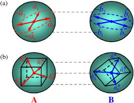
Figure 1: (Color online) (a) In the Bloch sphere of a single qubit, the four polarized unit vectors $\{\hat{a}_{1},-\hat{a}_{1},\hat{a}_{2},-\hat{a}_{2}\}$ or $\{\hat{b}_{1},-\hat{b}_{1},\hat{b}_{2},-\hat{b}_{2}\}$ employed in the projective measurements of the CHSH-inequality lie on the plane embraced by a great circle; (b) the four unit vectors $\{\hat{n}_{i}\}$ employed in the POVM measurements of the PH-inequality uniformly lie on the Bloch sphere and their endpoints occupy exactly the four vertices of a regular tetrahedron. (Note: $\hat{n}_{i}^{A}$ and $\hat{n}_{j}^{B}$ have been rotated by $U$ and $V$ respectively in the figure.)

Theorem: The Peres-Horodecki criterion for qubit-qubit system is equivalent to the following quadratic Bell-type inequality:

$$I_{PH}=Y_{1}^{2}+Y_{2}^{2}-Y_{3}^{2}\leq 0,$$ (4)

where $Y_{i}$’s are linear combinations of the sixteen joint probabilities $P_{ij}^{AB}$, and $I_{PH}$ denotes Bell inequality induced from the PH criterion, alternatively one may call it the PH inequality.

Proof. First we write an arbitrary projector for $AB$ system into the form $\hat{\cal P}_{AB}=(U\otimes V)|\Phi\rangle\langle\Phi|(U\otimes V)^{\dagger}$, where

$$|\Phi\rangle=\sin\xi|0\rangle_{A}\otimes|0\rangle_{B}+\cos\xi|1\rangle_{A}\otimes|1\rangle_{B},$$ (5)

is a two-qubit pure state in the Schmidt decomposition form, the unitary transformations $U$ and $V$ act on the parties $A$ and $B$ respectively, the angle $\xi$ is related to the Schmidt coefficient, and $|0\rangle=(1,0)^{T}$, $|1\rangle=(0,1)^{T}$ are the standard spin-1/2 bases.

Let $\rho$ be the state shared by A and B. The nonnegativity of the density matrix $\rho$ requires that

$$\mathrm{Tr}(\rho\ \hat{\cal P}_{AB})=\mathrm{Tr}[\rho\ (U\otimes V)|\Phi\rangle\langle\Phi|(U\otimes V)^{\dagger}]\geq 0.$$ (6)

On the other hand, the PH criterion states that $\rho$ is separable if and only if its partial transpose $\rho^{T_{B}}$ is nonnegative, i.e., $\mathrm{Tr}(\rho^{T_{B}}\hat{\cal P}_{AB})\geq 0$, or more generally $\mathrm{Tr}[\rho^{T_{B}}\;(U^{A}\otimes U^{B})\hat{\cal P}_{AB}(U^{A}\otimes U^{B})^{\dagger}]\geq 0$. By using $\mathrm{Tr}[\rho^{T_{B}}\;(U^{A}\otimes U^{B})\hat{\cal P}_{AB}(U^{A}\otimes U^{B})^{\dagger}]=\mathrm{Tr}[\rho\ [(U^{A}\otimes U^{B})\hat{\cal P}_{AB}(U^{A}\otimes U^{B})^{\dagger}]^{T_{B}}]=\mathrm{Tr}[\rho\ (U^{A}U\otimes(U^{B}V)^{{\dagger}T_{B}})(|\Phi\rangle\langle\Phi|)^{T_{B}}((U^{A}U)^{\dagger}\otimes(U^{B}V)^{T_{B}})]$, and selecting $U^{A}=I$, $U^{B}=(VV^{T_{B}})^{\dagger}$, one arrives at an equivalent expression for the PH criterion as

$$\mathrm{Tr}[\rho\ (U\otimes V)(|\Phi\rangle\langle\Phi|)^{T_{B}}(U\otimes V)^{\dagger}]\geq 0.$$ (7)

We now combine Eqs. (6) and (7) together to build the quadratic Bell inequality. With the help of $|0\rangle_{S}\langle 0|=1/2+\sqrt{3}(F^{S}_{1}+F^{S}_{4}-F^{S}_{2}-F^{S}_{3})/2$, $|0\rangle_{S}\langle 1|=\sqrt{3}[(1+i)(F^{S}_{1}-F^{S}_{4})+(1-i)(F^{S}_{2}-F^{S}_{3})]/2$, $|1\rangle_{S}\langle 1|=1-|0\rangle\langle 0|$, $|1\rangle_{S}\langle 0|=(|0\rangle\langle 1|)^{\dagger}$, where $S=A,B$, we may expand $|\Phi\rangle\langle\Phi|$ in terms of POVM operators as

$$|\Phi\rangle\langle\Phi| = (\sin 2\xi\;\hat{X}_{1}-\cos 2\xi\;\hat{X}_{2}+\hat{X}_{3})/4,$$ (8)

where $\hat{X}_{1}=2(|0\rangle_{A}\langle 1|\otimes|0\rangle_{B}\langle 1|+|1\rangle_{A}\langle 0|\otimes|1\rangle_{B}\langle 0|)=6(F_{1}^{A}F_{2}^{B}+F_{2}^{A}F_{1}^{B}+F_{3}^{A}F_{4}^{B}+F_{4}^{A}F_{3}^{B}-F_{1}^{A}F_{3}^{B}-F_{3}^{A}F_{1}^{B}-F_{2}^{A}F_{4}^{B}-F_{4}^{A}F_{2}^{B})$, $\hat{X}_{2}=2(|0\rangle_{A}\langle 0|\otimes|0\rangle_{B}\langle 0|-|1\rangle_{A}\langle 1|\otimes|1\rangle_{B}\langle 1|)=\sqrt{3}(F_{1}^{A}+F_{4}^{A}-F_{2}^{A}-F_{3}^{A}+F_{1}^{B}+F_{4}^{B}-F_{2}^{B}-F_{3}^{B})$, $\hat{X}_{3}=2(|0\rangle_{A}\langle 0|\otimes|0\rangle_{B}\langle 0|+|1\rangle_{A}\langle 1|\otimes|1\rangle_{B}\langle 1|)=1+3(F_{1}^{A}F_{1}^{B}+F_{2}^{A}F_{2}^{B}+F_{3}^{A}F_{3}^{B}+F_{4}^{A}F_{4}^{B}+F_{1}^{A}F_{4}^{B}+F_{4}^{A}F_{1}^{B}+F_{2}^{A}F_{3}^{B}+F_{3}^{A}F_{2}^{B}-F_{1}^{A}F_{2}^{B}-F_{2}^{A}F_{1}^{B}-F_{1}^{A}F_{3}^{B}-F_{3}^{A}F_{1}^{B}-F_{2}^{A}F_{4}^{B}-F_{4}^{A}F_{2}^{B}-F_{3}^{A}F_{4}^{B}-F_{4}^{A}F_{3}^{B})$. Similarly, we have $(|\Phi\rangle\langle\Phi|)^{T_{B}}=(\sin 2\xi\;\hat{Y}_{1}-\cos 2\xi\;\hat{Y}_{2}+\hat{Y}_{3})/4$, with $\hat{Y}_{i}=\hat{X}_{i}^{T_{B}}$. Due to $(F_{1}^{B})^{T_{B}}=1/2-F_{3}^{B}$, $(F_{2}^{B})^{T_{B}}=1/2-F_{4}^{B}$, $(F_{3}^{B})^{T_{B}}=1/2-F_{1}^{B}$, $(F_{4}^{B})^{T_{B}}=1/2-F_{2}^{B}$, one may easily have $\hat{Y}_{1}=\hat{X}_{1}^{T_{B}}=6(F_{1}^{A}F_{1}^{B}+F_{2}^{A}F_{2}^{B}+F_{3}^{A}F_{3}^{B}+F_{4}^{A}F_{4}^{B}-F_{1}^{A}F_{4}^{B}-F_{4}^{A}F_{1}^{B}-F_{2}^{A}F_{3}^{B}-F_{3}^{A}F_{2}^{B})$, $\hat{Y}_{2}=\hat{X}_{2}^{T_{B}}=\hat{X}_{2}$ and $\hat{Y}_{3}=\hat{X}_{3}^{T_{B}}=\hat{X}_{3}$.

Substituting Eq. (8) into Eq. (6), and using $\sin 2\xi=2t/(1+t^{2})$, $\cos 2\xi=(1-t^{2})/(1+t^{2})$ with $t=\tan\xi$, one then gets an algebraic quadratic inequality with respect to $t$ as

$$(X_{2}+X_{3})\ t^{2}+2X_{1}\ t+(X_{3}-X_{2})\geq 0,$$

where $X_{i}=\mathrm{Tr}[\rho\ (U\otimes V)\hat{X}_{i}(U\otimes V)^{\dagger}]$; since it is valid for any $t$, thus the coefficient of $t^{2}$ must be nonnegative, namely the nonnegativity of the density matrix $\rho$ ensures that $X_{2}+X_{3}\geq 0$. Similarly, Eq. (7) yields $a\ t^{2}+b\ t+c\geq 0$, where $a=Y_{2}+Y_{3}$, $b=2Y_{1}$, $c=Y_{3}-Y_{2}$, and $Y_{i}=\mathrm{Tr}[\rho\ (U\otimes V)\hat{Y}_{i}(U\otimes V)^{\dagger}]$ can be expressed in terms of the joint probabilities $P_{ij}^{AB}$ as: $Y_{1}=6(P_{11}^{AB}+P_{22}^{AB}+P_{33}^{AB}+P_{44}^{AB}-P_{14}^{AB}-P_{41}^{AB}-P_{23}^{AB}-P_{32}^{AB})$, $Y_{2}=\sqrt{3}(P_{1}^{A}+P_{4}^{A}-P_{2}^{A}+P_{3}^{A}+P_{1}^{B}+P_{4}^{B}-P_{2}^{B}+P_{3}^{B})$, $Y_{3}=1+3(P_{11}^{AB}+P_{22}^{AB}+P_{33}^{AB}+P_{44}^{AB}+P_{14}^{AB}+P_{41}^{AB}+P_{23}^{AB}+P_{32}^{AB}-P_{12}^{AB}-P_{21}^{AB}-P_{13}^{AB}-P_{31}^{AB}-P_{24}^{AB}-P_{42}^{AB}-P_{34}^{AB}-P_{43}^{AB})$, here the single probabilities satisfy $P_{i}^{A}=\sum_{j}P_{ij}^{AB}$ and $P_{j}^{B}=\sum_{i}P_{ij}^{AB}$. The PH criterion demands the quadratic inequality $a\ t^{2}+b\ t+c\geq 0$ holds for all $t$, so one must have (i) $a\geq 0$ and (ii) $b^{2}-4ac\geq 0$. The first condition is automatically satisfied because $a=Y_{2}+Y_{3}=X_{2}+X_{3}$, while the second condition leads to the needed quadratic Bell inequality as shown in (4). This ends the proof.

The PH inequality naturally provides us a necessary and sufficient way to test all entangled two-qubit states. To see this point clearly we would like to provide two explicit examples as follows.

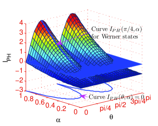
Figure 2: (Color online) The maximal violation of the PH inequality $I_{PH}$ for the general Werner state has been plotted. Specifically, the curves for both the maximal violation of the usual Werner state $I_{PH}(\pi/4,\alpha)$ and the boundary of sparable states $I_{PH}(\theta,\alpha)=0$ [ i.e., $(1+2|\sin 2\theta|)\alpha-1=0$] have been marked out (see the blue lines).

Example 1: The Werner State. The general two-qubit Werner state reads

$$\rho_{GW}=\alpha|\psi(\theta)\rangle\langle\psi(\theta)|+(1-\alpha)1\!\!1/4,$$ (9)

where $|\psi(\theta)\rangle=\cos\theta|00\rangle+\sin\theta|11\rangle$, $1\!\!1$ is a $4\times 4$ unit matrix, $\alpha\in[0,1]$, and $\theta\in[0,\pi]$. When the parameter $\theta=\pi/4$ it reduces to the usual Werner state $\rho_{W}$, and when the parameter $\alpha=1$ it reduces to the pure state $|\psi(\theta)\rangle$. It is well known that the state $\rho_{W}$ is separable if $\alpha\leq 1/3$ and nonseparable if $\alpha>1/3$. However the CHSH inequality can be violated only for the region $\alpha\in(1/\sqrt{2},1]$, in other words, the Werner state $\rho_{W}$ is still entangled within the region $\alpha\in(1/3,1/\sqrt{2}]$ but the CHSH inequality fails to detect its inseparability. For the general Werner state $\rho_{GW}$, we have the maximum of the PH inequality as $I_{PH}^{\max}(\theta,\alpha)=[(1+2|\sin 2\theta|)\alpha-1](1+\alpha)$, see Fig. 2. For pure states $|\psi(\theta)\rangle$, one has $I_{PH}^{\max}(\theta,\alpha=1)=4|\sin 2\theta|$. For $\theta=\pi/4$, $I_{PH}^{\max}(\theta=\pi/4,\alpha)=(3\alpha-1)(1+\alpha)$, namely, the Werner state $\rho_{W}$ is violated for the whole nonseparable region of $\alpha\in(1/3,1]$.

Example 2: The Maximally Entangled Mixed State. This state was predicted by White et al. and had the following explicit form White(2002)

$$\rho_{m}=\left(\begin{array}[]{cccc}g(\gamma)&0&0&\frac{\gamma}{2}\\ 0&1-2g(\gamma)&0&0\\ 0&0&0&0\\ \frac{\gamma}{2}&0&0&g(\gamma)\end{array}\right),$$ (10)

with $g(\gamma)=\gamma/2$ for $2/3\leq\gamma\leq 1$ and $g(\gamma)=1/3$ for $0\leq\gamma<2/3$. The state is entangled for all nonzero $\gamma$ due to its concurrence Munro(2001) equals to $\gamma$. It is easy to verify that the PH inequality for such states has its maximal violation as $I_{PH}^{\max}(\gamma)=4\gamma^{2}$.

The above approach can be easily generalized to a qubit-qutrit system and one still obtains the same quadratic form of Bell inequality as in (4), because the projector $\hat{\cal P}_{AB}$ still shares the same form for arbitrary qubit-qutrit systems. The POVM for subsystem A remains the same as shown in Eq. (2), while the POVM for subsystem B is extended to $\tilde{F}_{i}^{B}=VF_{i}^{B}{V^{\dagger}}$, $(i=1,2,\cdots,9)$, where $V$ is a general $SU(3)$ transformation, $F^{B}_{i}=(1/9)(1+\sqrt{3}/2\ \hat{v}_{i}\cdot\vec{\lambda})$, $\vec{\lambda}=(\lambda_{1},\lambda_{2},\cdots,\lambda_{8})$ is the vector of $SU(3)$ Gell-Mann matrices, the factor $\sqrt{3}/2$ is introduced to guarantee the nonnegativity, and the nine unit vectors $\hat{v}_{i}$’s distribute uniformly in the eight-dimensional Bloch space. Following the similar spirit as in the proof, one may obtain the quadratic Bell inequality (4) for the qubit-qutrit system but with different $Y_{i}$’s, which are linear combinations of the $4\times 9=36$ joint probabilities $P_{ij}^{AB}$ of the qubit-qutrit system.

It is worthy to mention that the CHSH inequality possesses two evident properties: (i) it is a two-setting inequality based on the standard Bell experiment. By a standard Bell experiment, we mean one in which each local observer is given a choice between two dichotomic observables zukowski2 ; zukowski1 ; weinfurter ; werner ; (ii) it is a linear inequality. In 2002, two research teams independently developed Bell inequalities for two high-dimensional systems: the first one is a Clauser-Horne type (probability) inequality for two qutrits JLC2 ; and the second one is a CHSH type (correlation) inequality to two arbitrary $d$-dimensional systems CGLMP , now known as the Collins-Gisin-Linden-Massar-Popescu (CGLMP) inequalities. The CGLMP inequality is a two-setting inequality by the virtue of the standard Bell experiment with possible $d$-outcomes, which includes the CHSH inequality as a special case. The tightness of the CGLMP inequality has been demonstrated in Ref. LM , therefore it is impossible to improve the CHSH inequality to be a sufficient and necessary criterion of separability within the framework of the standard Bell experiment. There are no physical reasons that a Bell inequality must be linear. The PH inequality does not inherit the above two properties and it is a quadratic four-setting inequality.

In conclusion, we have established a physically utilizable Bell inequality based on the Peres-Horodecki criterion. The new quadratic probabilistic Bell inequality naturally provides us a necessary and sufficient way to test all entangled two-qubit or qubit-qutrit states including the Werner states. The PH inequality is more efficient than the CHSH inequality. For the crucial role of the CHSH inequality in the previous eavesdropping detection in the Ekert’s quantum cryptography protocol, it is instructive to mention that the PH inequality may provide a more robust approach for detecting the eavesdropping particularly in the presence of noises. In addition, if a Bell inequality is violated by any entangled states, such a wisdom can be used to define the degree of entanglement $P_{E}$; for two qubits, alternatively one may define $P_{E}={\rm Max}\{0,I_{PH}^{\max}/4\}$, which is monotonic to the concurrence Wootters(1998) .

We thank Y. C. Liang for his valuable discussion. This work is supported by NSF of China (Grant No. 10605013) and Program for New Century Excellent Talents in University.

References

(1)A. Einstein, B. Podolsky, and N. Rosen,
Phys. Rev. 47, 777 (1935).
(2)J. S. Bell, Physics (Long Island City, N.Y.)
1, 195 (1964).
(3)J. F. Clauser, M. A. Horne, A. Shimony, and
R. A. Holt, Phys. Rev. Lett. 23, 880 (1969).
(4)A. K. Ekert, Phys. Rev. Lett. 67, 661
(1991).
(5)J. Barrett, L. Hardy, and A. Kent, Phys. Rev. Lett. 95, 010503
(2005).
(6)
N. Gisin, Phys. Lett. A 154, 201 (1991); N. Gisin and A.
Peres, Phys. Lett. A 162, 15-17 (1992); S. Popescu and D.
Rohrlich, Phys. Lett. A 166, 293 (1992).
(7)M. A. Nielsen and I. L. Chuang, Quantum Computation and
Quantum Information (Cambridge University Press, Cambridge,
England, 2000).
(8) R. F. Werner, Phys. Rev. A 40, 4277 (1989).
(9) R. Horodecki, P. Horodecki, and M.
Horodecki, Phys. Lett. A 200, 340 (1995); R. Horodecki,
Phys. Lett. A 210, 223 (1996).
(10) N. Gisin, arXiv:quant-ph/0702021.
(11)A. Peres, Phys. Rev. Lett. 77, 1413 (1996).
(12)M. Horodecki, P. Horodecki, and R.
Horodecki, Phys. Lett. A 223, 1 (1996).
(13)S. Yu, J. W. Pan, Z. B. Chen, and Y. D. Zhang,
Phys. Rev. Lett. 91, (2003) 217903.
(14) J. Preskill, Lecture notes for Physics299: Quantum Information and
Computation,
California Institute of Technology, 1998.
(15) N. Gisin, and S. Popescu, Phys. Rev. Lett.
83, 432 (1999); S. Ghosh, A. Roy, and U. Sen, Phys. Rev. A
63, 014301 (2000).
(16) J. Řeháček, B. G Englert, and D. Kaszlikowski,
Phys. Rev. A 70, 052321 (2004).
(17)A. G. White, D. F. V. James, W. J. Munro, and P. G. Kwiat, Phys. Rev. A 65, 012301
(2002).
(18)W. J. Munro, K. Nemoto, and A. G. White, J. Mod. Opt. 48, 1239
(2001).
(19)
M. Żukowski, Č. Brukner, W. Laskowski, and M. Wiesniak,
Phys. Rev. Lett. 88, 210402 (2002).
(20)
M. Żukowski, and Č. Brukner, Phys. Rev. Lett. 88,
210401 (2002).
(21)
H. Weinfurter, and M. Żukowski, Phys. Rev. A 64,
010102(R) (2001).
(22) R. F. Werner, and M. M. Wolf,
Phys. Rev. A 64, 032112 (2001).
(23)D. Kaszlikowski, L. C. Kwek, J. L. Chen, M.
Żukowski, and C. H. Oh, Phys. Rev. A 65, 032118 (2002);
J. L. Chen, D. Kaszlikowski, L. C. Kwek, and C. H. Oh, Mod. Phys.
Lett. A 17, 2231 (2002).
(24) D. Collins, N. Gisin, N. Linden, S. Massar, and S. Popescu,
Phys. Rev. Lett. 88, 040404 (2002).
(25) L. Masanes, Quantum Inf. Comput. 3, 345 (2002).
(26)W. K. Wootters, Phys. Rev. Lett.
80, 2245 (1998).