Multi-Access MIMO Systems with Finite Rate Channel State Feedback

Abstract

This paper characterizes the effect of finite rate channel state feedback on the sum rate of a multi-access multiple-input multiple-output (MIMO) system. We propose to control the users jointly, specifically, we first choose the users jointly and then select the corresponding beamforming vectors jointly. To quantify the sum rate, this paper introduces the composite Grassmann manifold and the composite Grassmann matrix. By characterizing the distortion rate function on the composite Grassmann manifold and calculating the logdet function of a random composite Grassmann matrix, a good sum rate approximation is derived. According to the distortion rate function on the composite Grassmann manifold, the loss due to finite beamforming decreases exponentially as the feedback bits on beamforming increases.

I Introduction

This paper considers the uplink of a cellular system with one base station and multiple users, where both the base station and each user are equipped with multiple antennas. Multiple antenna systems, also known as multiple-input multiple-output (MIMO) systems, provide significant benefit over single antenna systems in terms of either higher spectral efficiency or better reliability. For the uplink of a cellular system, it is reasonable to assume that the base station has the full knowledge about the uplink channel while the users has partial information about the uplink channel through a feedback link from the base station. In practice, it is also reasonable to assume that the feedback link is rate limited.

The purpose of this paper is to quantify the effect of the finite rate channel state feedback on the sum rate. The effect of finite rate feedback on single user MIMO systems are well studied. MIMO systems with only one on-beam are considered in [1] and [2] while systems with multiple on-beams are discussed in [3, 4, 5, 6, 7, 8]. In the recent works [7] and [8], the effect of finite rate feedback is accurately quantified by characterizing the distortion rate function in the Grassmann manifold. For multi-access systems, the throughput capacity region is characterized in [9] with the assumption that each user has only one antenna and the full channel information is available to all users.

To characterize the feedback gain, we propose to control the users jointly. An simple extension of [10] can show that the optimal strategy is to select the covariance matrices of the transmit signals of the users jointly. It is different from the current systems where the base station controls the users individually. The gain of joint control over individual control is analogous to that of vector quantization over scalar quantization. However, it is difficult to either implement or analyze the fully joint control. For simplicity, this paper proposes a suboptimal strategy employing power on/off strategy, where we first choose the on-users jointly and then select the beamforming vectors jointly. The effect of user choice can be analyzed by extreme order statistics. To quantify the effect of beamforming, the composite Grassmann manifold is introduced in this paper. By characterizing the distortion rate function on the composite Grassmann manifold and calculating the logdet function of a random composite Grassmann matrix, a good sum rate approximation is derived. According to the distortion rate function on the composite Grassmann manifold, the loss of finite beamforming decreases exponentially as the feedback bits on beamforming increases.

II System Model

Assume that there are $L_{R}$ antennas at the base station and $N$ users communicating with the base station. Assume that the user $i$ has $L_{T,i}$ antennas $1\leq i\leq N$. In this paper, we let $L_{T,i}=L_{T,j}=L_{T}$ for $1\leq i,j\leq N$. The signal transmission model is

$$\mathbf{Y}=\sum_{i=1}^{N}\mathbf{H}_{i}\mathbf{T}_{i}+\mathbf{W},$$

where $\mathbf{Y}\in\mathbb{C}^{L_{R}\times 1}$ is the received signal at the base station, $\mathbf{H}_{i}\in\mathbb{C}^{L_{R}\times L_{T}}$ is the channel state matrix for user $i$, $\mathbf{T}_{i}$ is the transmitted Gaussian signal vector for user $i$ and $\mathbf{W}\in\mathbb{C}^{L_{R}\times 1}$ is the additive Gaussian noise vector with zero mean and covariance matrix $\mathbf{I}_{L_{R}}$. In this paper, we assume the Rayleigh fading channel model, i.e., the entries of $\mathbf{H}_{i}$ are independent and identically distributed (i.i.d.) circularly symmetric complex Gaussian variables with zero mean and unit variance ($\mathcal{CN}\left(0,1\right)$) and $\mathbf{H}_{i}$’s are independent for each channel use.

We assume that there exists a common feedback link from the base station to all the users. At the beginning of each channel use, the channel states $\mathbf{H}_{i}$’s are perfectly estimated at the receiver. A message, which is a function of the channel state, is sent back to all users through a feedback channel. The feedback is error-free and rate limited. The feedback directs the users to choose their Gaussian signal covariance matrices. In multi-access system, users are uncoordinated. It is reasonable to assume that $\mathrm{E}\left[\mathbf{T}_{i}\mathbf{T}_{j}^{\dagger}\right]=\mathbf{0}$. Let $\mathbf{T}=\left[\mathbf{T}_{1}^{\dagger}\cdots\mathbf{T}_{N}^{\dagger}\right]^{\dagger}$ be the overall transmitted Gaussian signal for all users and $\mathbf{\Sigma}\triangleq\mathrm{E}\left[\mathbf{T}\mathbf{T}^{\dagger}\right]$ be the overall signal covariance matrix. Then $\mathbf{\Sigma}$ is an $NL_{T}\times NL_{T}$ block diagonal matrix whose $i^{\mathrm{th}}$ diagonal block is the $L_{T}\times L_{T}$ covariance matrix $\mathrm{E}\left[\mathbf{T}_{i}\mathbf{T}_{i}^{\dagger}\right]$. Assume there is a covariance matrix codebook $\mathcal{B}_{\mathbf{\Sigma}}=\left\{\mathbf{\Sigma}_{1},\cdots,\mathbf{\Sigma}_{K_{\mathcal{B}}}\right\}$ declared to both the base station and the users, where each $\mathbf{\Sigma}_{k}$ is a proper overall signal covariance matrix and $K_{\mathcal{B}}$ is the size of the codebook. Let $\mathbf{H}=\left[\mathbf{H}_{1}\mathbf{H}_{2}\cdots\mathbf{H}_{N}\right]$ be the overall channel state matrix. The feedback function $\varphi$ is a mapping from $\left\{\mathbf{H}\in\mathbb{L}^{L_{R}\times NL_{T}}\right\}$ into the index set $\left\{1,\cdots,K_{\mathcal{B}}\right\}$. Subjected to the finite rate feedback constraint

$$\left|\mathcal{B}_{\mathbf{\Sigma}}\right|\leq K_{\mathcal{B}}$$

and the average transmission power constraint

$$\mathrm{E}_{\mathbf{H}}\left[\mathrm{tr}\left(\mathbf{\Sigma}_{\varphi\left(\mathbf{H}\right)}\right)\right]\leq\rho,$$

we are interested in characterizing the sum rate

$$\underset{\mathcal{B}_{\mathbf{\Sigma}}}{\max}\;\underset{\varphi\left(\cdot\right)}{\max}\;\mathrm{E}_{\mathbf{H}}\left[\log\left|\mathbf{I}_{L_{R}}+\mathbf{H}\mathbf{\Sigma}_{\varphi\left(\mathbf{H}\right)}\mathbf{H}^{\dagger}\right|\right].$$ (1)

Since the variance of the Gaussian noise is normalized, the average power constraint $\rho$ is also the average received signal-to-noise ratio (SNR).

III Mathematical Preliminary Results

For compositional clarity, this section assembles the useful mathematical results that we derive for later analysis. Due to the space limit, we omit all the proofs.

III-A Extreme Order Statistics for Chi-Square Random Variable

Let $X_{i}=\sum_{j=1}^{L}\left|h_{i,j}\right|^{2}$ where $h_{i,j}\;1\leq j\leq L,\;1\leq i\leq n$ are i.i.d. circularly symmetric complex Gaussian variables with zero mean and unit variance. Let us rearrange these i.i.d. chi-square random variables $X_{1},\cdots,X_{n}$ into a nondecreasing sequence $X_{i_{1}}\leq X_{i_{2}}\leq\cdots\leq X_{i_{n}}$. Let $n$ approach infinity, the following theorem gives a formula for $\mathrm{E}\left[\sum_{k=1}^{l}X_{i_{n-k+1}}\right]$ where $l$ is a fixed positive integer.

Theorem 1

Let $X=\sum_{j=1}^{L}\left|h_{j}\right|^{2}$ where $h_{j}\sim\mathcal{CN}\left(0,1\right)$. Denote the distribution function of $X$ by $F_{X}\left(x\right)$. Then for any fixed positive integer $l$,

$$\underset{n\rightarrow+\infty}{\lim}\;\mathrm{E}\left[\frac{\sum_{k=1}^{l}X_{i_{n-k+1}}-la_{n}}{b_{n}}\right]=l\left(\mu_{1}^{x}+1-\sum_{k=1}^{l}\frac{1}{k}\right),$$

where $a_{n}$ is the solution of

$$a_{n}=\inf\left\{x:\;1-F_{X}\left(x\right)\leq\frac{1}{n}\right\},$$

$$b_{n}=\frac{\sum_{i=0}^{L-1}\frac{L-i}{i!}a_{n}^{i}}{\sum_{i=0}^{L-1}\frac{1}{i!}a_{n}^{i}},$$

and

$$\mu_{1}^{x}=\int_{-\infty}^{+\infty}xde^{-e^{-x}}=0.577216\cdots.$$

Although this theorem is for asymptotically large $n$, it gives an accurate approximation when $0<l\ll n$.

III-B Conditioned Eigenvalues of the Wishart Matrix

Let $\mathbf{H}\in\mathbb{L}^{n\times m}$ be a random $n\times m$ matrix whose entries are i.i.d. Gaussian random variables with zero mean and unit variance, where $\mathbb{L}$ is either $\mathbb{R}$ or $\mathbb{C}$ and $m\leq n$ w.l.o.g.. The random matrix $\mathbf{W}=\mathbf{H}^{\dagger}\mathbf{H}$ is Wishart distributed and its distribution is denoted by $W_{m}\left(n,\mathbf{I}_{m}\right)$.

For a $\mathbf{W}\sim W_{m}\left(n,\mathbf{I}_{m}\right)$, the following proposition shows that conditioned on the trace, the conditional expectation of a specific eigenvalue of $\mathbf{W}$ is proportional to the condition with a ratio independent of that condition.

Proposition 1

Let $\mathbf{W}\sim W_{m}\left(n,\mathbf{I}_{m}\right)$ where $n\geq m$. List the ordered eigenvalues of $\mathbf{W}$ as $\lambda_{1}\geq\lambda_{2}\geq\cdots\geq\lambda_{m}\geq 0$. Then conditioned on the trace of $\mathbf{W}$, i.e., $\sum_{i=1}^{m}\lambda_{i}=c$ where $c>0$, the ratio between the conditional expectation of $\lambda_{i}$ and the condition $c$ is a constant $\zeta_{i}$ independent of $c$, i.e.,

$$\mathrm{E}\left[\lambda_{i}|\sum_{i=1}^{m}\lambda_{i}=c\right]=\zeta_{i}c$$

where

$$\zeta_{i}=\frac{\int_{\underset{\lambda_{1}\geq\cdots\geq\lambda_{m}}{\sum\lambda_{j}=1}}\lambda_{i}\prod_{j=1}^{m}\lambda_{i}^{\frac{\beta}{2}\left(n-m+1\right)-1}\left|\Delta_{m}\left(\mathbf{\lambda}\right)\right|^{\beta}\prod_{j=1}^{m}d\lambda_{j}}{\int_{\underset{\lambda_{1}\geq\cdots\geq\lambda_{m}}{\sum\lambda_{j}=1}}\prod_{j=1}^{m}\lambda_{i}^{\frac{\beta}{2}\left(n-m+1\right)-1}\left|\Delta_{m}\left(\mathbf{\lambda}\right)\right|^{\beta}\prod_{j=1}^{m}d\lambda_{j}},$$

$\beta=1$ if $\mathbb{L}=\mathbb{R}$ or $\beta=2$ if $\mathbb{L}=\mathbb{C}$, and $\left|\Delta_{m}\left(\mathbf{\lambda}\right)\right|=\prod_{i<j}^{m}\left(\lambda_{i}-\lambda_{j}\right)$.

In general, it is not easy to calculate the constant $\zeta_{i}$ $1\leq i\leq m$. Fortunately, the constants can be well approximated by asymptotics. Due to the space limit, we only present the asymptotic formula for $\zeta_{1}$ in the following proposition.

Proposition 2

Let the random matrix $\mathbf{W}\sim W_{m}\left(n,\mathbf{I}_{m}\right)$ where $n\geq m$. Define $y\triangleq\frac{m}{n}$. Then the asymptotic approximation gives

$$\mathrm{E}\left[\lambda_{1}|\sum_{i=1}^{m}\lambda_{i}=c\right]\approx\frac{1}{\pi}\left[\pi-a+\frac{1}{2}\sin\left(2a\right)\right]c,$$

where $a$ satisfies

$$\frac{1}{m}=\left\{\begin{array}[]{ll}\frac{1}{\pi}\left[\pi-a-\frac{1}{\sqrt{y}}\sin\left(a\right)+\frac{1-y}{y}\theta_{y}\right]&\mathrm{if}\;y<1\\ \frac{1}{\pi}\left[\pi-a-\sin\left(a\right)\right]&\mathrm{if}\;y=1\end{array}\right.,$$

and

$$\theta_{y}=\tan^{-1}\left(\frac{\sqrt{y}\sin\left(a\right)}{1-\sqrt{y}\cos\left(a\right)}\right).$$

III-C The Grassmann Manifold and the Composite Grassmann Manifold

The Grassmann manifold is the geometric object relevant to the beamforming quantization analysis. The Grassmann manifold $\mathcal{G}_{n,m}\left(\mathbb{L}\right)$ is the set of $m$-dimensional planes (passing through the origin) in Euclidean $n$-space $\mathbb{L}^{n}$. A generator matrix $\mathbf{P}\in\mathbb{L}^{n\times m}$ for an $m$-plane $P\in\mathcal{G}_{n,m}\left(\mathbb{L}\right)$ is the matrix whose columns are orthonormal and span $P$. The generator matrix is not unique. That is, if $\mathbf{P}$ generates $P$ then $\mathbf{PU}$ also generates $P$ for any $m\times m$ orthogonal/unitary matrix $\mathbf{U}$ (w.r.t. $\mathbb{L}=\mathbb{R}/\mathbb{C}$ respectively) [11]. The chordal distance between two $m$-planes $P_{1},P_{2}\in\mathcal{G}_{n,m}\left(\mathbb{L}\right)$ can be defined by their generator matrices $\mathbf{P}_{1}$ and $\mathbf{P}_{2}$ via $d_{c}\left(P_{1},P_{2}\right)$$=\frac{1}{\sqrt{2}}\left\|\mathbf{P}_{1}\mathbf{P}_{1}^{\dagger}-\mathbf{P}_{2}\mathbf{P}_{2}^{\dagger}\right\|_{F}$[11]. The uniform distribution on $\mathcal{G}_{n,m}\left(\mathbb{L}\right)$ with density function $f_{P}\left(\cdot\right)$ satisfies $f_{P}\left(P_{1}\right)=f_{P}\left(P_{2}\right)$ for arbitrary $P_{1},P_{2}\in\mathcal{G}_{n,m}\left(\mathbb{L}\right)$ [12].

For quantizations on $\mathcal{G}_{n,m}\left(\mathbb{L}\right)$, the corresponding distortion rate function has been characterized [7]. A quantization $q$ on $\mathcal{G}_{n,m}\left(\mathbb{L}\right)$ is a mapping from $\mathcal{G}_{n,p}\left(\mathbb{L}\right)$ to a subset of $\mathcal{G}_{n,p}\left(\mathbb{L}\right)$, which is typically called a code $\mathcal{C}$, i.e., $q:\mathcal{G}_{n,p}\left(\mathbb{L}\right)\rightarrow\mathcal{C}.$ Define the distortion metric as the squared chordal distance. Then the distortion associated with a quantization $q$ is

$$D\triangleq\mathrm{E}_{Q}\left[d_{c}^{2}\left(Q,q\left(Q\right)\right)\right],$$

where the source $Q$ is randomly distributed in $\mathcal{G}_{n,m}\left(\mathbb{L}\right)$. Assume that the source $Q$ is uniformly distributed in $\mathcal{G}_{n,p}\left(\mathbb{L}\right)$. For any given code $\mathcal{C}$, the optimal quantization to minimize the distortion is

$$q\left(Q\right)=\arg\;\underset{P\in\mathcal{C}}{\min}\;d_{c}\left(P,Q\right).$$

The distortion associated with this quantization is

$$D\left(\mathcal{C}\right)=\mathrm{E}_{Q}\left[\underset{P\in\mathcal{C}}{\min}\;d_{c}^{2}\left(P,Q\right)\right].$$

For a given code size $K$ where $K$ is a positive integer, the distortion rate function is

$$D^{*}\left(K\right)=\underset{\mathcal{C}:\left|\mathcal{C}\right|=K}{\inf}\;D\left(\mathcal{C}\right).$$

In [8], we derive a lower bound and an upper bound for $\mathbb{L}=\mathbb{C}$

$$\frac{t}{t+1}\eta^{-\frac{1}{t}}2^{-\frac{\log_{2}K}{t}}\lesssim D^{*}\left(K\right)\lesssim\frac{\Gamma\left(\frac{1}{t}\right)}{t}\eta^{-\frac{1}{t}}2^{-\frac{\log_{2}K}{t}},$$

where $t=m\left(n-m\right)$,

$$\eta=\left\{\begin{array}[]{ll}\frac{1}{t!}\prod_{i=1}^{m}\frac{\left(n-i\right)!}{\left(m-i\right)!}&\mathrm{if}\;1\leq m\leq\frac{n}{2}\\ \frac{1}{t!}\prod_{i=1}^{n-m}\frac{\left(n-i\right)!}{\left(n-m-i\right)!}&\mathrm{if}\;\frac{n}{2}\leq m\leq n\end{array}\right.,$$

and the symbol $\lesssim$ denotes the main order inequality, $f\left(K\right)\lesssim g\left(K\right)$ if $\underset{K\rightarrow+\infty}{\lim}\frac{f\left(K\right)}{g\left(K\right)}\leq 1.$

To treat multi-access MIMO systems, we define the composite Grassmann manifold. The $k$-composite Grassmann manifold $\mathcal{G}_{n,m}^{\left(k\right)}\left(\mathbb{L}\right)$ is a Cartesian product of $k$ $\mathcal{G}_{n,m}\left(\mathbb{L}\right)$’s. Denote $P^{\left(k\right)}$ an element in $\mathcal{G}_{n,m}^{\left(k\right)}\left(\mathbb{L}\right)$.

$$P^{\left(k\right)}=\left(P_{1},\cdots,P_{k}\right)$$

where $P_{i}\in\mathcal{G}_{n,m}\left(\mathbb{L}\right)$ $1\leq i\leq k$. For any $P_{1}^{\left(k\right)},P_{2}^{\left(k\right)}\in\mathcal{G}_{n,m}^{\left(k\right)}\left(\mathbb{L}\right)$, we define the chordal distance between them

$$d_{c}\left(P_{1}^{\left(k\right)},P_{2}^{\left(k\right)}\right)=\sqrt{\sum_{i=1}^{k}d_{c}^{2}\left(P_{1,i},P_{2,i}\right)},$$

where $P_{1}^{\left(k\right)}=\left(P_{1,1},\cdots,P_{1,k}\right)$ and $P_{2}^{\left(k\right)}=\left(P_{2,1},\cdots,P_{2,k}\right)$. It is easy to verify that the chordal distance on $\mathcal{G}_{n,m}^{\left(k\right)}\left(\mathbb{L}\right)$ is well defined.

This paper characterizes the distortion rate function for quantizations on $\mathcal{G}_{n,m}^{\left(k\right)}\left(\mathbb{L}\right)$. Define the distortion metric on $\mathcal{G}_{n,m}^{\left(k\right)}\left(\mathbb{L}\right)$ as the square chordal distance on it. Assume a uniformly distributed source $Q^{\left(k\right)}$ in $\mathcal{G}_{n,m}^{\left(k\right)}\left(\mathbb{L}\right)$. The following theorem characterizes the distortion rate function for quantizations on $\mathcal{G}_{n,m}^{\left(k\right)}\left(\mathbb{C}\right)$.

Theorem 2

The distortion rate function on $\mathcal{G}_{n,m}^{\left(k\right)}\left(\mathbb{C}\right)$ is upper bounded and lower bounded by

$$\frac{kt}{kt+1}\left(\frac{\Gamma^{k}\left(t+1\right)}{\Gamma\left(kt+1\right)}\eta^{k}\right)^{-\frac{1}{kt}}2^{-\frac{\log_{2}K}{kt}}\lesssim D^{*}\left(K\right)\lesssim\frac{\Gamma\left(\frac{1}{kt}\right)}{kt}\left(\frac{\Gamma^{k}\left(t+1\right)}{\Gamma\left(kt+1\right)}\eta^{k}\right)^{-\frac{1}{kt}}2^{-\frac{\log_{2}K}{kt}},$$

where $t=m\left(n-m\right)$,

$$\eta=\left\{\begin{array}[]{ll}\frac{1}{t!}\prod_{i=1}^{m}\frac{\left(n-i\right)!}{\left(m-i\right)!}&\mathrm{if}\;1\leq m\leq\frac{n}{2}\\ \frac{1}{t!}\prod_{i=1}^{n-m}\frac{\left(n-i\right)!}{\left(n-m-i\right)!}&\mathrm{if}\;\frac{n}{2}\leq m\leq n\end{array}\right.,$$

and the symbol $\lesssim$ denotes the main order inequality, $f\left(K\right)\lesssim g\left(K\right)$ if $\underset{K\rightarrow+\infty}{\lim}\frac{f\left(K\right)}{g\left(K\right)}\leq 1.$

It is noteworthy that the upper bound is derived by computing the average distortion over the ensemble of random codes. In practice, we often use the upper bound as an approximation to the actual distortion rate function.

III-D Composite Grassmann Matrix

Roughly speaking, a composite Grassmann matrix is the generator matrix for an element in $\mathcal{G}_{n,m}^{\left(k\right)}\left(\mathbb{L}\right)$. Let $P^{\left(k\right)}=\left(P_{1},\cdots,P_{k}\right)\in\mathcal{G}_{n,m}^{\left(k\right)}\left(\mathbb{L}\right)$. The composite matrix $\mathbf{P}^{\left(k\right)}$ generating $P^{\left(k\right)}$ is $\mathbf{P}^{\left(k\right)}=\left[\mathbf{P}_{1}\cdots\mathbf{P}_{k}\right]$ where $\mathbf{P}_{1},\cdots,\mathbf{P}_{k}$ are the generator matrices for $P_{1},\cdots,P_{k}$ respectively. Since the generator matrix for a plane in the Grassmann manifold is not unique, the composite Grassmann matrix generating $P^{\left(k\right)}$ is not unique either. Let $\mathbf{P}^{\left(k\right)}$ be a generator matrix for $P^{\left(k\right)}$. The matrix $\mathbf{P}^{\left(k\right)}\mathbf{U}^{\left(k\right)}$, where $\mathbf{U}^{\left(k\right)}$ is the arbitrary $km\times km$ block diagonal matrix whose $k$ diagonal blocks are $m\times m$ orthogonal/unitary matrices (w.r.t. $\mathbb{L}=\mathbb{R}/\mathbb{C}$ respectively), also generates $P^{\left(k\right)}$. In this paper, the set of composite Grassmann matrices for $\mathcal{G}_{n,m}^{\left(k\right)}\left(\mathbb{L}\right)$ is denoted by $\mathcal{M}_{n,m}^{\left(k\right)}\left(\mathbb{L}\right)$.

For a random composite Grassmann matrix $\mathbf{P}^{\left(k\right)}$, the following theorem bounds $\mathrm{E}\left[\log\left|\mathbf{I}+c\mathbf{P}^{\left(k\right)\dagger}\mathbf{P}^{\left(k\right)}\right|\right]$.

Theorem 3

Let $\mathbf{P}^{\left(k\right)}\in\mathcal{M}_{n,1}^{\left(k\right)}\left(\mathbb{L}\right)$ be uniformly distributed. For any positive constant $c$,

$$\mathrm{E}_{\mathbf{H}}\left[\log\left|\mathbf{I}_{k}+\frac{c}{n}\mathbf{H}^{\dagger}\mathbf{H}\right|\right] \leq \mathrm{E}_{\mathbf{P}^{k}}\left[\log\left|\mathbf{I}_{k}+c\mathbf{P}^{\left(k\right)\dagger}\mathbf{P}^{\left(k\right)}\right|\right]$$

$$\leq \log\mathrm{E}_{\mathbf{P}^{k}}\left[\left|\mathbf{I}_{k}+c\mathbf{P}^{\left(k\right)\dagger}\mathbf{P}^{\left(k\right)}\right|\right],$$

where $\mathbf{H}\in\mathbb{L}^{n\times k}$ has i.i.d. Gaussian entries with zero mean and unit variance.

In the above theorem, both bounds can be computed explicitly. In [13], we derive an asymptotic formula to approximate the lower bound. Let $n$ and $k$ approach infinity simultaneously with fixed ratio,

$$\underset{\left(n,k\right)\rightarrow+\infty}{\lim}\frac{1}{\min\left(n,k\right)}\mathrm{E}_{\mathbf{H}}\left[\log\left|\mathbf{I}_{k}+\frac{c}{n}\mathbf{H}^{\dagger}\mathbf{H}\right|\right]$$

$$=\log\left(w\right)-\log\left(\alpha\right)-\frac{u}{r}-\frac{\left(1-y\right)\log\left(1-ur\right)}{y},$$

where $y\triangleq\frac{\min\left(n,k\right)}{\max\left(n,k\right)}$, $r\triangleq\sqrt{y}$, $\alpha\triangleq\frac{n}{\min\left(n,k\right)\cdot c}$, $w\triangleq\frac{1}{2}\left(1+y+\alpha+\sqrt{\left(1+y+\alpha\right)^{2}-4y}\right)$ and $u\triangleq\frac{1}{2r}\left(1+y+\alpha-\sqrt{\left(1+y+\alpha\right)^{2}-4y}\right)$. Formulas for the upper bound are also derived in this paper. Due to the space limit, we only present the formulas for $1\leq k\leq 5$. The expectation $\mathrm{E}_{\mathbf{P}^{k}}\left[\left|\mathbf{I}_{k}+c\mathbf{P}^{\left(k\right)\dagger}\mathbf{P}^{\left(k\right)}\right|\right]$ can be calculated by

k=1

$1+c$;

k=2

$\left(1+c\right)^{2}-c^{2}\frac{1}{n};$

k=3

$\left(1+c\right)^{3}-c^{2}\left(1+c\right)\frac{3}{n}+c^{3}\frac{2}{n^{2}};$

k=4

$\left(1+c\right)^{4}-c^{2}\left(1+c\right)^{2}\frac{6}{n}+c^{3}\left(1+c\right)\frac{8}{n^{2}}-c^{4}\left(\frac{6}{n^{3}}-\frac{3}{n^{2}}\right);$ and

k=5

$\left(1+c\right)^{5}-c^{2}\left(1+c\right)^{3}\frac{10}{n}+c^{3}\left(1+c\right)^{2}\frac{20}{n^{2}}-c^{4}\left(1+c\right)\left(\frac{30}{n^{3}}-\frac{15}{n^{2}}\right)+c^{5}\left(\frac{24}{n^{4}}-\frac{20}{n^{3}}\right).$

IV The Suboptimal Strategy and the Sum Rate

This section is devoted to calculate the sum rate of a multi-access MIMO system with finite rate feedback. The computation of the sum rate (1) involves two correlated optimization problems: one is with respect to the feedback function $\varphi$ and the other optimization is over all possible covariance matrix codebooks. The direct calculation of (1) is difficult.

To reduce the complexity, we propose a suboptimal strategy to control the users jointly. Specifically, we first choose the on-users jointly and then select the corresponding beamforming vectors jointly. It is different from the current system where users are controlled individually.

The assumptions for transmission are as follows.

T1)

Power on/off strategy. In power on/off strategy, the user $i$’s covariance matrix is of the form $\mathbf{\Sigma}_{i}=P_{\mathrm{on}}\mathbf{Q}_{i}\mathbf{Q}_{i}^{\dagger}$, where $P_{\mathrm{on}}$ is a fixed positive constant to denote on-power and $\mathbf{Q}_{i}$ is the beamforming matrix for user $i$. Denote each column of $\mathbf{Q}_{i}$ an on-beam and the number of the columns of $\mathbf{Q}_{i}$ by $l_{i}$, then $\mathbf{Q}_{i}^{\dagger}\mathbf{Q}_{i}=\mathbf{I}_{l_{i}}$ where $0\leq l_{i}\leq L_{T}$ and $l_{i}=0$ is for the case that the user $i$ is off. This assumption is motivated by the fact that power on/off strategy is near-optimal for single user MIMO systems [7].

T2)

At most one on-beam per user. This assumption implies either $l_{i}=0$ or $l_{i}=1$. It is proposed so that each user has larger probability to be turned on.

T3)

Constant number of on-beams for a given SNR. Let $l=\sum_{i=1}^{N}l_{i}$ be the total number of on-beams. we assume that $l$ is a constant independent of the specific channel realization for a given SNR. This assumption is motivated by the fact that constant number of on-beams is near optimal for single user systems [7]. It will be validated for multi-access systems in later analysis.

The feedback is described as below.

F1)

User selection criterion. Assume that $l$ users will be turned on. We choose the $l$ users with the largest channel state Frobenius norms, i.e. $\left\|\mathbf{H}_{i_{j}}\right\|\geq\left\|\mathbf{H}_{i}\right\|$ for all $i\notin\left\{i_{j}:\;1\leq j\leq l\right\}$ where $\left\|\cdot\right\|$ is the Frobenius norm and $i_{1},\cdots,i_{l}$ are the users chosen to be on (on-users).

According to this user selection criterion, the feedback contains two parts, one of which indicates the $l$ on-users and the other of which is for beamforming. Let $i_{1},\cdots,i_{l}$ be the on-users and $\mathbf{b}_{1},\cdots,\mathbf{b}_{l}$ be the beamforming vectors for those users. Then $\mathbf{B}=\left[\mathbf{b}_{1}\cdots\mathbf{b}_{l}\right]\in\mathcal{M}_{L_{T},1}^{\left(l\right)}\left(\mathbb{C}\right)$ where $\mathcal{M}_{L_{T},1}^{\left(l\right)}\left(\mathbb{C}\right)$ is the set of composite Grassmann matrix (Section III-D). Denote the beamforming codebook $\mathcal{B}=\left\{\mathbf{B}_{k}:\;\mathbf{B}_{k}\in\mathcal{M}_{L_{T},1}^{\left(l\right)}\left(\mathbb{C}\right),1\leq k\leq\left|\mathcal{B}\right|\right\}$. Then the overall feedback codebook is the Cartesian product of the set of on-users $\left\{\left(i_{1},\cdots,i_{l}\right)\right\}$ and the beamforming codebook $\mathcal{B}$. Let $\mathbf{H}_{i_{j}}$ be the channel state matrix for the user $i_{j}$ and $\mathbf{v}_{j,1}$ be the right singular vector corresponding to the largest singular value of $\mathbf{H}_{i_{j}}$. Define $\mathbf{V}\triangleq\left[\mathbf{v}_{1,1}\cdots\mathbf{v}_{l,1}\right]$. The beamforming feedback function is defined as the following.

F2)

Beamforming feedback function.

$$\varphi\left(\left[\mathbf{H}_{i_{1}}\cdots\mathbf{H}_{i_{l}}\right]\right) \triangleq \underset{1\leq k\leq\left|\mathcal{B}\right|}{\arg\;\min}\;d_{c}^{2}\left(\mathbf{V},\mathbf{B}_{k}\right)$$ (2)

$$= \underset{1\leq k\leq\left|\mathcal{B}\right|}{\arg\;\max}\;\sum_{j=1}^{l}\left|\mathbf{v}_{j,1}^{\dagger}\mathbf{b}_{k,j}\right|^{2},$$

where $d_{c}^{2}\left(\mathbf{V},\mathbf{B}_{k}\right)$ denotes the chordal distance between the elements in the composite Grassmann manifold $\mathcal{G}_{L_{T},1}^{\left(l\right)}\left(\mathbb{C}\right)$ generated by $\mathbf{V}$ and $\mathbf{B}_{k}$, and $\mathbf{b}_{k,j}$ is the $j^{\mathrm{th}}$ column of the $k^{\mathrm{th}}$ beamforming matrix $\mathbf{B}_{k}\in\mathcal{B}$.

The feedback assumptions F1 and F2 will be validated in the later analysis.

The above assumptions define a suboptimal strategy for multi-access MIMO systems. The key point is that the user choice is independent of the channel directions and the beamforming is independent of the channel strengths (norms). In this way, the effect of user choice and beamforming can be studied separately. Before diving into the general analysis, we discuss a special case, antenna selection, to get some intuition.

IV-A Antenna Selection

The system model for antenna selection is

$$\mathbf{Y}=\sum_{i=1}^{NL_{T}}\mathbf{h}_{i}T_{i}+\mathbf{W},$$

where $\mathbf{h}_{i}$ is the $i^{\mathrm{th}}$ column of the overall channel state matrix $\mathbf{H}$. For each channel realization $\mathbf{H}$, we simply choose $l$ antennas $i_{1},\cdots,i_{l}$ such that $\left\|\mathbf{h}_{i_{j}}\right\|\geq\left\|\mathbf{h}_{i}\right\|$ for all $i\notin\left\{i_{j}:\;1\leq j\leq l\right\}$. Here, we actually do not require one on-beam per on-user (Assumption T2). Write $\mathbf{h}_{i_{j}}=n_{j}\mathbf{\xi}_{j}$ where $n_{j}$ is the Frobenius norm of $\mathbf{h}_{i_{j}}$ and $\mathbf{\xi}_{j}$ is the unit vector to present the direction of $\mathbf{h}_{i_{j}}$. Define $\mathbf{\Xi}\triangleq\left[\mathbf{\xi}_{1}\cdots\mathbf{\xi}_{l}\right]$. We have the following upper bound on the sum rate.

$$\mathrm{E}_{\mathbf{H}}\left[\log\left|\mathbf{I}_{L_{R}}+\frac{\rho}{l}\sum_{j=1}^{l}\mathbf{h}_{i_{j}}\mathbf{h}_{i_{j}}^{\dagger}\right|\right]$$

$$=\mathrm{E}_{\mathbf{H}}\left[\log\left|\mathbf{I}_{l}+\frac{\rho}{l}\mathrm{diag}\left[n_{1}^{2},\cdots,n_{l}^{2}\right]\mathbf{\Xi}^{\dagger}\mathbf{\Xi}\right|\right]$$

$$\leq\mathrm{E}_{\mathbf{\Xi}}\left[\log\left|\mathbf{I}_{l}+\frac{\rho}{l}\mathrm{E}_{\mathbf{n}^{2}}\left[\mathrm{diag}\left[n_{1}^{2},\cdots,n_{l}^{2}\right]\right]\mathbf{\Xi}^{\dagger}\mathbf{\Xi}\right|\right]$$

$$=\mathrm{E}_{\mathbf{\Xi}}\left[\log\left|\mathbf{I}_{l}+\frac{\rho}{l}\frac{\mathrm{E}_{\mathbf{n}^{2}}\left[\sum_{j=1}^{l}n_{j}^{2}\right]}{l}\mathbf{\Xi}^{\dagger}\mathbf{\Xi}\right|\right],$$ (3)

where the inequality follows from the concavity of $\log\left|\cdot\right|$ function and the fact that $n_{j}^{2}$’s and $\mathbf{\Xi}$ are independent. Noting that $\left\|\mathbf{h}_{i}\right\|^{2}$’s are i.i.d. chi-square random variables, an accurate approximation to $\mathrm{E}_{\mathbf{n}^{2}}\left[\sum_{j=1}^{l}n_{j}^{2}\right]$ can be obtained for $l\ll N$ by applying the asymptotic extreme order statistics in Theorem 1. On the other hand, it can be proved that $\mathbf{\xi}_{j}$’s are independent and uniformly distributed unit vectors. Regarding $\mathbf{\Xi}$ as a Cartesian product of $\mathbf{\xi}_{j}$’s, $\mathbf{\Xi}$ is also uniformly distributed in $\mathcal{M}_{L_{R},1}^{\left(l\right)}$, the set of composite Grassmann matrix. According to the results in Section III-D for $\mathrm{E}\left[\log\left|\mathbf{I}+c\mathbf{\Xi}^{\dagger}\mathbf{\Xi}\right|\right]$, the upper bound of the sum rate (3) can be characterized. Simulation show that the upper bound (3) is tight. The sum rate of antenna selection is then approximately characterized.

IV-B General Beamforming

With the assumptions T1-3, F1 and F2, the signal model for the general beamforming is

$$\mathbf{Y}=\sum_{j=1}^{l}\mathbf{H}_{i_{j}}\mathbf{b}_{\varphi\left(\mathbf{H}\right),j}T_{j}+\mathbf{W},$$

where $\mathbf{b}_{\varphi\left(\mathbf{H}\right),j}$ is the $j^{\mathrm{th}}$ column of the feedback beamforming matrix $\mathbf{B}_{\varphi\left(\mathbf{H}\right)}\in\mathcal{B}$. For notational convenience, we denote $\mathbf{b}_{\varphi\left(\mathbf{H}\right),j}$ by $\mathbf{b}_{j}^{*}$ and the equivalent channel vector $\mathbf{H}_{i_{j}}\mathbf{b}_{j}^{*}$ by $\hat{\mathbf{h}}_{j}$. Let $n_{j}$ be the Frobenius norm of $\hat{\mathbf{h}}_{j}$, $\mathbf{\xi}_{j}$ be the unit vector presenting the direction of $\hat{\mathbf{h}}_{j}$ and $\mathbf{\Xi}=\left[\mathbf{\xi}_{1}\cdots\mathbf{\xi}_{l}\right]$. Then the sum rate is given by

$$\mathrm{E}_{\mathbf{H}}\left[\log\left|\mathbf{I}_{L_{R}}+\frac{\rho}{l}\sum_{j=1}^{l}\hat{\mathbf{h}}_{j}\hat{\mathbf{h}}_{j}^{\dagger}\right|\right]$$

$$=\mathrm{E}_{\mathbf{H}}\left[\log\left|\mathbf{I}_{l}+\frac{\rho}{l}\mathrm{diag}\left[n_{1},\cdots,n_{l}^{2}\right]\mathbf{\Xi}^{\dagger}\mathbf{\Xi}\right|\right].$$

It can be proved that $\mathbf{\xi}_{j}$’s are uniformly distributed and independent of $n_{j}$’s. Denote the singular value decomposition of $\mathbf{H}_{i_{j}}$ by $\mathbf{U}_{j}\mathbf{\Lambda}_{j}\mathbf{V}_{j}^{\dagger}$. After beamforming, the equivalent channel vector for user $i_{j}$ is $\hat{\mathbf{h}}_{j}=\mathbf{U}_{j}\left(\mathbf{\Lambda}_{j}\mathbf{V}_{j}^{\dagger}\mathbf{b}_{j}^{*}\right)=\mathbf{U}_{j}\tilde{\mathbf{\xi}}_{j}n_{j}$, where $\tilde{\mathbf{\xi}}_{j}$ is the direction of the vector $\mathbf{\Lambda}_{j}\mathbf{V}_{j}^{\dagger}\mathbf{b}_{j}^{*}$. Since the user choice is only dependent on $\mathbf{\Lambda}_{j}$’s and the beamforming matrix selection is only relevant to $\mathbf{V}_{j}$’s, $\mathbf{U}_{j}$’s are independent and uniformly distributed. According to [14, Thm. 6.1], $\mathbf{\xi}_{j}=\mathbf{U}_{j}\tilde{\mathbf{\xi}}_{j}$ is uniformly distributed and independent of $n_{j}$’s. Thus, similar to (3), the sum rate of general beamforming can be upper bounded by

$$\mathrm{E}_{\mathbf{\Xi}}\left[\log\left|\mathbf{I}_{l}+\frac{\rho}{l}\frac{\mathrm{E}_{\mathbf{n}^{2}}\left[\sum_{j=1}^{l}n_{j}^{2}\right]}{l}\mathbf{\Xi}^{\dagger}\mathbf{\Xi}\right|\right],$$ (4)

where $\mathbf{\Xi}=\left[\mathbf{\xi}_{1}\cdots\mathbf{\xi}_{l}\right]$.

It is more involved to calculate $\mathrm{E}\left[\sum_{j=1}^{l}n_{j}^{2}\right]$. Let $\lambda_{j,k}$ $1\leq k\leq L_{T}$ be the ordered eigenvalues of $\mathbf{H}_{i_{j}}^{\dagger}\mathbf{H}_{i_{j}}$ such that $\lambda_{j,1}\geq\lambda_{j,2}\geq\cdots\geq\lambda_{j,L_{T}}\geq 0$. Let $\mathbf{v}_{j,k}$ be the right singular vector of $\mathbf{H}_{i_{j}}$ corresponding to the $k^{\mathrm{th}}$ largest singular value $\sqrt{\lambda_{j,k}}$. Then

$$\mathrm{E}\left[n_{j}^{2}\right] = \mathrm{E}\left[\left\|\mathbf{H}_{i_{j}}\mathbf{b}_{j}^{*}\right\|^{2}\right]=\mathrm{E}\left[\mathbf{b}_{j}^{*\dagger}\mathbf{H}_{i_{j}}^{\dagger}\mathbf{H}_{i_{j}}\mathbf{b}_{j}^{*}\right]$$ (5)

$$= \mathrm{E}\left[\sum_{k=1}^{L_{T}}\lambda_{j,k}\left|\mathbf{v}_{j,k}^{\dagger}\mathbf{b}_{j}^{*}\right|^{2}\right]$$

$$= \sum_{k=1}^{L_{T}}\mathrm{E}\left[\lambda_{j,k}\right]\mathrm{E}\left[\left|\mathbf{v}_{j,k}^{\dagger}\mathbf{b}_{j}^{*}\right|^{2}\right].$$

where the last equality follows from the fact that the beamforming is independent of the channel norms, i.e., $\sum_{k=1}^{L_{T}}\lambda_{j,k}$’s. The $\mathrm{E}\left[\lambda_{j,k}\right]$’s can be calculated by

$$\mathrm{E}\left[\lambda_{j,k}\right]=\mathrm{E}\left[\mathrm{E}\left[\lambda_{j,k}\left|\left\|\mathbf{H}_{i_{j}}\right\|^{2}\right.\right]\right]=\zeta_{k}\mathrm{E}\left[\left\|\mathbf{H}_{i_{j}}\right\|^{2}\right],$$ (6)

where the last equality is a direct application of Proposition 1 in Section III-B. To evaluate $\mathrm{E}\left[\left|\mathbf{v}_{j,k}^{\dagger}\mathbf{b}_{j}^{*}\right|^{2}\right]$, we need the following proposition.

Proposition 3

Consider the beamforming feedback function in (2). Define $\gamma\triangleq\mathrm{E}\left[\sum_{j=1}^{l}\left|\mathbf{v}_{j,1}^{\dagger}\mathbf{b}_{j}^{*}\right|^{2}\right]$. Then $\mathrm{E}\left[\left|\mathbf{v}_{j,1}^{\dagger}\mathbf{b}_{j}^{*}\right|^{2}\right]=\frac{\gamma}{l}$ and $\mathrm{E}\left[\left|\mathbf{v}_{j,k}^{\dagger}\mathbf{b}_{j}^{*}\right|^{2}\right]=\left(1-\frac{\gamma}{l}\right)/\left(L_{T}-1\right)$ for all $1\leq j\leq l$ and $2\leq k\leq L_{T}$.

Apply this proposition and substitute (6) into (5). After some elementary manipulations, we have

$$\mathrm{E}\left[\sum_{j=1}^{l}n_{j}^{2}\right] = \left(\frac{\zeta_{1}\gamma}{l}+\frac{\left(1-\zeta_{1}\right)\left(l-\gamma\right)}{l\left(L_{T}-1\right)}\right)\sum_{j=1}^{l}\mathrm{E}\left[\left\|\mathbf{H}_{i_{j}}\right\|^{2}\right].$$ (7)

Theorem 1 and Proposition 2 provide asymptotic formulas to approximate $\sum_{j=1}^{l}\mathrm{E}\left[\left\|\mathbf{H}_{i_{j}}\right\|^{2}\right]$ and $\zeta_{1}$ respectively. Define $K\triangleq\left|\mathcal{B}\right|$ the size of the beamforming codebook. The maximum $\gamma$ achievable $\gamma_{\sup}$ is a function of $K$. According to the distortion rate function $D^{*}\left(K\right)$ for quantizations on the composite Grassmann manifold $\mathcal{G}_{L_{T},1}^{\left(l\right)}\left(\mathbb{C}\right)$,

$$\gamma_{\sup}\triangleq\underset{\mathcal{B}:\;\left|\mathcal{B}\right|\leq K}{\sup}\;\gamma=l-D^{*}\left(K\right).$$

Substitute $\gamma_{\sup}$ into (7). The expectation $\mathrm{E}\left[\sum_{j=1}^{l}n_{j}^{2}\right]$ can be calculated as a function of $K$.

Finally, substituting the value of $\mathrm{E}\left[\sum_{j=1}^{l}n_{j}^{2}\right]$ into (4) and employing the results in Section III-D for $\mathrm{E}\left[\log\left|\mathbf{I}+c\mathbf{\Xi}^{\dagger}\mathbf{\Xi}\right|\right]$, the upper bound of the sum rate (4) can be characterized. Simulations show that this upper bound is tight. The sum rate is therefore approximately characterized.

IV-C The Effect of Finite Rate Feedback

The above analysis characterizes the effect of finite rate channel state feedback. The upper bound (4) shows that the effect of feedback is quantified by $\mathrm{E}\left[\sum_{j=1}^{l}n_{j}^{2}\right]$. Formula (5) shows that the effect of user choice and beamforming can be analyzed separately.

According to (7), the effects of user choice is reflected by $\sum_{j=1}^{l}\mathrm{E}\left[\left\|\mathbf{H}_{i_{j}}\right\|^{2}\right]$. Maximization of the sum rate requires to maximize $\sum_{j=1}^{l}\mathrm{E}\left[\left\|\mathbf{H}_{i_{j}}\right\|^{2}\right]$ and thus the user selection criterion (Assumption F1) is validated. Furthermore, the term $\sum_{j=1}^{l}\mathrm{E}\left[\left\|\mathbf{H}_{i_{j}}\right\|^{2}\right]$ is an increasing function of the number of users $N$ (Refer to Section III-A). The more users the system has, the larger the sum rate is.

The effect of beamforming can be analyzed according to (7). Define $K\triangleq\left|\mathcal{B}\right|$ and $R_{\mathrm{fb}}\triangleq\log_{2}K$. Assume that $R_{\mathrm{fb}}$ is large so that $\left(l-\gamma\right)\ll\gamma$. Then approximately, $\mathrm{E}\left[\sum_{j=1}^{l}n_{j}^{2}\right]$ is proportional to $\gamma$. The beamforming feedback function should maximize $\gamma$ and Assumption F2 is therefore verified. Denote $l-\gamma_{\sup}=D^{*}\left(K\right)$ the beamforming loss. From the distortion rate function on the $\mathcal{G}_{L_{T},1}^{\left(l\right)}\left(\mathbb{C}\right)$, $l-\gamma_{\sup}$ is a exponentially decreasing function of $R_{\mathrm{fb}}/l\left(L_{T}-1\right)$. We expect that a few feedback bits on beamforming could have large gain while more feedback bits wouldn’t gain much further.

The assumption T3 about the constant number of on-beams can be validated as well. Assume that both the number of users $N$ and the feedback bits on beamforming $R_{\mathrm{fb}}$ are large. Because of the user choice and beamforming, the quantities $n_{j}^{2}$ $1\leq j\leq l$ are relatively “stable”, i.e., the fluctuations of $n_{j}^{2}$’s are relatively small. It is reasonable to assume constant number of on-beams for multi-access system.

The antenna selection can be viewed as a special case of general beamforming where the beamforming vector is always a column of the identity matrix. For general beamforming, $\log_{2}\left(\begin{array}[]{c}N\\ l\end{array}\right)+R_{\mathrm{fb}}$ feedback bits are needed. For antenna selection, there are $\log_{2}\left(\begin{array}[]{c}NL_{T}\\ l\end{array}\right)\approx\log_{2}\left(\begin{array}[]{c}N\\ l\end{array}\right)+l\log_{2}L_{T}$ feedback bits needed. Since antenna selection does not assume one on-beam per on-user (Assumption T2), it is expected that the sum rate of antenna selection is close to but better than that of general beamforming with the same $l$ and $R_{\mathrm{fb}}=l\log_{2}L_{T}$. The improvement is due to the extra freedom the antenna selection has.

IV-D Simulation

The sum rates of antenna selection and general beamforming are given in Fig. 2 and Fig. 2 respectively. Simulations show that the upper bound (4) (solid lines) is tight. Note that the upper bound (4) is of the form $\mathrm{E}\left[\log\left|\mathbf{I}+c\mathbf{\Xi}^{\dagger}\mathbf{\Xi}\right|\right]$. Theoretical analysis (Theorem 3) gives an upper bound (plus markers) and a lower bound (’x’ markers) on (4). Simulations show that these theoretical approximations are accurate.

Fig 2 also depicts the gain of beamforming. The sum rate by finite rate beamforming feedback (circles) is compared to that of perfect beamforming (dash-dot lines). Simulation shows that with several feedback bits on beamforming, the corresponding sum rate is close to that of perfect beamforming. As a special case of general beamforming, antenna selection is shown to be similar to but better than general beamforming with the same $l$ and $R_{\mathrm{fb}}=l\log_{2}L_{T}$.

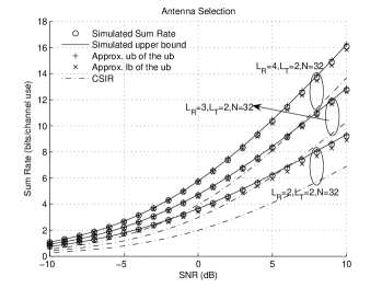
Figure 1: Sum Rate for Antenna Selection.

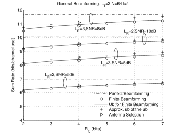
Figure 2: Sum Rate for General Beamforming.

V Conclusion

This paper proposes a strategy where users are controlled jointly. The effect of user choice is analyzed by extreme order statistics and the effect of beamforming is quantified by the distortion rate function in the composite Grassmann manifold. By characterizing the distortion rate function on the composite Grassmann manifold and calculating the logdet function of a random composite Grassmann matrix, a good sum rate approximation is derived.

References

• [1] K.Β K. Mukkavilli, A.Β Sabharwal, E.Β Erkip, and B.Β Aazhang, β€œOn beamforming with finite rate feedback in multiple-antenna systems,” IEEE Trans. Info. Theory, vol.Β 49, no.Β 10, pp. 2562–2579, 2003.
• [2] D.Β J. Love, J.Β Heath, R.Β W., and T.Β Strohmer, β€œGrassmannian beamforming for multiple-input multiple-output wireless systems,” IEEE Trans. Info. Theory, vol.Β 49, no.Β 10, pp. 2735–2747, 2003.
• [3] W.Β Santipach, Y.Β Sun, and M.Β L. Honig, β€œBenefits of limited feedback for wireless channels,” in Proc. Allerton Conf. on Commun., Control, and Computing, 2003.
• [4] J.Β C. Roh and B.Β D. Rao, β€œMIMO spatial multiplexing systems with limited feedback,” in Proc. IEEE International Conference on Communications (ICC), 2005.
• [5] D.Β Love and J.Β Heath, R.W., β€œLimited feedback unitary precoding for spatial multiplexing systems,” IEEE Trans. Info. Theory, to appear.
• [6] B.Β Mondal, R.Β W.Β H. Jr., and L.Β W. Hanlen, β€œQuantization on the Grassmann manifold: Applications to precoded MIMO wireless systems,” in Proc. IEEE International Conference on Acoustics, Speech, and Signal Processing (ICASSP), 2005, pp. 1025–1028.
• [7] W.Β Dai, Y.Β Liu, B.Β Rider, and V.Β K.Β N. Lau, β€œOn the information rate of MIMO systems with finite rate channel state feedback and power on/off strategy,” in Proc. IEEE International Symposium on Information Theory (ISIT), 2005.
• [8] W.Β Dai, Y.Β Liu, and B.Β Rider, β€œQuantization bounds on Grassmann manifolds and the application to MIMO systems,” in IEEE Global Telecommunications Conference (GLOBECOM), accepted, 2005.
• [9] D.Β Tse and S.Β Hanly, β€œMultiaccess fading channels. I. Polymatroid structure, optimalresource allocation and throughput capacities,” IEEE Trans. Info. Theory, vol.Β 44, no.Β 7, pp. 2796–2815, 1998.
• [10] V.Β Lau, L.Β Youjian, and T.Β A. Chen, β€œCapacity of memoryless channels and block-fading channels with designable cardinality-constrained channel state feedback,” IEEE Trans. Info. Theory, vol.Β 50, no.Β 9, pp. 2038–2049, 2004.
• [11] J.Β H. Conway, R.Β H. Hardin, and N.Β J.Β A. Sloane, β€œPacking lines, planes, etc., packing in grassmannian spaces,” Exper. Math., vol.Β 5, pp. 139–159, 1996.
• [12] R.Β J. Muirhead, Aspects of multivariate statistical theory.Β Β Β New York: John Wiley and Sons, 1982.
• [13] W.Β Dai, Y.Β Liu, V.Β K.Β N. Lau, and B.Β Rider, β€œOn the information rate of MIMO systems with finite rate channel state feedback using power on/off strategy,” IEEE Trans. Commun., submitted.
• [14] A.Β T. James, β€œNormal multivariate analysis and the orthogonal group,” Ann. Math. Statist., vol.Β 25, no.Β 1, pp. 40 – 75, 1954.