Variance Reduction for Particle Filters of Systems with Time Scale Separation

Abstract

We present a particle filter construction for a system that exhibits time scale separation. The separation of time scales allows two simplifications that we exploit: i) the use of the averaging principle for the dimensional reduction of the dynamics for each particle during the prediction step and ii) the factorization of the transition probability for the Rao-Blackwellization of the update step. The resulting particle filter is faster and has smaller variance than the particle filter based on the original system. The method is tested on a multiscale stochastic differential equation and on a multiscale pure jump diffusion motivated by chemical reactions.

I Introduction

The field of dimensional reduction has seen a flourishing in the last decade (see e.g. the reviews in [1, 2]), mainly due to i) the realization that many systems of physical interest are more complex than one can handle even with the largest available computers and ii) the fact that for many complex systems the quantities of interest are coarse-scale features. Once a reduced model is constructed, it can be used in conjunction with filtering algorithms, like particle filters [3], to incorporate information from real-time measurements. If the system under consideration exhibits time scale separation, the construction of a reduced model and subsequently of a particle filter, is also simplified. In this work we present a particle filter which exploits this simplification to create a particle filter that is more efficient than the particle filter of the original (large dimensional) system. The particle filter we construct is proved to converge to the analytical filter of the original system.

A strategy for reducing the number of unknowns in an application of a filter for nonlinear dynamical systems is proposed in [4]. In that work the authors assumed that the dynamics are strongly locally contractive in some directions which are found adaptively. Here we make an alternative assumption. We instead assume that the system exhibits a time scale separation. By this we mean that certain components or modes of the system tend to move very slowly in comparison with the rest of the modes. In particular we are interested in approximating conditional expectations the form

$$\mathbf{E}\left[f\left(X_{s_{k}}\right)|\left\{Z_{1},\dots,Z_{k}\right\}\right]$$

where $Z_{k}$ are noisy observations of some multiscale Markov process $X_{t}$ at discrete times $s_{1},\dots,s_{N}.$ For a very general definition of a multiscale Markov process see [5, 6] and [7]. We will illustrate the method presented below for the particular case that $X_{t}$ is the solution to a stochastic differential equations with time scale separation (see equation (III.1)). The basic idea, however, can be applied to filtering problems for a variety of multiscale Markov process for which fast multiscale integration methods are available (see [8, 9, 10, 11, 12, 13, 14, 7] and the references therein). In section IV, our filtering method is applied first to the reconstruction of the trajectory of a multiscale stochastic differential equation and second to the reconstruction of a trajectory of a pure jump Markov process motivated by chemical reactions that takes place on vastly different time scales.

Loosely speaking, recursive estimation of conditional expectations of the form above can be accomplished in two steps. First, in the prediction step, the system is evolved according to its evolution law. Second, in the update step, the resulting samples of the system are weighted by the likelihood of the next observation given the sample. We describe the filtering problem in more detail in the next section. The separation of time scales facilitates the construction of an efficient particle filter in two ways: i) it allows for fast evolution of the system in the prediction step and ii) it allows the integration of the observation weights over the fast modes of the system during the update step. Step ii) amounts to a Rao-Blackwellization of a standard particle filter estimator.

Multiscale phenomena have been observed in wide ranging areas of research. For example, empirical evidence from a study of exchange rate dynamics in [15], suggests the use of stochastic volatility models with both fast and slow time scales. Other examples of systems with scale separation include chemical reaction systems where there can exist a difference of several orders of magnitude among the different reaction rates (see [12, 13, 16, 17, 18]). Similar problems exist in material science (see [19]) and molecular dynamics simulations (see [20]) where one is interested in large scale features of the system but this behavior depends critically on the small (and fast) scale motion. An even more challenging problem is that of weather prediction and how to assimilate (through filtering) the vast amount of measurements collected daily around the globe. The weather system exhibits an extremely large range of active scales not necessarily with clear time scale separation (see [21, 22]). A projection formalism framework, for the construction of reduced models of large systems with or without time scale separation, has been presented by Chorin and co-workers (see [23]).

The main difficulty presented by multiscale phenomena is that they are extremely costly to integrate. The vast majority of computational time is spent evolving the fast components of the system while one may be primarily interested in slow scale characteristics. This implies that the prediction step in any filtering method which does not take directly into account the multiscale structure of the problem will become prohibitively costly as the time scale separation increases. As described in detail below, our method addresses this issue through its incorporation of the multiscale integration scheme.

A second issue, common to importance sampling techniques for high dimensional problems, is controlling the variance of the resulting estimator. To address this in the context of particle filtering, many authors have suggested the use of some form of Rao-Blackwellization (see [24, 25, 26, 27, 28, 29] for example). The distribution of the underlying Markov process given current and past observations can always be factored into a posterior marginal distribution for some set of (in our case slow) variables and a posterior conditional distribution for the remaining (in our case fast) variables given the first set of variables. Rao-Blackwellization requires that expectations with respect to the resulting posterior conditional distribution can be carried out exactly. In the case that the posterior conditional distribution can be sampled, the Rao-Blackwellization procedure can be approximated by Monte Carlo averaging over these samples. As discussed in detail later, the separation of scales assumption made in this paper allows an approximate factorization of the posterior distribution in which samples from the posterior conditional distribution can be easily and efficiently generated. While our assumption on the system clearly restricts the class of possible applications, another advantage of our setup is that the posterior conditional distribution of the unresolved variables is allowed to be quite general (for example very non-Gaussian).

A method closely related to the one presented here was recently proposed in [30]. There is, however, an important difference. In [30] it is assumed that the observations and the objective function ($f$ in the conditional expectation above) depend directly only on the slow modes in the system. Here we allow for general observations and general objective functions. This fact is central to the utility of our algorithm. The method proposed here is designed to not only improve the efficiency of the prediction step of a particle filter, but also to reduce the number of particles required to achieve a given accuracy. In fact, in some problems with a moderate time scale separation, one may not observe any gain in efficiency in the prediction step, while the reduction in variance may be significant. It should also be noted that analytical results for continuous time multiscale filtering problems have been obtained by Kushner in [31].

The paper is organized as follows. Section II recalls the well known particle filter construction for a general Markov process which is observed with noise at a discrete set of instants. Section III presents our particle filter construction in the particular case of a multiscale stochastic differential equation. Section III-A discusses how the presence of a separation of time scales can lead to a construction of a reduced model for the slow components of the system and how it allows the Rao-Blackwellization of the filtering step. It also includes a particle filter construction which is based on the assumption that the reduced model can be constructed analytically and the Rao-Blackwellization of the filtering step can be performed analytically. Section III-B contains the main algorithm, which approximates the particle filter presented in Section III-A when the necessary calculations cannot be performed analytically. Section IV-A contains numerical results for a system of stochastic differential equations. Section IV-B contains numerical results for a pure jump type Markov process motivated by multiscale chemical reactions. Finally, Section V contains a discussion of the algorithm and of the results.

II The filtering problem and particle filters

We start by formulating the filtering problem. Assume that $X_{t}$ is a $d$-dimensional Markov process with transition probability $Q_{\Delta s}(x,dx^{\prime})$ where $Q_{0}(dx)$ is a known distribution on $\mathbb{R}^{d}$. We assume for notational convenience, that the process is autonomous. The process $X_{t}$ is usually called the hidden signal. Assume, also, that we have noisy discrete observations at $N$ regularly spaced times of length $\Delta s=s_{k}-s_{k-1}$ for $k=1,\ldots,N$ where $s_{0}=0$ and $s_{k}$ the time of the $i$-th observation. The observations satisfy,

$$Z_{k}=G(X_{s_{k}},\chi_{k}),\quad k=1,\ldots,N$$

where the $\chi_{k}$ are i.i.d random variables, independent of $X_{t}$, and for all $x$ the variable $Z=G(x,\chi)$ admits a density $z\to g(x,z)$ which is known. Let $1:k$ denote the sequence $\left\{1,\ldots,k\right\}$ for $k=1,\ldots,N$. The filtering problem consists of computing the conditional expectations

$$\Pi_{k}f=\mathbf{E}\left[f(X_{s_{k}})|Z_{1:k}\right]\;\text{for}\;k=1,\ldots,N,$$

where $f$ belongs to some reasonable family of functions. The quantities $\Pi_{k}f$ constitute the filter (called the analytical filter).

The conditional expectation $\Pi_{k}f$ can be written as

$$\Pi_{k}f=\frac{\int Q_{0}(dx_{0})Q_{\Delta s}(x_{0},dx_{s_{1}})g(x_{s_{1}},z_{1})}{\int Q_{0}(dx_{0})Q_{\Delta s}(x_{0},dx_{s_{1}})g(x_{s_{1}},z_{1})}\\ \cdots\frac{Q_{\Delta s}(x_{s_{k-1}},dx_{s_{k}})g(x_{s_{k}},z_{k})f(x_{s_{k}})}{Q_{\Delta s}(x_{s_{k-1}},dx_{s_{k}})g(x_{s_{k}},z_{k})},$$ (II.1)

where $\int$ stands for integration over the variables $x_{s_{0}},x_{s_{1}},\dots,x_{s_{k}}.$ Let $H_{k}$ be the kernels,

$$H_{k}f\,(x_{s_{k-1}},z_{k})=\int Q_{\Delta s}(x_{s_{k-1}},dx_{s_{k}})\\ \times g(x_{s_{k}},z_{k})\ f(x_{s_{k}})\ dx_{s_{k}}.$$ (II.2)

The filter (II.1) can be written recursively as

$$\Pi_{0}f=\int f(x)\ Q_{0}(dx),\quad\Pi_{k}f=\frac{\Pi_{k-1}H_{k}\,f}{\Pi_{k-1}H_{k}\,1}.$$ (II.3)

Usually, the integrals in (II.3) cannot be computed analytically. A particle filter [32, 3] is an approximation to the analytical filter (II.3). In its simplest form, a particle filter consists of the following steps:

Algorithm II.1

Standard particle filter.

1. Sample $n$ i.i.d. vectors (particles) $X_{0}^{j},\;j=1,\ldots,n$ from $Q_{0}(dx).$ Set $k=1.$

2. For $j=1,\ldots,n$ evolve $X_{s_{k-1}}^{j}$ according to $Q_{\Delta s}(X_{s_{k-1}}^{j},dx^{\prime})$ to get ${X^{\prime}}_{s_{k}}^{j}$.

3. Calculate

   $$\begin{split}W^{n}_{k}\,f&=\frac{1}{n}\sum_{j=1}^{n}f({X^{\prime}}_{s_{k}}^{j})\,g({X^{\prime}}_{s_{k}}^{j},z_{k}),\\ W^{n}_{k}\,1&=\frac{1}{n}\sum_{j=1}^{n}\,g({X^{\prime}}_{s_{k}}^{j},z_{k}).\end{split}$$

4. Define the probability measure $\Psi^{n}_{k}$ on $\mathbb{R}^{d}$ with density

   $$\Psi^{n}_{k}(dx)=\frac{1}{n\,W^{n}_{k}\,1}\sum_{j=1}^{n}\ g({X^{\prime}}_{s_{k}}^{j},z_{k})\ \delta_{{X^{\prime}}_{s_{k}}^{j}}(dx).$$

5. If $k<N$: Set $k\rightarrow k+1.$ Sample $n$ i.i.d. variables ${X}_{s_{k}}^{j},\;j=1,\ldots,n$ from $\Psi^{n}_{k}$, and go to Step 2.

We stop at the end of iteration $N$, and our approximation of $\Pi_{k}\,f$ is,

$$\Psi_{k}^{n}\,f=\frac{W_{k}^{n}\,f}{W_{k}^{n}\,1}=\mathbf{E}_{\Psi_{k}^{n}}f$$

III Filtering for systems with time scale separation

III-A Scale separation and Rao-Blackwellization

Many problems in the natural sciences give rise to systems with time scale separation. These systems represent a challenge for numerical simulations. For example in molecular dynamics simulations femtoseconds timesteps are required to integrate the fastest atomic motions, while the object of interest is of orders of microseconds or longer. In the past four decades systems with scale separation have been the focus of extensive research within the framework of the averaging principle. The separation of scales is utilized to derive an effective model for the slow components of the system. While the averaging principle and its resulting effective dynamics provide a substantial simplification of the original system it is often impossible or impractical to obtain the reduced equations in closed form. This has motivated the development of algorithms such as multiscale integration methods described in the next section.

To make the presentation more concrete we will describe the situation for a $d$-dimensional systems of stochastic differential equations with multiple time scales (see [33] Chapter 7). As mentioned in the introduction, the ideas that we will discuss can be applied to filtering problems for any multiscale Markov process for which multiscale integration methods are available.

Let $(X^{\epsilon}_{t},Y^{\epsilon}_{t})$ be a solution of the system

$$dX^{\epsilon}_{t} =a(X^{\epsilon}_{t},Y^{\epsilon}_{t})\,dt+b(X^{\epsilon}_{t})\,dU_{t}, X^{\epsilon}_{0} =x_{0}$$ (III.1a)

$$dY^{\epsilon}_{t} =\frac{1}{\epsilon}\alpha(X^{\epsilon}_{t},Y^{\epsilon}_{t})\,dt+\frac{1}{\sqrt{\epsilon}}\beta(X^{\epsilon}_{t},Y^{\epsilon}_{t})\,dV_{t}, Y^{\epsilon}_{0} =y_{0}.$$ (III.1b)

where $U_{t}$ and $V_{t}$ are independent Brownian motions. The hidden variable $(X^{\epsilon}_{t},Y^{\epsilon}_{t})$ is a Markov process with transition probability $Q^{\epsilon}_{\Delta s}((x,y),(dx^{\prime},dy^{\prime}))$ on $\mathbb{R}^{d_{x}}\times\mathbb{R}^{d_{y}}$ (with $d_{x}+d_{y}=d$). The $X^{\epsilon}_{t}$ variables evolve on a $O(1)$ time scale (the macro time scale), and the $Y^{\epsilon}_{t}$ variables evolve on an $O(\epsilon)$ time scale (the micro time scale). As above, we have noisy discrete observations,

$$Z_{k}=G(X^{\epsilon}_{s_{k}},Y^{\epsilon}_{s_{k}},\chi_{k}),\;k=1,\ldots,N$$

where the $\chi_{k}$ are i.i.d variables, independent of $x,y$, and for all $x,y$ the variable $Z=G(x,y,\chi)$ admits a density $z\to g(x,y,z)$ which is known.

The standard approach to this filtering problem (see [34]) is to use an easily sampled approximation $Q^{\epsilon,\delta t}_{\Delta s}\left(\left(x,y\right),\left(dx^{\prime},dy^{\prime}\right)\right)$ of the transition probability $Q^{\epsilon}_{\Delta s}((x,y),(dx^{\prime},dy^{\prime}))$ where the discrete time step $\delta t$ is of scale comparable to $\epsilon.$ If one is interested in the evolution of the system over $O(1)$ time scales then one must evolve the system for $O(\frac{1}{\epsilon})$ steps, which can be very costly for systems with large scale separation. In addition to simulation issues inherent to multiscale phenomena, particle filters can suffer from all of the usual difficulties associated with importance sampling in large dimensional spaces. That is, in high dimensional systems, the variance of the particle filter estimator can be difficult to control.

In this section we show how the averaging principle and Rao-Blackwellization can be used to reduce the computational effort for each particle and the number of required particles. The method we discuss assumes that the Rao-Blackwellization and the construction of the dimensionally reduced model can be performed analytically. Unfortunately, this is rarely the case. In the next section, we show how the multiscale integration framework can be used to implement our approach when we are not able to perform the Rao-Blackwellization and the construction of the reduced model analytically.

Under appropriate assumptions (see [35, 5, 6, 33]), the averaging principle dictates that as $\epsilon\to 0$

$$X^{\epsilon}_{t}\overset{\mathscr{D}}{\longrightarrow}\;\bar{X}_{t}\;\text{for}\;t\in[0,T],$$

where $\bar{X}_{t}$ satisfies

$$d\bar{X}_{t}=\bar{a}(\bar{X}_{t})\,dt+b(\bar{X}_{t})\,dW_{t}.$$ (III.2)

The averaged coefficient $\bar{a}$ is given by

$$\bar{a}(x) =\int_{\mathbb{R}^{d_{y}}}a(x,y)\mu_{x}(dy)$$ (III.3)

where $\mu_{x}(dy)$ is the invariant measure induced by (III.1b) with the $x$ variables fixed.

The key consequence of the time scale separation is that, loosely speaking, for $\epsilon$ small enough and for $\Delta s\gg\epsilon,$ the transition density $Q^{\epsilon}_{\Delta s}\left((x,y),(dx^{\prime},dy^{\prime})\right)$ can be approximately factored as

$$Q^{\epsilon}_{\Delta s}\left((x,y),(dx^{\prime},dy^{\prime})\right)\approx\bar{Q}_{\Delta s}(x,dx^{\prime})\,\mu_{x^{\prime}}(dy)$$ (III.4)

where $\bar{Q}_{\Delta s}$ is the transition density for the averaged system, (III.2). The factorization (III.4) above is the central tool in the construction of the multiscale particle filter below and is not a feature limited to multiscale stochastic differential equations. The algorithms below apply to any problem for which this approximation holds and for which some means of sampling (or approximately sampling) $\bar{Q}_{\Delta s}(x,dx^{\prime})$ and $\mu_{x^{\prime}}(dy)$ are available. This is the case for both of the examples in Section IV.

The relation (III.4) suggests that an approximate particle filter can be constructed by defining the kernel,

$$\bar{H}_{k}f\,(x_{s_{k-1}},z_{k})=\int\bar{Q}_{\Delta s}(x_{s_{k-1}},dx_{s_{k}})\\ \times\mu_{x_{s_{k}}}(dy)\ g(x_{s_{k}},y,z_{k})\ f(x_{s_{k}},y).$$ (III.5)

The corresponding particle filter would proceed as follows,

Algorithm III.1

Standard particle filter corresponding to (III.5).

1. Sample $n$ i.i.d. vectors $(X_{0}^{j},Y_{0}^{j})\;j=1,\ldots,n$ from $Q_{0}(dx,dy)$ distribution. Set $k=1.$

2. For each $j,$ use (III.3) to evolve $X_{s_{k-1}}^{j}$ to ${X^{\prime}_{s_{k}}}^{j},$ i.e., sample from $\bar{Q}_{\Delta s}(X_{s_{k-1}}^{j},dx^{\prime}).$ For each sample ${X^{\prime}_{s_{k}}}^{j},$ generate an independent sample ${Y^{\prime}}^{j}$ from the measure $\mu_{{X^{\prime}_{s_{k}}}^{j}}.$

3. Calculate,

   $$\begin{split}W^{n}_{k}\,f&=\frac{1}{n}\sum_{j=1}^{n}f({X^{\prime}_{s_{k}}}^{j})\,g({X^{\prime}_{s_{k}}}^{j},{Y^{\prime}}^{j},z_{k})\\ W^{n}_{k}\,1&=\frac{1}{n}\sum_{j=1}^{n}g({X^{\prime}_{s_{k}}}^{j},{Y^{\prime}}^{j},z_{k}).\end{split}$$

4. Define the probability measure $\Psi^{n}_{k}$ on $\mathbb{R}^{d}$ with density

   $$\Psi^{n}_{k}(dx,dy)=\frac{1}{nW^{n}_{k}1}\\ \times\sum_{j=1}^{n}\ g({X^{\prime}_{s_{k}}}^{j},{Y^{\prime}}^{j},z_{k})\ \delta_{{X^{\prime}_{s_{k}}}^{j}}(dx)\ \delta_{{Y^{\prime}}^{j}}(dy).$$

5. If $k<N$: Set $k\rightarrow k+1.$ Sample $n$ i.i.d. variables $X_{s_{k}}^{j},\;j=1,\ldots,n$ from $\Psi^{n}_{k}$, and go to Step 2.

We stop at the end of iteration $N$, and our approximation of $\Pi_{k}\,f$ is,

$$\Psi_{k}^{n}\,f=\frac{W_{k}^{n}\,f}{W_{k}^{n}\,1}=\mathbf{E}_{\Psi_{k}^{n}}f$$

There is no reason to hope that this algorithm should provide any variance reduction. Indeed, in the ideal case that expression (III.4) is an equality, the variance of the particle filter would be identical to the variance of the standard particle filter II.3.

However, knowledge of $\mu_{x_{s_{k}}}(dy)$ allows one to integrate out $y$ in expression (III.5) and write this same kernel in another form,

$$\bar{H}_{k}f\,(x_{s_{k-1}},z_{k})=\int\bar{Q}_{\Delta s}(x_{s_{k-1}},dx_{s_{k}})\\ \times\int\mu_{x_{s_{k}}}(dy)\ g(x_{s_{k}},y,z_{k})\ f(x_{s_{k}},y).$$ (III.6)

This suggests a different filtering algorithm:

Algorithm III.2

Rao-Blackwellized particle filter corresponding to (III.6).

1. Sample $n$ i.i.d. vectors $(X_{0}^{j},Y_{0}^{j})\;j=1,\ldots,n$ from $Q_{0}(dx,dy)$ distribution. Set $k=1.$

2. For each $j,$ use (III.3) to evolve $X_{s_{k-1}}^{j}$ to ${X^{\prime}_{s_{k}}}^{j},$ i.e., sample from $\bar{Q}_{\Delta s}(X_{s_{k-1}}^{j},dx^{\prime}).$

3. Calculate the following quantities:

   1. $$\left[\mu fg\right]({X^{\prime}_{s_{k}}}^{j}) =\int f({X^{\prime}_{s_{k}}}^{j},y)\,$$

      $$\hskip 14.22636pt\times g({X^{\prime}_{s_{k}}}^{j},y,z_{k})\mu_{{X^{\prime}_{s_{k}}}^{j}}(dy)$$

      $$\left[\mu g\right]({X^{\prime}_{s_{k}}}^{j}) =\int g({X^{\prime}_{s_{k}}}^{j},y,z_{k})\,\mu_{{X^{\prime}_{s_{k}}}^{j}}(dy).$$

   2. $$\begin{split}W^{n}_{k}\,f&=\frac{1}{n}\sum_{j=1}^{n}\left[\mu fg\right]({X^{\prime}_{s_{k}}}^{j})\\ W^{n}_{k}\,1&=\frac{1}{n}\sum_{j=1}^{n}\left[\mu g\right]({X^{\prime}_{s_{k}}}^{j}).\end{split}$$

4. Define the probability measure $\Psi^{n}_{k}$ on $\mathbb{R}^{d}$ with density

   $$\bar{\Psi}^{n}_{k}(dx,dy)=\frac{1}{n\,W^{n}_{k}\,1}\\ \times\sum_{j=1}^{n}\ g({X^{\prime}_{s_{k}}}^{j},y,z_{k})\ \delta_{{X^{\prime}_{s_{k}}}^{j}}(dx)\ \mu_{{X^{\prime}_{s_{k}}}^{j}}(dy).$$

5. If $k<N$: Set $k\rightarrow k+1.$ Sample $n$ i.i.d. variables $X_{s_{k}}^{j},\;j=1,\ldots,n$ from $\bar{\Psi}^{n}_{k}$, and go to Step 2.

We stop at the end of iteration $N$, and our approximation of $\Pi_{k}\,f$ is,

$$\bar{\Psi}_{k}^{n}\,f=\frac{W_{k}^{n}\,f}{W_{k}^{n}\,1}=\mathbf{E}_{\bar{\Psi}_{k}^{n}}f$$ (III.7)

Since the $y$ components of the resampled particles after Step 4 are not used in Step 2, we can, in practice, resample from the marginal density

$$\bar{\Psi}^{n}_{k}(dx)=\frac{1}{n\,W^{n}_{k}\,1}\sum_{j=1}^{n}\ \left[\mu g\right]\left({X^{\prime}_{s_{k}}}^{j}\right)\ \delta_{{X^{\prime}_{s_{k}}}^{j}}(dx).$$ (III.8)

In order to illustrate the variance reduction aspects of algorithm III.2 we will consider the asymptotic variance of a pair of related but much simpler estimators. Define the conditional expectations $\bar{\Pi}_{k}$ recursively by,

$$\bar{\Pi}_{0}f=\int f(x)\ Q_{0}(dx),\quad\bar{\Pi}_{k}f=\frac{\bar{\Pi}_{k-1}\bar{H}_{k}\,f}{\bar{\Pi}_{k-1}\bar{H}_{k}\,1}.$$

Let

$$I^{n}_{k}f=\frac{\frac{1}{n}\sum_{j=1}^{n}f(X^{j}_{k},Y^{j}_{k})\,g(X^{j}_{k},Y^{j}_{k},z_{k})}{\frac{1}{n}\sum_{j=1}^{n}g(X^{j}_{k},Y^{j}_{k},z_{k})}$$

and

$$\bar{I}^{n}_{k}f=\frac{\frac{1}{n}\sum_{j=1}^{n}\left[\mu fg\right](X^{j}_{k})}{\frac{1}{n}\sum_{j=1}^{n}\left[g\right](X^{j}_{k})}$$

where $(X^{j}_{k},Y^{j}_{k})$ are $i.i.d.$ samples from the measure $\Pi_{k-1}\bar{Q}_{\Delta s}\mu$ Notice that the only difference between $I^{n}_{k}f$ and $\Psi^{n}_{k}f$ described in Algorithm (III.5) is that the samples $(X^{j}_{k},Y^{j}_{k})$ are independently drawn from $\bar{\Pi}_{k-1}\bar{Q}_{\Delta s}\mu$ instead of its particle approximation $\Psi^{n}_{k-1}\bar{Q}_{\Delta s}\mu.$ A corresponding relationship holds between $\bar{I}^{n}_{k}f$ and $\bar{\Psi}^{n}_{k}f.$

The estimators $I^{n}_{k}f$ and $\bar{I}^{n}_{k}f$ satisfy Central Limit Theorems, i.e.

$$\sqrt{n}\left(I^{n}_{k}f-\bar{\Pi}_{k}f\right)\xrightarrow{\mathscr{D}}\mathcal{N}\left(0,\sigma^{2}\right)$$ (III.9)

and

$$\sqrt{n}\left(\bar{I}^{n}_{k}f-\bar{\Pi}_{k}f\right)\xrightarrow{\mathscr{D}}\mathcal{N}\left(0,\bar{\sigma}^{2}\right).$$ (III.10)

An application of the delta method (see [36]) yields that

$$\sigma^{2}=\bar{\Pi}_{k-1}\bar{Q}_{\Delta s}\mu\\ \left[\left(f(X,Y)-\bar{\Pi}_{k}f\right)^{2}\left(\frac{g(X,Y)}{\bar{\Pi}_{k-1}\bar{H}_{k}1}\right)^{2}\right]$$

and

$$\bar{\sigma}^{2}=\bar{\Pi}_{k-1}\bar{Q}_{\Delta s}\left[\left(\frac{\left[\mu fg\right]({X})}{\left[\mu g\right](X)}-\bar{\Pi}_{k}f\right)^{2}\left(\frac{\left[\mu g\right](X)}{\bar{\Pi}_{k-1}\bar{H}_{k}1}\right)^{2}\right].$$

$\bar{\sigma}^{2}$ can be rewritten as

$$\bar{\Pi}_{k-1}\bar{Q}_{\Delta s}\left[\left[\mu\left(\frac{fg-g\bar{\Pi}_{k}f}{\bar{\Pi}_{k-1}\bar{H}_{k}1}\right)\right]^{2}(X)\right].$$

Therefore, by Jensen’s inequality, we have that

$$\bar{\sigma}^{2}\leq\bar{\Pi}_{k-1}\bar{Q}_{\Delta s}\left[\mu\left(\frac{fg-g\bar{\Pi}_{k}f}{\bar{\Pi}_{k-1}\bar{H}_{k}1}\right)^{2}\right]=\sigma^{2}.$$

It is important to note that the variance reduction offered by Algorithm III.2 does not require any Gaussian or degenerate measure approximations. The main assumptions are that the system have a multiscale structure and that one can sample from $\bar{Q}_{\Delta s}(x,dx^{\prime})$ and evaluate averages with respect to the ergodic measure $\mu_{x}$ (which we assume exists). In many cases, for example those in Section IV, the first assumption can be easily verified. For most general systems, $\bar{Q}_{\Delta s}(x,dx^{\prime})$ is not available in closed form. In practice, we must replace $\bar{Q}_{\Delta s}$ by some approximation. For example in the case of $\bar{x}_{t}$ above we can use the transition probability kernel for the Euler-Maruyama scheme with step size $\Delta t,$ $\bar{Q}^{\Delta t}_{\Delta s}.$ Of course to apply the Euler approximation to (III.2) we must be able to exactly evaluate averages with respect to $\mu_{x}.$ The removal of this assumption will be addressed in the next section.

III-B Implementation of the multiscale integration for the reduced particle filter

In the particle filter construction of the previous section we used the fact that we can average over the invariant measure induced by the fast variables. This is usually impossible since the invariant measure is unknown or because integration cannot be performed analytically. We will demonstrate that this problem can be overcome by using multiscale integration schemes (see [8, 9, 10, 11, 12, 13, 14]). In the following description we will be discussing specifically the multiscale integration schemes of the form analyzed in [10] and [11]. The system studied in section IV-B is a pure jump Markov process and therefore requires a different multiscale integration scheme (see [12, 13]). Let $\Delta t$ be a fixed time step, and $X_{k,l}$ be the numerical approximation to the coarse variable, $\bar{X}$ from the previous section, at time $t_{k,l}=s_{k}+l\Delta t$ (recall $s_{k}$ is the $k$-th observation time). Assume for simplicity that $L=\frac{\Delta s}{\Delta t}$ is an integer. Inspired by the limiting equation (III.2), $X_{k,l}$ is evolved in time by an Euler-Maruyama step,

$$X_{k,l+1}=X_{k,l}+A(X_{k,l})\,\Delta t+b(X_{k,l})\,\Delta W_{t_{k,l}}$$ (III.11)

for $l=0,\dots,L-1,$ where $\Delta W_{t_{k,l}}$ are Brownian displacements over a time interval $\Delta t$. We refer to (III.11) as the macro-solver, or macro integrator, and we denote its transition probability by $\bar{Q}^{\Delta t,\delta t,M}_{\Delta s}(x,dx^{\prime}).$ Notice that with this notation $X_{k,0}=X_{k-1,L}.$

The function $A(x)$ approximates $\bar{a}(x),$ introduced in the previous section, which is the average of $a$ over an ergodic measure. The ergodic property implies that instead of ensemble averaging we can use time averaging over trajectories of the rapid variables with fixed $x$. Since, by assumption, this average cannot be performed analytically, it is approximated by an empirical average over short runs of the fast dynamics. These “short runs” are over time intervals that are sufficiently long for empirical averages to be close to their limiting ensemble averages, yet sufficiently short for the entire procedure to be efficient compared to the direct solution of the coupled system.

Thus, given the coarse variable at the ${k,l}$-th time step, $X_{k,l}$, we take some initial value for the fast component $Y_{k,l,0}$, and solve (III.1b) numerically with step size $\delta t$ and $x=X_{k,l}$ fixed. We denote the discrete variables associated with the fast dynamics at the ${k,l}$-th coarse step by $Y_{k,l,m}$, $m=0,1,\dots,M.$ The numerical solver used to generate the sequence $Y_{k,l,m}$ is called the micro-solver, or micro-integrator. The simplest choice is again the Euler-Maruyama scheme,

$$Y_{k,l,m+1}=Y_{k,l,m}+\frac{1}{\epsilon}\alpha(X_{k,l},Y_{k,l,m})\,\delta t\\ +\frac{1}{\sqrt{\epsilon}}\beta(X_{k,l},Y_{k,l,m})\Delta V_{k,l,m},$$ (III.12)

where $\Delta V_{k,l,m}$ are Brownian displacements over a time interval $\delta t$. In this equation $X_{k,l}$ is a parameter in $Y_{k,l,m}$ though this will not be explicitly written. Since we assume that the dynamics of the $y$ variables is ergodic, we may choose $Y_{k,l,0}=Y_{k,l-1,m}$ for all $k$ and $l$. For convenience however, we will set $Y_{k,l,0}=0.$ As for the $X$ variables, our notation implies $Y_{k,0,m}=Y_{k-1,L,m}$ for all $m.$

The existence, under appropriate assumptions, of an invariant measure, $\mu_{x}^{\delta t},$ of the numerical scheme (III.12), follows from results in [37, 38]. The measure $\mu_{x}^{\delta t}$ is an approximation to $\mu_{x}.$ This suggests estimating the function $\bar{a}$ by

$$A(X_{k,l})=\frac{1}{M}\sum_{m=1}^{M}a(X_{k,l},Y_{k,l,m}).$$ (III.13)

Since we will frequently encounter this form of trajectory averaging in the sequel, we define the symbol

$$\left[\mathcal{S}^{M}h\right](y_{1},\dots,y_{m})=\frac{1}{M}\sum_{m=1}^{M}h(y_{m}),$$

where $h$ is some function defined on $\mathbb{R}^{d_{y}}.$ We will henceforth omit from our notation, the dependence of $\mathcal{S}^{M}h$ on the variables $(y_{1},\dots,y_{m}).$ Equations (III.11), (III.12), and (III.13) define the multiscale integration scheme. We note here that, in fact, since for our filtering application of the multiscale integration scheme we are interested in reproducing the distribution of the process (III.1) and not actual trajectories, we can replace the average in (III.13) by evaluation at the single point $Y_{k,l,M}.$ Since expression (III.13) is only marginally more expensive and corresponds more naturally to the method of averaging, we will not bother with this simplification.

Suppose that the joint distribution of $Y_{k,l,m}$ given that $X_{k,l}=x$ and $Y_{k,l,0}=0$ is $\widetilde{Q}^{\delta t,M}_{x}(dy_{1},\dots,dy_{M}).$ We can define the measure $\mu^{M}_{x}$ by,

$$\mu_{x}^{M}h=\widetilde{Q}^{\delta t,M}\mathcal{S}^{M}h(y_{m})=\frac{1}{M}\sum_{m=1}^{M}\mathbf{E}_{x}h(Y_{k,l,m}).$$

where the subscript $x$ on the expectation emphasizes the dependence of the random variables $Y_{k,l,m}$ on the parameter $x.$

By using trajectory averages over the fast dynamics to approximate integrals over $\mu_{x}$ of the observation density as well as the coefficient $\bar{a}$ we can define a particle filter which approximates the Rao-Blackwellization step of the previous section. The following kernel is an approximation of expression (III.6),

$$\bar{H}_{k}^{\Delta t,\delta t,M}f\,(x_{s_{k-1}},z_{k})=\int\bar{Q}_{\Delta s}^{\Delta t,\delta t,M}(x_{s_{k-1}},dx_{s_{k}})\\ \times\mu_{x_{s_{k}}}^{M}(dy)\,f(x_{s_{k}},y)\,g(x_{s_{k}},y,z_{k}).$$ (III.14)

The next particle filter, defined in the following algorithm, corresponds to (III.14) and differs from Algorithm III.2 in that we evolve the particles according to $\bar{Q}^{\Delta t,\delta t,M}_{\Delta s}$ instead of $\bar{Q}_{\Delta s}$ and, in the update Step, instead averaging over the measure $\mu_{x}$ we average over a trajectory of $Y^{j}_{k,l,m}.$

Algorithm III.3

Multiscale particle filter

1. Sample $n$ i.i.d. vectors $X_{0}^{j}\;j=1,\ldots,n$ from $Q_{0}(dx,dy).$ Set $k=1.$

2. For each $j=1,\ldots,n$ evolve $X^{\prime}_{k-1,0}=X^{j}_{k-1}$ according to Equations III.11, III.12, and III.13 to generate samples ${X^{\prime}_{k}}^{j}={X^{\prime}}_{k-1,L}^{j}$, i.e. sample from $\bar{Q}^{\Delta t,\delta t,M}_{\triangle s}(X_{k-1}^{j},dx^{\prime}).$ We use ${Y^{\prime}}^{j}_{k-1,l,m}$ to denote the fast variables evolved according to Eq. (III.12) with parameter ${X^{\prime}}^{j}_{k-1,l}.$ To initialize the ${Y^{\prime}}^{j}$ variables at each time Step of Eq. (III.11) we choose, ${Y^{\prime}}^{j}_{k,l,0}=0.$

3. For each $j=1,\ldots,n:$

   1. Evolve ${Y^{\prime}}_{k,0,0}^{j}=0$ according to (III.12) with parameter ${X^{\prime}_{k}}^{j}$ to get ${Y^{\prime}}_{k,0,m}^{j}\;\text{where}\;1\leq m\leq M$.

   2. Calculate

      $$\left[\mathcal{S}^{M}fg\right]({X^{\prime}_{k}}^{j}) =\frac{1}{M}\sum_{m=1}^{M}f({X^{\prime}_{k}}^{j},Y_{k,0,m}^{j})$$

      $$\hskip 28.45274pt\times g({X^{\prime}}_{k}^{j},Y_{k,0,m}^{j},z_{k})$$

      $$\left[\mathcal{S}^{M}g\right]({X^{\prime}_{k}}^{j}) =\frac{1}{M}\sum_{m=1}^{M}\,g({X^{\prime}_{k}}^{j},Y_{k,0,m}^{j},z_{k}).$$

   3. Calculate

      $$\begin{split}W^{n}_{k}\,f&=\frac{1}{n}\sum_{j=1}^{n}\left[\mathcal{S}^{M}fg\right]({X^{\prime}_{k}}^{j})\\ W^{n}_{k}\,1&=\frac{1}{n}\sum_{j=1}^{n}\left[\mathcal{S}^{M}g\right]({X^{\prime}_{k}}^{j}).\end{split}$$

4. Define the probability measure $\Psi^{n}_{k}$ on $\mathbb{R}^{d}$ with density

   $$\bar{\Psi}^{\Delta t,\delta t,M,n}_{k}(dx,dy)=\frac{1}{Mn\,W^{n}_{k}\,1}\\ \times\sum_{j=1}^{n}\sum_{m=1}^{M}\,g({X^{\prime}_{k}}^{j},Y_{k,0,m}^{j},z_{k})\,\delta_{{X^{\prime}_{k}}^{j}}(dx)\,\delta_{Y_{k,0,m}^{j}}(dy)$$

5. If $k<N$: Set $k\rightarrow k+1.$ Sample $n$ i.i.d. variables $X_{k}^{j}$, $\;j=1,\ldots,n$ from $\Psi^{n}_{k}$, and go to Step 2.

We stop at the end of iteration $N$, and our approximation of $\Pi_{k}\,f$ is,

$$\bar{\Psi}_{k}^{\Delta t,\delta t,M,n}\,f=\frac{W_{k}^{n}\,f}{W_{k}^{n}\,1}=\mathbf{E}_{\bar{\Psi}_{k}^{\Delta t,\delta t,M,n}}f$$

Since the $y$ components of the resampled particles after Step 4 are not used in Step 2, we can, in practice, resample from the marginal density

$$\bar{\Psi}^{\Delta t,\delta t,M,n}_{k}(dx)=\frac{1}{n\,W^{n}_{k}\,1}\sum_{j=1}^{n}\,\left[\mathcal{S}^{M}g\right]\left({X^{\prime}_{k}}^{j}\right)\,\delta_{{X^{\prime}_{k}}^{j}}(dx).$$ (III.15)

The two procedures give equivalent estimates and differ only in that the work required for the resampling Step using (III.15) will scale with $n$ instead of $nM$ (of course calculating the averaged weights requires $\mathcal{O}(nM)$ work). In practice to initialize ${Y^{\prime}}^{j}$ variables at each time Step of Eq. (III.11) we set, ${Y^{\prime}}^{j}_{k,l,0}={Y^{\prime}}^{j}_{k,l-1,m}.$ This choice results in faster equilibration of the $Y^{\prime}$ process.

While the details of the multiscale integration scheme do depend on the particular Markov process under study, algorithm III.3 can be applied in the same form to a wide variety of multiscale Markov processes (for example the system in section IV-B).

IV Numerical results

IV-A A stochastic differential equation

We present a simple numerical example which demonstrates the variance reduction obtained through our algorithm. Consider the system given by,

$$dX^{\epsilon}_{t} =\left(Y^{\epsilon}_{t}-(X^{\epsilon}_{t})^{3}\right)\,dt+dU_{t} X^{\epsilon}_{0} \sim\mathcal{N}(0,1)$$ (IV.1)

$$dY^{\epsilon}_{t} =\frac{2}{\epsilon}\left((X^{\epsilon}_{t})^{2}-(Y^{\epsilon}_{t})^{2}\right)Y^{\epsilon}_{t}\,dt+\frac{1}{\sqrt{\epsilon}}\,dV_{t} Y^{\epsilon}_{0} \sim\mathcal{N}(0,1).$$

The parameter $\epsilon$ in this example is set to $10^{-4}.$ A trajectory of the system is shown in Figure 1.

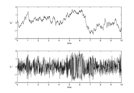
Figure 1: Trajectory of system (IV.1).

The ergodic measure of the fast dynamics for this system is known and has the bimodal density

$$\mu_{x}(y)=\frac{e^{-(x^{2}-y^{2})^{2}}}{\int e^{-(x^{2}-y^{2})^{2}}dy}.$$

A plot of $\mu_{x}$ for $x=1$ is shown in Figure 2.

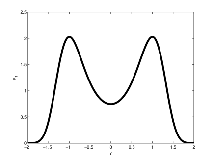
Figure 2: The density $\mu_{x}$ for $x=1.$

The observations are given by,

$$Z_{k}=Y^{\epsilon}_{k}+\chi_{k},$$

where $\chi$ are independent Gaussian random variables with mean 0 and standard deviation 0.1. In the experiment below we take as the realization of the observations, $z_{k},$ the trajectory shown in Figure 1 sampled at every one unit of time. We will compare the standard particle filtering algorithm with Algorithm III.3. Both methods are run with 1000 particles. System (IV.1) is discretized by the Euler-Maruyama method with time step $\delta t=10^{-6}.$ The multiscale integration scheme uses a time steps of size $\triangle t=10^{-2}$ to evolve the reduced system (III.11) and of size $\delta t$ in the microscopic system (III.12). With this choice of parameters Algorithm III.3 runs in about half of the time of the standard particle filter.

As in the definitions of the particle filters above, for any function $f$ define

$$W_{1}f\,(k)=\sum_{j=1}^{n}f({{X_{k}^{\epsilon}}^{\prime}}^{j},{{Y^{\epsilon}}^{\prime}}^{j})\,g({{X_{k}^{\epsilon}}^{\prime}}^{j},{{Y^{\epsilon}}^{\prime}}^{j},z_{k})$$

and

$$W_{2}f\,(k)=\\ \frac{1}{n10^{4}}\sum_{j=1}^{n}\sum_{m=1}^{10^{4}}f({X_{k}^{\prime}}^{j},Y_{k,0,m}^{j})\,g({X_{k}^{\prime}}^{j},Y_{k,0,m}^{j},z_{k}).$$

In Figure 3 we compare the pairs of estimators,

$$e^{1}_{x}(k)=\frac{W_{1}x\,(k)}{W_{1}1\,(k)},\ \ \ \ e^{1}_{y}(k)=\frac{W_{1}y\,(k)}{W_{1}1\,(k)}$$

and

$$e^{2}_{x}(k)=\frac{W_{2}x\,(k)}{W_{2}1\,(k)},\ \ \ \ e^{2}_{y}(k)=\frac{W_{2}y\,(k)}{W_{2}1\,(k)}$$

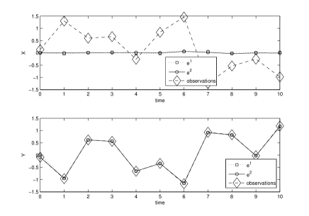
Figure 3: Trajectories of $e^{1}$ and $e^{2}.$

Notice that the poor quality of the reconstruction of $X^{\epsilon}_{t}$ is not due to an error. The symmetry of the observation model and of the $Y^{\epsilon}_{t}$ dynamics, implies that, in the limit $\epsilon\rightarrow 0,$ the true condition expectation of $X^{\epsilon}_{t},$ given any observations of $Y^{\epsilon}_{t}$ alone, will be identically zero. Therefore, both estimators appear to be accurate.

In order to compare the quality of the samples generated by the two methods we compute the effective sample sizes of the empirical measures produced by both methods,

$$ess_{1}(k)=\frac{1000}{1+C^{2}_{1}(k)}\quad\text{and}\quad ess_{2}(k)=\frac{1000}{1+C^{2}_{2}(k)}$$

where

$$C_{1}(k)=\frac{1}{W_{1}1\,(k)}\sqrt{\frac{1}{n}\sum_{j=1}^{n}\left(g({{X_{k}^{\epsilon}}^{\prime}}^{j},{{Y^{\epsilon}}^{\prime}}^{j},z_{k})-W_{1}1\,(k)\right)^{2}}$$

and

$$C_{2}(k)=\frac{1}{W_{2}1\,(k)}\sqrt{\frac{1}{n10^{4}}}\\ \times\sqrt{\sum_{j=1}^{n}\sum_{m=0}^{10^{4}}\left(g({X_{k}^{\prime}}^{j}_{6}(l),Y_{k,0,m}^{j},z_{k})-W_{2}1\,(k)\right)^{2}}.$$

The effective sample size is a common measure of the quality of a weighted empirical measure produced by an importance sampling scheme (see [39]). Very roughly, the effective sample size gives the number of independent samples from the target measure that would produce an unweighted empirical measure of equal quality. When all of the weights are equal (i.e. the samples are drawn from the target measure itself) the effective sample size is the total number of samples (in our case 1000).

The trajectories of $ess_{1}$ and $ess_{2}$ are plotted in Figure 4.

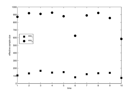
Figure 4: Trajectories of $ess_{1}$ and $ess_{2}.$

As can be seen in the plot, the effective sample sizes generated by Algorithm III.3 are nearly 10 times as large as those generated by the standard particle filter. This indicates that there is some improvement in the quality of the empirical measure generated by Algorithm III.3.

It is important to note while the cost of the two methods in this experiment are comparable, in the limit $\epsilon\rightarrow 0$ a discretization of the system (IV.1) would require smaller and smaller time steps. Thus the computational advantage for the multiscale particle filter would become extreme in this limit. The next example features a larger time scale separation and a correspondingly larger gain in efficiency due to multiscale integration.

IV-B A pure jump type Markov process

We now demonstrate our algorithm with a numerical example motivated by chemical reactions. The stochastic dynamical behavior of a well stirred mixture of $N$ molecular species that chemically interact through $M$ reaction channels is accurately described by the chemical master equation. The master equation is usually simulated using the Stochastic Simulation Algorithm of Gillespie [40]. In cellular systems where the small number of molecules of a few reactant species sometimes necessitates a stochastic description of the system’s temporal behavior, chemical reactions often take place on vastly different time scales. An exact stochastic simulation of such a system will necessarily spend most of its time simulating the more numerous fast reaction events.

For $N$ molecular species the state of the system $\mathbb{S}=\left(S_{1}(t),\ldots,S_{N}(t)\right)$ is the number of molecules of each species present at time $t$. The molecular populations $S_{i},i=1,\ldots,N$ are random variables. For each reaction channel $R_{j},j=1,\ldots,M$ we define the propensity function $a_{j}(\mathbb{S})$ and the state change vector $v_{j}$. The propensity function is such that $a_{j}(\mathbb{S})dt$ is the probability given $\mathbb{S}(t)=\mathbb{S}$ that one $R_{j}$ reaction will occur in the next infinitesimal time interval $\left[t,t+dt\right]$. The state change vector $v_{j}$ is the change in the number of $S_{i}$ molecules produced by one $R_{j}$ reaction.

The pathwise evolution law for the master equation is a jump type Markov process on the non negative $N$-dimensional integer lattice given by

$$\left(\begin{array}[]{c}dS_{1}\\ \vdots\\ dS_{N}\end{array}\right)=\left(\begin{array}[]{ccc}v_{1,1}&\ldots&v_{1,M}\\ \vdots&&\vdots\\ v_{N,1}&\ldots&v_{N,M}\end{array}\right)\\ \times\left(\begin{array}[]{c}dP_{1}(a_{1}(\mathbb{S}))\\ \vdots\\ dP_{M}(a_{M}(\mathbb{S}))\end{array}\right),$$ (IV.2)

where $P_{j}$ is a Poisson process with state dependent intensity parameter $a_{j}(\mathbb{S})$.

In our system we choose $N=6$ species and $M=5$ reaction channels. Variables $S_{1},\dots,S_{5}$ are the fast variables and $S_{6}$ is the slow variable. For the evolution of the fast variables we choose a simple fast biomolecular (reversible) reaction

$$S_{1}+S_{2} \to_{k_{1}}S_{3}$$

$$S_{3}+S_{6} \to_{k_{2}}S_{1}+S_{2}+S_{6},$$

and a fast (reversible) dimerization

$$S_{4}+S_{4} \to_{k_{3}}S_{5}$$

$$S_{5}+S_{6} \to_{k_{4}}S_{4}+S_{4}+S_{6}.$$

The propensity functions are given by

$$\begin{split}\left(\begin{array}[]{c}a_{1}(\mathbb{S})\\ a_{2}(\mathbb{S})\\ a_{3}(\mathbb{S})\\ a_{4}(\mathbb{S})\end{array}\right)&=\left(\begin{array}[]{c}k_{1}S_{1}S_{2}\\ k_{2}S_{3}S_{6}\\ k_{3}S_{4}(S_{4}-1)\\ k_{4}S_{5}S_{6}\end{array}\right)\end{split}$$

where the reaction rates $k_{1},\dots,k_{5}$ are specified below. We will use the shorthand

$$S_{f}=\left(S_{1},\dots,S_{5}\right).$$

For the slow variable $S_{6}$ we choose an external source (spontaneous creation)

$$S_{3}+S_{4}\to_{k_{5}}S_{3}+S_{4}+S_{6},$$

which is coupled to the fast variables through the slow reaction’s propensity function

$$a_{5}(\mathbb{S})=k_{5}S_{3}S_{4}.$$

The state change vectors for the system just described are given by the matrix,

$$\left(\begin{array}[]{ccc}v_{1,1}&\ldots&v_{1,5}\\ \vdots&&\vdots\\ v_{6,1}&\ldots&v_{6,5}\end{array}\right)=\left(\begin{array}[]{ccc}-1,\ 1,\ 0,\ 0,\ 0\\ -1,\ 1,\ 0,\ 0,\ 0\\ \ 1,-1,\ 0,\ 0,\ 0\\ \ 0,\ 0,-2,\ 2,\ 0\\ \ 0,\ 0,\ 1,-1,\ 0\\ \ 0,\ 0,\ 0,\ 0,\ 1\end{array}\right)$$

Finally the reaction constants vector is given by

$$\left(k_{1},\ldots,k_{5}\right)=\left(1000,1000,1000,1000,5\times 10^{-5}\right)$$

A trajectory of this system is plotted in Figure 5. One can clearly see the separation in time scale between the slow and fast variables. By examination of the propensities, $a_{i},$ above one can see that the $S_{f}$ variables evolve on a time scale of roughly $10^{-9}$ while $S_{6}$ evolves on a time scale of roughly $10^{-2}.$

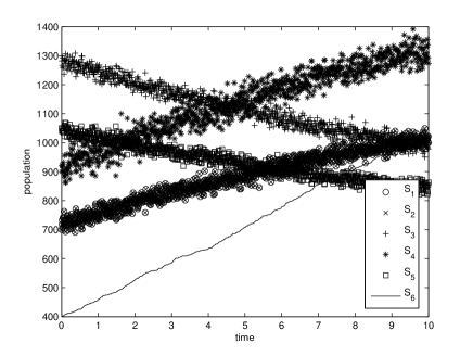
Figure 5: A trajectory of the jump process with initial condition (700,700,1300,900,1050,400).

The initial populations, $S_{1}(0),\dots,S_{6}(0)$ are drawn according to

$$\left(S_{1}(0),\dots,S_{6}(0)\right)=(700,700,1300,900,1050,400)+\eta$$

where $\eta$ is a vector of independent uniformly distributed random variables in the interval $[-10,10].$ The observations are taken every 1 unit of time from time 0 to time 10 and are modeled by

$$Z(l)=S(l)+\chi(l)$$

where the $\chi(l)$ are independent vectors of independent, mean 0, standard deviation 5, Gaussian random variables. While this noise model is somewhat arbitrary, it can be considered to model measurement error. In our experiments we take $z(l)$ to be equal to the particular trajectory shown in Figure 5 at time $l$ for $l=0,\dots,10.$

Because the standard particle filter is too expensive to run (almost 1000 times the cost of the multiscale particle filter) it is not available for comparison. However, we can still investigate the variance reduction aspect of the method by comparing two filters that both use the multiscale integration scheme during the prediction step, but that handle the update step in different ways. These two procedures are described in the next paragraph. For the details of the implementation of the multiscale integration scheme applied here please see [12, 13].

The two particle filters applied here correspond roughly to algorithms III.1 and III.2. In the first, at iteration $l$, we apply the multiscale integration scheme during the prediction step (thereby generating an approximate sample, ${S^{\prime}}^{j}_{6}(l)$ from $\bar{Q}_{\Delta s}$) then we choose one sample ${S^{\prime}}^{j}_{f}$ approximately from the measure $\mu_{{S^{\prime}}^{j}_{6}(l)}$ and proceed as in the rest of algorithm III.1. The latter sampling step is accomplished by sampling the end point from a long ($10^{-4}$ time units) equilibrated trajectory of the fast dynamics with the value ${S^{\prime}}^{j}_{6}(l)$ set as a parameter. The second method (corresponding to III.2) proceeds in exactly the same way except that in the second step we sample $10^{4}$ points ${S^{\prime}}^{j}_{f,m},$ at equal time intervals, from a long (again $10^{-4}$ time units) equilibrated trajectory of the fast dynamics with the value ${S^{\prime}}^{j}_{6}(l)$ set as a parameter. The points ${S^{\prime}}^{j}_{f,m}$ are then used to approximate the two averages appearing in Step 3 of algorithm III.2. With the severe scale separation present in this problem, the variance of the first method just described (no likelihood weight averaging) is an accurate representation of the variance of the standard particle filter. The increased cost of the averaging in the second method is negligible.

Both particle filters are tested with 1000 particles. The resulting estimators,

$$e^{1}_{i}(l)=\frac{W_{1}s_{i}\,(l)}{W_{1}1\,(l)}\qquad\text{and}\qquad e^{2}_{i}(l)=\frac{W_{2}s_{i}\,(l)}{W_{2}1\,(l)}$$

where, for any function $f,$

$$W_{1}f\,(l)=\frac{1}{n}\sum_{j=1}^{n}f({S^{\prime}}^{j}_{6}(l),{S^{\prime}}^{j}_{f})\,g({S^{\prime}}^{j}_{6}(l),{S^{\prime}}^{j}_{f},z_{l}),$$

and

$$W_{2}f\,(l)=\\ \frac{1}{n10^{4}}\sum_{j=1}^{n}\sum_{m=1}^{10^{4}}f({S^{\prime}}^{j}_{6}(l),{S^{\prime}}^{j}_{f,m})\,g({S^{\prime}}^{j}_{6}(l),{S^{\prime}}^{j}_{f,m},z_{l}).$$

a.

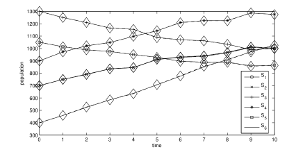
b.

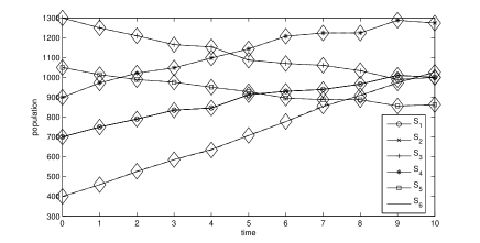
Figure 6: a. Trajectory of estimate $e^{1}$. b. Trajectory of estimate $e^{2}$. In both figures the observations are overlaid with diamonds connected by dashed lines.

of $S_{i}$ are plotted in Figure 6 along with the hidden trajectory of $S_{6}$. Clearly both methods accurately reconstruct the path of $S.$ Upon close inspection one can see that the estimate $e^{2}$ is slightly closer to the actual trajectory (which is the same as the observations in this example). However Figure 6 is by no means conclusive evidence that that $e^{2}$ provides a better estimate.

The gain in efficiency of the empirical measure generated using the averaged weights does become clear when we compare the effective sample sizes of the empirical measures produced by both methods,

$$ess_{1}=\frac{1000}{1+C^{2}_{1}}\quad\text{and}\quad ess_{2}=\frac{1000}{1+C^{2}_{2}}$$

where

$$C_{1}(l)=\frac{1}{W_{1}1\,(l)}\sqrt{\frac{1}{n}\sum_{j=1}^{n}\left(g({S^{\prime}}^{j}(l),{S^{\prime}}_{f}^{j},z_{l})-W_{1}1\,(l)\right)^{2}}$$

and

$$C_{2}(l)=\frac{1}{W_{2}1\,(l)}\sqrt{\frac{1}{n10^{4}}}\\ \times\sqrt{\sum_{j=1}^{n}\sum_{m=0}^{10^{4}}\left(g({S^{\prime}}^{j}_{6}(l),{S^{\prime}}^{j}_{f,m},z_{l})-W_{2}1\,(l)\right)^{2}}.$$

The trajectories of $ess_{1}$ and $ess_{2}$ are plotted in Figure 7.

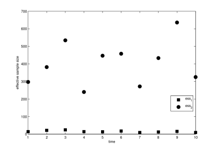
Figure 7: Trajectories of $ess_{1}$ and $ess_{2}.$

As can be seen in the plot, the effective sample sizes generated by the particle filter with averaging are as much as 100 times greater than those generated by the particle filter without the averaging step. This indicates that the improvement in the quality of the empirical measure generated by the particle filter with likelihood weight averaging is significant. It is also clear that, due to the large time scale separation in this system, any filtering method that does not explicitly address this in the prediction stage of the filter (by, for example, multiscale integration) will be extremely slow.

V Conclusions

We have presented an algorithm that combines dimensional reduction and approximate Rao-Blackwellization to create an efficient reduced variance particle filter for systems that exhibit time scale separation. We tested the algorithm on two systems with large time scale separations and the results are encouraging.

Our method does not require that any of the distributions involved are nearly Gaussian or degenerate. Furthermore, the cost of our method does not increase as the time scale separation is increased. We are not aware of any competitive alternative with these features.

With minor modifications our particle filter can be applied in a slightly more general setting. Occasionally one is interested in multiscale systems for which it is impossible to explicitly fix the slow variable during evolution. For example, one may not know the laws governing the evolution of the system but can generate sample trajectories (by laboratory experiment). In these cases our particle filter remains valid. Roughly, the fact that the slow variable does not deviate much on the time scale of the fast variables allows one to replace evolution of the fast dynamics by evolution of the full system (see [41]). Note also, that the variance reduction technique discussed here applies to any importance sampling problem for a multiscale Markov process.

VI Acknowledgments

We are grateful to Professor A.J. Chorin for suggesting the use of dimensional reduction in the context of filtering. We would like to thank Dr. Y. Shvets and the anonymous referees for helpful suggestions regarding this manuscript. This work was supported in part by the National Science Foundation under Grant DMS 04-32710, and by the Director, Office of Science, Computational and Technology Research, U.S. Department of Energy under Contract No. DE-AC03-76SF000098.

References

- [1] A.J. Chorin and P. Stinis. Problem reduction, renormalization, and memory. Comm. Appl. Math. Comp. Sc., 1:1–27, 2005.
- [2] D. Givon, R. Kupferman, and A. Stuart. Extracting macroscopic dynamics: model problems and algorithms. Nonlinearity, 17(6):R55–R127, 2004.
- [3] A. Doucet, N. de Freitas, and N. Gordon, editors. Sequential Monte Carlo methods in practice. Statistics for Engineering and Information Science. Springer-Verlag, New York, 2001.
- [4] A. J. Chorin and P. Krause. Dimensional reduction for a Bayesian filter. Proc. Natl. Acad. Sci. USA, 101(42):15013–15017 (electronic), 2004.
- [5] T. Kurtz. A limit theorem for perturbed operator semigroups with applications to random evolutions. J. Functional Analysis, 12:55–67, 1973.
- [6] G.C. Papanicolaou. Introduction to the Asymptotic Analysis of Stochastic Equations. In R.C. DiPrima, editor, Modern modeling of continuum phenomena, volume 16 of Lectures in Applied Mathematics, pages 109–148. AMS, 1977.
- [7] G. Pavliotis and A. Stuart. Multiscale Methods: Averaging and homoginization, volume 53 of Texts in Applied Mathematics. Springer, New York, 2008.
- [8] C. W. Gear and I. G. Kevrekidis. Projective methods for stiff differential equations: problems with gaps in their eigenvalue spectrum. SIAM J. Sci. Comput., 24(4):1091–1106 (electronic), 2003.
- [9] E. Vanden-Eijnden. Numerical techniques for multi-scale dynamical systems with stochastic effects. Commun. Math. Sci., 1(2):385–391, 2003.
- [10] Weinan E, Di Liu, and Eric Vanden-Eijnden. Analysis of multiscale methods for stochastic differential equations. Comm. Pure Appl. Math., 58(11):1544–1585, 2005.
- [11] D. Givon, I. G. Kevrekidis, and R. Kupferman. Strong convergence of projective integration schemes for singularly perturbed stochastic differential systems. Commun. Math. Sci., 4(4):707–729, 2006.
- [12] Y. Cao, D. Gillespie, and L. Petzold. The slow-scale stochastic simulation algorithm. J. Chem. Phys., 122(1):014116–18, 2005.
- [13] Weinan E, Di Liu, and Eric Vanden-Eijnden. Nested stochastic simulation algorithms for chemical kinetic systems with multiple time scales. J. Comput. Phys., 221(1):158–180, 2007.
- [14] Dror Givon and Ioannis G. Kevrekidis. Multiscale integration schemes for jump-diffusion systems. Multiscale Modeling and Simulation, 7(2):495–516, 2008.
- [15] S. Alizadeh, M. Brandt, and F. Diebold. Range-based estimation of stochastic volatility models. Journal of Finance, 57:1047–1091, 2002.
- [16] E. Haseltine and J. Rawlings. Approximate simulations of coupled fast and slow reactions for stochastic chemical kinetics. J. Chem. Phys., 117:6959–6969, 2002.
- [17] C. Rao and A. Arkin. Stochastic chemical kinetics and the quasisteady-state assumption: Application to the gillespie algorithm. J. Chem. Phys., 118:4999–5010, 2003.
- [18] R. Rico-Martinez, C. Gear, and I. Kevrekidis. Coarse projective kmc integration: forward/reverse initial and boundary value problems. J. Comput. Phys., 196:474–489, 2004.
- [19] Curtin W.A. and R.E. Miller. Atomistic/continuum coupling in computational materials science. Modelling and Simulation in Materials Science and Engineering, 11:R33–R68, 2003.
- [20] G. Martyna, M. Tuckerman, D. Tobias, and M. Klein. Explicit reversible integrators for extended systems dynamics. Mol. Phys., 87:1117–1157, 1996.
- [21] Carter E. Miller, R.N. and S. Blue. Data assimilation into nonlinear stochastic models. Tellus, 51A:167–194, 1999.
- [22] J. Weare. Particle filtering with path sampling and an application to a bimodal ocean current model. preprint.
- [23] A.J. Chorin, O.H. Hald, and R. Kupferman. Optimal prediction with memory. Physica D, 166:239–257, 2002.
- [24] H. Akashi and H. Kumamoto. Random sampling approach to state estimation in switching environments. Automatica, 13:429–434, 1977.
- [25] A. Doucet, S. Godsill, and C. Andrieu. On sequential monte carlo sampling methods for bayesian filtering. Statistics and Computing, 10:197–208, 2000.
- [26] A. Doucet, N. Gordon, and V. Krishnamurthy. Particle filters for state estimation of jump markov linear systems. IEEE Trans. Signal Processing, 49:613–624, 2001.
- [27] A. Kong, J. Liu, and W. Wong. Sequential imputations and bayesian missing data problems. J. Am. Stat. Assoc., 89:278–288, 1994.
- [28] J. Liu and R. Chen. Sequential monte carlo methods for dynamic systems. J. Am. Stat. Assoc., 93:1032–1044, 1998.
- [29] N. Vaswani. Pf-eis and pf-mt: New particle filtering algorithms for multimodal observation likelihoods and large dimensional state spaces. IEEE Intl. Conf. Acoustics, Speech, Sig. Proc., 2007.
- [30] A. Papavasiliou. Particle filters for multiscale diffusions. ESAIM Proceedings, 19:108–114, 2007.
- [31] H. J. Kushner. Weak convergence methods and singularly perturbed stochastic control and filtering problems, volume 3 of Systems & Control: Foundations & Applications. Birkhäuser Boston Inc., Boston, MA, 1990.
- [32] N. Gordon, D. Salmond, and C. Ewing. Novel approach to nonlinear/non-gaussian bayesian state estimation. IEEE Proceedings-F, 140:107–113, 1993.
- [33] M. I. Freidlin and A. D. Wentzell. Random perturbations of dynamical systems, volume 260 of Grundlehren der Mathematischen Wissenschaften [Fundamental Principles of Mathematical Sciences]. Springer-Verlag, New York, 1984. Translated from the Russian by Joseph Szücs.
- [34] P. Del Moral, J. Jacod, and P. Protter. The Monte-Carlo method for filtering with discrete- time observations. Probab. Theory Related Fields, 120(3):346–368, 2001.
- [35] R. Z. Khasminskiĭ. On the principle of averaging the Itô’s stochastic differential equations. Kybernetika (Prague), 4:260–279, 1968.
- [36] Christian P. Robert and George Casella. Monte Carlo statistical methods. Springer Texts in Statistics. Springer-Verlag, New York, second edition, 2004.
- [37] Stuart A.M. Mattingly, J.C. and D.J. Higham. Ergodicity for sdes and approximations: locally lipschitz vector fields and degenerate noise. Stochastic Processes and their Applications, 101:285–232, 1999.
- [38] G.O. Roberts and R.L. Tweedie. Exponential convergence of langevin diffusions and their discrete approximations. Bernoulli, 2:341–363, 1996.
- [39] J. Liu and R. Chen. Blind deconvolution via sequential imputations. J. Am. Stat. Assoc., 90(430):567–576, 1995.
- [40] D. T. Gillespie. A general method for numerically simulating the stochastic time evolution of coupled chemical reactions. Journal of Computational Physics, 22:403–434, 1976.
- [41] Ioannis G. Kevrekidis, C. William Gear, James M. Hyman, Panagiotis G. Kevrekidis, Olof Runborg, and Constantinos Theodoropoulos. Equation-free, coarse-grained multiscale computation: enabling microscopic simulators to perform system-level analysis. Commun. Math. Sci., 1(4):715–762, 2003.