Electromagnetic response of high-T_c superconductors –
the slave-boson and doped-carrier theories

Abstract

We evaluate the doping dependence of the quasiparticle current and low temperature superfluid density in two slave-particle theories of the $tt^{\prime}t^{\prime\prime}J$ model – the slave-boson theory and doped-carrier theory. In the slave-boson theory, the nodal quasiparticle current renormalization factor $\alpha$ vanishes proportionally to the zero temperature superfluid density $\rho_{S}(0)$; however, we find that away from the $\rho_{S}(0)\rightarrow 0$ limit $\alpha$ displays a much weaker doping dependence than $\rho_{S}(0)$. A similar conclusion applies to the doped-carrier theory, which differentiates the nodal and antinodal regions of momentum space. Due to its momentum space anisotropy, the doped-carrier theory enhances the value of $\alpha$ in the hole doped regime, bringing it to quantitative agreement with experiments, and reproduces the asymmetry between hole and electron doped cuprate superconductors. Finally, we use the doped-carrier theory to predict a specific experimental signature of local staggered spin correlations in doped Mott insulator superconductors which, we propose, should be observed in STM measurements of underdoped high-T_c compounds. This experimental signature distinguishes the doped-carrier theory from other candidate mean-field theories of high-T_c superconductors, like the slave-boson theory and the conventional BCS theory.

I Introduction

I.1 Motivation

The phenomenology of high-temperature superconducting (SC) cuprates is most striking when electron occupancy per unit cell is close to unity Timusk and Statt (1999). In this underdoped regime, the SC critical temperature (T_c) vanishes as the interaction-driven Mott insulator is approached despite the strong binding of electrons into Cooper pairs Wang et al. (2003); Krusin-Elbaum et al. (2004). This deviation from BCS theory is reflected in the anomalous metallic pseudogap state, whose Fermi surface appears to be partially gapped Norman et al. (1998); Kanigel et al. (2006). The physics that determines the value of T_c in underdoped cuprates is a highly debated Emery and Kivelson (1995); Lee and Wen (1997); Wen and Lee (1998); Wu et al. (1998); Balents et al. (1999); Lee (2000); Ioffe and Millis (2002); Herbut (2005); Lee et al. (2006); Franz and Iyengar (2006); CPO1 ; CPO2 ; Yeh fundamental question which lacks a fully satisfactory answer.

In this context, it is important to sort the specific roles played by phase fluctuations of the order parameter and by fermionic quasiparticle excitations in destroying superconductivity at finite temperatures. Since the zero temperature superfluid phase stiffness $\rho_{S}(0)$ decreases together with T_c Uemura et al. (1989); Boyce et al. (2000); Pereg-Barnea et al. (2004); Liang et al. (2005); Zuev et al. (2005); Broun et al. (2005), phase fluctuations are certainly detrimental to long-range phase coherence Emery and Kivelson (1995), as evidenced by the magnetic vortices observed in the normal state Xu et al. (2000). Yet, to reconcile T_c with the measured bare phase stiffness Corson et al. (1999) requires that thermally excited nodal quasiparticles reduce $\rho_{S}$, thus promoting vortex proliferation at a temperature lower than expected from phase-only arguments Lee and Wen (1997); Ioffe and Millis (2002); Lee et al. (2006). The important role played by the $d_{x^{2}-y^{2}}$-wave quasiparticles receives further experimental support from penetration depth measurements in underdoped YBCO films which display characteristic quasiparticle behavior, namely the linear in $T$ suppression of $\rho_{S}$, up to $T\gtrsim\text{T}_{c}/2$ (see, for instance, Fig. 1 of Ref. Boyce et al., 2000). Remarkably, this $T$-linear regime extends all the way to T_c in severely underdoped samples which, in addition, violate the $\text{T}_{c}\propto\rho_{S}(0)$ relation applicable in pure phase-fluctuation models Pereg-Barnea et al. (2004); Liang et al. (2005); Zuev et al. (2005); Broun et al. (2005). The above strongly supports that the T_c scale in underdoped cuprates is set by the effective parameters $\rho_{S}(0)$ and $d\rho_{S}/dT$. Simultaneously describing the above two parameters in consistency with experiments is the main problem we address in this paper.

In the remaining of this introductory section, we illustrate that present theoretical understanding cannot easily reconcile the experimentally observed behavior of $\rho_{S}(0)$ with that of $d\rho_{S}/dT$ (Sec. I.2). The latter parameter reflects the interaction induced renormalization of the quasiparticle current and, as such, in Sec. I.3 we discuss how interactions are expected to renormalize the quasiparticle current throughout the entire Brillouin zone. We also note that these renormalization effects can be probed by scanning tunneling microscopy (STM) experiments, which can provide valuable information to distinguish between different quasiparticle descriptions of underdoped curpates. Finally, in Sec. I.4 we present the layout of the full paper.

I.2 The effective parameters $\rho_{S}(0)$ and $d\rho_{S}/dT$

The effective parameter $\rho_{S}(0)$ quantifies the coupling between an applied gauge field and the superconducting condensate, as evidenced in the Meissner effect. The depletion of $\rho_{S}(0)$ as the Mott insulator is approached Uemura et al. (1989); Boyce et al. (2000); Pereg-Barnea et al. (2004); Liang et al. (2005); Zuev et al. (2005); Broun et al. (2005) is in stark contrast with the prediction from BCS theory, namely $\rho_{S}(0)\propto 1-x$, where $x$ is the density of carriers doped away from half-filling. This sharp deviation follows from the large Coulomb repulsion that suppresses (enhances) charge (phase) fluctuations and, indeed, the observed $\rho_{S}(0)\sim x$ behavior is captured by the slave-boson (SB) theory of the $tJ$ model Wen and Lee (1996); Lee et al. (1998, 2006), which is a microscopic approach that explicitly implements the suppression of charge fluctuations. The same behavior is encountered in theories of phase fluctuating $d$-wave superconductors Wu et al. (1998); Balents et al. (1999); Herbut (2005); Franz et al. (2002); Herbut (2002), whose effective theory is similar to that of the SB approach Wu et al. (1998); Herbut (2005). However, the above success in reproducing $\rho_{S}(0)\sim x$ is not accompanied by a similar fate when it comes to addressing $d\rho_{S}/dT$’s experimental results. In fact, the microscopic SB approach predicts too small values of $d\rho_{S}/dT$ in the limit $x\rightarrow 0$.

The parameter $d\rho_{S}/dT$ is often characterized in terms of the nodal current renormalization factor $\alpha\equiv[(2\pi v_{\Delta}/v_{F}\ln 2)\,d\rho_{S}/dT]^{1/2}$, where $v_{F}$ and $v_{\Delta}$ are the Fermi and gap velocities respectively. In the BCS theory, $\alpha=1$. In the SB theory, however, the effect of Coulomb repulsion leads to $\alpha\sim\rho_{S}(0)$ in the limit $x\rightarrow 0$ Lee and Wen (1997); Lee et al. (2006); Lee (2000); Herbut (2005). This is commonly regarded as a major setback since experiments show that $\alpha$ vanishes sublinearly in $\rho_{S}(0)$ Liang et al. (2005); Zuev et al. (2005); Broun et al. (2005). In addition, it casts doubt on the applicability of the SB formalism to simultaneously describe how SC quasiparticles and the SC condensate couple to an applied electromagnetic field.

We remark that the above mismatch between the SB theory and experiments occurs in the limit $x\rightarrow 0$, in which case the SB theory ignores the emergence of the antiferromagnetic (AF) phase. Therefore, in this paper we extend previous work in the literature that uses the slave-particle framework to address the superfluid density $\rho_{S}$ in the limit $x\rightarrow 0$ Lee and Wen (1997); Wen and Lee (1998); Lee (2000), and calculate the low energy and long wavelength electromagnetic response function of a doped Mott insulator superconductor away from the above limit. We specifically consider two slave-particle theories of the $tt^{\prime}t^{\prime\prime}J$ model, namely the SB and the doped-carrier (DC) theories Wen and Lee (1996); Lee et al. (1998); Ribeiro and Wen (2005, 2006a), for which we calculate the nodal current renormalization factor $\alpha$ as a function of $x$. We argue that, in this respect, slave-particle theories may compare to experiments better than often thought. In fact, we find that both the SB and the DC slave-particle approaches predict that, for $x\gtrsim 0.05$ and in the considered parameter range $2J\leq t\leq 5J$, the doping dependence of $\alpha$ is much weaker than that of $\rho_{S}(0)$, in agreement with underdoped cuprates’ data Boyce et al. (2000).

I.3 Renormalized quasiparticle current distribution

As we state above, superfluid density measurements probe the quasiparticle current renormalization at the nodal points of $d_{x^{2}-y^{2}}$-wave superconductors. Interactions, however, also renormalize the current of quasiparticles away from the nodes, an effect which should manifest itself in experiments, as we overview in what follows.

We know that a finite supercurrent $\bm{J}_{s}$ shifts the superconducting quasiparticle dispersion $E_{\bm{k}}$ and, to linear order in $\bm{J}_{s}$, we have

$$E_{\bm{k}}(\bm{A})=E_{\bm{k}}(0)-\bm{j}_{\bm{k}}\cdot\bm{A}$$ (1)

where we introduce the vector potential $\bm{A}$ to represent the supercurrent $\bm{J}_{s}=\rho_{S}\bm{A}$. [Note that in Eq. (1) we set the speed of light to $c=1$; in what follows, we also take the electric charge to be $e=1$, as well as $\hbar=1$.] The (hole) quasiparticle current $\bm{j}_{\bm{k}}$ characterizes how excited quasiparticles affect the superfluid density $\rho_{S}$ and, in the BCS theory, it is given by the expression

$$\bm{j}_{\bm{k}}=-\frac{\partial\epsilon_{\bm{k}}^{N}}{\partial\bm{k}}$$ (2)

where $\epsilon_{\bm{k}}^{N}$ is the normal state (hole) energy dispersion which, in the present discussion, we approximate by $\epsilon_{\bm{k}}^{N}=2t[\cos(k_{x})+\cos(k_{y})]$. [Up to a constant scale factor, Fig. 1(a) resembles this quasiparticle current distribution.]

We note that, according to the BCS theory, the quasiparticle current $\bm{j}_{\bm{k}}$ is completely determined by the normal state dispersion (this applies all the way deep into the superconducting state). Since, at many levels, the phenomenology of overdoped cuprates is compatible with the BCS theory, we still expect Eq. (2) to hold in these samples, with $\epsilon_{\bm{k}}^{N}$ given by the appropriate free electron dispersion. However, the free electron dispersion should not be used to calculate the quasiparticle current of superconducting underdoped cuprates. This then raises the question of what normal state dispersion we should use to calculate the quasiparticle current distribution $\bm{j}_{\bm{k}}$ in underdoped cuprates. The answer to this question may come from angle-resolved photoemission spectroscopy (ARPES) experiments in half-filled cuprate compounds showing that the single hole dispersion is roughly given by $\epsilon^{AF}_{\bm{k}}\propto[\cos(2k_{x})+\cos(2k_{y})]$ Wells et al. (1995), in which case the quasiparticle current $\bm{j}_{\bm{k}}=-\tfrac{\partial\epsilon^{AF}_{\bm{k}}}{\partial\bm{k}}$ [see Fig. 1(f)] considerably differs from the BCS-like result in Fig. 1(a). This suggests that, perhaps, in the cuprates’ underdoped regime we should use a quasiparticle current derived from a dispersion that interpolates between $\epsilon_{\bm{k}}^{N}$ and $\epsilon^{AF}_{\bm{k}}$.

From the above discussion, we see that the quasiparticle current distribution $\bm{j}_{\bm{k}}$ is an important quantity that can reveal new characteristics of underdoped high-T_c superconductors which lie beyond the BCS paradigm. Hence, it is relevant to calculate and predict $\bm{j}_{\bm{k}}$ using different approaches to the high-T_c problem. It is also significant to experimentally measure $\bm{j}_{\bm{k}}$, as such a measurement could prove to be instrumental in either ruling out or validating candidate theories to the high-T_c problem.

As a step in this direction, below we calculate the quasiparticle current distribution using two different approaches, namely the aforementioned SB and DC approaches. We find that these yield quite distinct distributions of the quasiparticle current throughout the Brillouin zone [see Figs. 1(a) and 1(c)]. The mean-field SB approach gives rise to a quasiparticle current distribution which, in the absence of intra-sublattice hopping processes, is essentially the BCS result multiplied by the current renormalization factor $\alpha$. The DC approach results in a quasiparticle current distribution which, instead, interpolates between the BCS and AF current distributions $\bm{j}_{\bm{k}}=-\tfrac{\partial\epsilon_{\bm{k}}^{N}}{\partial\bm{k}}$ and $\bm{j}_{\bm{k}}=-\tfrac{\partial\epsilon^{AF}_{\bm{k}}}{\partial\bm{k}}$, respectively.

In this paper, we propose that measuring the tunneling differential conductance from a metal tip into the superconducting $C_{u}O$ plane in the presence of a supercurrent provides a way to distinguish the above quasiparticle current distributions. Specifically, we calculate how the tunneling differential conductance is affected by an applied supercurrent in the $C_{u}O$ plane, and find that the different quasiparticle current distributions lead to different supercurrent dependences of the tunneling differential conductance (see Fig. 4). We further argue that this effect may be probed by STM experiments, which thus could distinguish the DC theory description of high-T_c superconducors from alternative theories (particularly those that ignore the momentum space differentiation of the nodal and antinodal regions, such as the SB theory and the conventional BCS theory).

I.4 Paper layout

The paper is organized as follows. In Sec. II we introduce the formalism used to calculate the low energy and long wavelength electromagnetic response function within the SB and DC frameworks. In order to obtain the non-zero temperature electromagnetic response function in the static and uniform limit we follow Ioffe and Larkin Ioffe and Larkin (1989) and resort to the random-phase approximation (RPA), which accounts for the effect of fluctuations around the mean-field saddle point up to Gaussian level. This calculation yields the doping dependent quasiparticle current and $\rho_{S}(T)$ low temperature behavior in the SB and DC theories, whose results we discuss and compare in Sec. III. In this section, we also study the parametric dependence of $\rho_{S}(T)$ on $t/J$ values. In the DC framework we use in this paper, the momentum space anisotropy follows from the role of high-energy AF correlations between local moments in superconducting doped Mott insulators. Hence, the aforementioned comparison between the SB and the DC theory results identifies the effect of short-range AF correlations in the electromagnetic response of a $d$-wave superconductor close to a Mott insulator transition. We conclude that AF correlations enhance (suppress) the nodal quasiparticle current in the hole (electron) doped regime of cuprate superconductors. In the hole doped case, and for $t/J=3$, that enhancement leads to $0.5\lesssim\alpha\lesssim 0.6$ when $0.1\lesssim x\lesssim 0.2$, in quantitative agreement with experiments Mesot et al. (1999); Chiao et al. (2000); Hawthorn et al. (2003). In this doping range, the DC theory quasiparticle-driven T_c scale T${}_{c}^{QP}\equiv\rho_{S}(0)/(d\rho_{S}/dT)\sim J/10$ is an order of magnitude lower than in the SB theory and, in addition, it agrees with the cuprates’ T_c scale. Our results also show that the intriguing weak temperature dependence of $\rho_{S}(T)$ in electron doped compounds Alff et al. (1999); Kim et al. (2003) is consistent with the observed momentum space anisotropy Armitage et al. (2002), which we consider to follow from the strong local AF correlations. Since the formalism introduced in Sec. II also allows one to study the coupling between the SC quasiparticles and an applied supercurrent, in Sec. IV we use this fact to predict a specific experimental signature of a traversing supercurrent in the tunneling differential conductance that, we propose, should be detected in STM measurements.

II Formalism

We set to calculate the low energy and long wavelength electromagnetic response function of a doped Mott insulator superconductor. In particular, we consider two different families of slave-particle wave functions, one described by the SB $d$-wave SC ansatz Wen and Lee (1996); Lee et al. (1998) and the other by the DC $d$-wave SC ansatz Ribeiro and Wen (2005, 2006a). In addition, we choose the energetics to be given by the $tt^{\prime}t^{\prime\prime}J$ model Hamiltonian

$$H_{tJ}=\sum_{\langle ij}J_{ij}\bm{S}_{i}.\bm{S}_{j}-\sum_{\langle ij\rangle,\sigma}t_{ij}(\tilde{c}_{i,\sigma}^{\dagger}\tilde{c}_{j,\sigma}+h.c.)$$ (3)

where $\tilde{c}_{i,\sigma}^{\dagger}=c_{i,\sigma}^{\dagger}(1-c_{i,-\sigma}^{\dagger}c_{i,-\sigma})$ are the Gutzwiller projected electron operators, $\bm{S}_{i}=\tilde{c}_{i}^{\dagger}\bm{\sigma}\tilde{c}_{i}$ are the electron spin operators and $\bm{\sigma}$ are the Pauli matrices. Also, $J_{ij}=J$ for NN sites, and $t_{ij}=t,t^{\prime},t^{\prime\prime}$ for first, second and third NN sites, respectively. Since the SC nodal quasiparticles are the sole gapless excitations, below we resort to the SB (Sec. II.1) and DC (Sec. II.2) mean-field theories. In both cases, we include the effect of gapped collective modes at the RPA level.

II.1 Slave-boson framework

We first determine how the well studied Wen and Lee (1996); Lee and Wen (1997); Lee et al. (1998); Wen and Lee (1998); Lee and Nagaosa (2003); Lee et al. (2006) SB $d$-wave superconductor couples to an applied electromagnetic field. In the $SU(2)$ SB framework the projected electron operators are decoupled as $\tilde{c}_{i,\uparrow}^{\dagger}=\tfrac{1}{\sqrt{2}}\psi_{i}^{\dagger}h_{i}$ and $\tilde{c}_{i,\downarrow}^{\dagger}=\tfrac{1}{\sqrt{2}}\psi_{i}^{T}(-i\sigma_{2})h_{i}$, where $\psi_{i}$ are the chargeless and spin-1/2 spinon fermionic operators in the Nambu representation, and $h_{i}$ are the spinless and charge-$e$ holon bosonic operators Wen and Lee (1996). If one rewrites Eq. (3) in terms of $\psi_{i}$ and $h_{i}$, and further applies the Hartree-Fock-Bogoliubov decoupling scheme, one obtains the quadratic SB mean-field Hamiltonian $H_{MF}^{SB}=H_{\psi}^{SB}+H_{h}^{SB}$, where Ribeiro and Wen (2003):

$$\begin{split}H_{\psi}^{SB}&=\sum_{\langle ij\rangle}\frac{3J_{ij}}{16}Tr\left[U_{ij}U_{ji}\right]+\bm{a}_{0}.\Bigl{(}\sum_{i}\psi_{i}^{\dagger}\bm{\sigma}\psi_{i}\Bigr{)}-\\ &\quad-\sum_{\langle ij\rangle}\Bigl{[}\psi_{i}^{\dagger}\Bigl{(}\frac{3J_{ij}}{8}U_{ij}+\frac{t_{ij}}{2}V_{ij}\Bigr{)}\psi_{j}+h.c.\Bigr{]}\end{split}$$ (4)

$$\begin{split}H_{h}^{SB}&=\sum_{\langle ij\rangle}\frac{t_{ij}}{2}Tr\left[U_{ij}V_{ji}\right]+\bm{a}_{0}.\Bigl{(}\sum_{i}h_{i}^{\dagger}\bm{\sigma}h_{i}\Bigr{)}-\\ &\quad-\mu_{h}\sum_{i}h_{i}^{\dagger}h_{i}-\sum_{\langle ij\rangle}\frac{t_{ij}}{2}\Bigl{(}h_{i}^{\dagger}U_{ij}h_{j}+h.c.\Bigr{)}\end{split}$$ (5)

The holon chemical potential $\mu_{h}$ controls the density $\langle h_{i}^{\dagger}h_{i}\rangle=x$ and the Lagrange multiplier $\bm{a}_{0}=a_{0}\sigma_{3}$ implements the $SU(2)$ projection constraint at mean-field level $\langle\psi_{i}^{\dagger}\bm{\sigma}\psi_{i}+h_{i}^{\dagger}\bm{\sigma}h_{i}\rangle=0$. In the $d$-wave SC ansatz $h_{i}^{\dagger}=[h\ 0]$, where $h$ is the holon condensate magnitude, $V_{ij}=x\sigma_{3}$, $U_{i\,i+\hat{x}}=\chi\sigma_{3}+\Delta\sigma_{1}$, and $U_{i\,i+\hat{y}}=\chi\sigma_{3}-\Delta\sigma_{1}$.

Since only holons carry electric charge, minimally coupling an electromagnetic gauge field $A_{ij}$ to $H_{MF}^{SB}$ amounts to replacing $h_{i}^{\dagger}U_{ij}h_{j}$ in Eq. (5) by $h_{i}^{\dagger}U_{ij}\exp(iA_{ij})h_{j}$. In order to account for the effect of fluctuations around mean-field we also must replace $U_{ij}$ and $V_{ij}$ in Eqs. (4) and (5) by $[\tfrac{1}{2}U_{ij}\exp(i\bm{a}_{ij}.\bm{\sigma})+\tfrac{1}{2}\exp(i\bm{a}_{ij}.\bm{\sigma})U_{ij}]$ and $[\tfrac{1}{2}V_{ij}\exp(i\bm{a}_{ij}.\bm{\sigma})+\tfrac{1}{2}\exp(i\bm{a}_{ij}.\bm{\sigma})V_{ij}]$, respectively, where $\bm{a}_{ij}$ is the $SU(2)$ gauge field that describes collective modes in the SB framework Lee et al. (1998); Lee and Nagaosa (2003); Lee et al. (2006). In what follows, we consider the resulting minimally coupled Hamiltonian $H_{MF}^{SB}(A_{ij},\bm{a}_{ij})$ in the static and uniform limit, and thus recast $A_{i+\vec{u}\,i}\equiv A_{\hat{x}}\,\vec{u}.\hat{x}+A_{\hat{y}}\,\vec{u}.\hat{y}$ and $\bm{a}_{i+\vec{u}\,i}\equiv\bm{a}_{\hat{x}}\,\vec{u}.\hat{x}+\bm{a}_{\hat{y}}\,\vec{u}.\hat{y}$.

If we ignore the contribution from collective modes, the electromagnetic current and response function are $J_{A,\hat{u}}^{SB}=-\tfrac{1}{N}\left.\tfrac{\partial F^{SB}(A,\bm{a})}{\partial A_{\hat{u}}}\right|_{A,\bm{a}=0}$ and $\Pi_{AA,\hat{u}\hat{v}}^{SB}=\tfrac{1}{N}\left.\tfrac{\partial^{2}F^{SB}(A,\bm{a})}{\partial A_{\hat{u}}\,\partial A_{\hat{v}}}\right|_{A,\bm{a}=0}$, where $F^{SB}(A,\bm{a})$ is the free-energy obtained from $H_{MF}^{SB}(A_{ij},\bm{a}_{ij})$. However, as shown by Ioffe and Larkin Ioffe and Larkin (1989), the above modes are important to correctly determine how strongly correlated superconductors couple to the electromagnetic field. In the SC state these modes are gapped and we only keep free-energy terms up to quadratic order in $\bm{a}_{\hat{u}}$. Integrating out $\bm{a}_{\hat{u}}$, we obtain the electromagnetic current and response function within RPA, namely,

$$J^{SB}\,=\,J_{A}^{SB}-\,\,\bm{\Pi}_{Aa}^{SB}.\left(\bm{\Pi}_{aa}^{SB}\right)^{-1}\!\!.\,\,\bm{J}_{a}^{SB}$$ (6)

$$\Pi^{SB}\,=\,\Pi_{AA}^{SB}-\,\,\bm{\Pi}_{Aa}^{SB}.\left(\bm{\Pi}_{aa}^{SB}\right)^{-1}\!\!.\,\,\bm{\Pi}_{aA}^{SB}$$ (7)

where $\bm{J}_{a,\hat{u}}^{SB}=-\tfrac{1}{N}\left.\tfrac{\partial F^{SB}(A,\bm{a})}{\partial\bm{a}_{\hat{u}}}\right|_{A,\bm{a}=0}$, $\left(\bm{\Pi}_{aA,\hat{v}\hat{u}}^{SB}\right)^{\dagger}=\bm{\Pi}_{Aa,\hat{u}\hat{v}}^{SB}=\tfrac{1}{N}\left.\tfrac{\partial^{2}F^{SB}(A,\bm{a})}{\partial A_{\hat{u}}\,\partial\bm{a}_{\hat{v}}}\right|_{A,\bm{a}=0}$, and $\bm{\Pi}_{aa,\hat{u}\hat{v}}^{SB}=\tfrac{1}{N}\left.\tfrac{\partial^{2}F^{SB}(A,\bm{a})}{\partial\bm{a}_{\hat{u}}\,\partial\bm{a}_{\hat{v}}}\right|_{A,\bm{a}=0}$. We note that $J_{A,\hat{u}}^{SB}$ and $\bm{J}_{a,\hat{u}}^{SB}$ correspond to the sums over momentum space $J_{A,\hat{u}}^{SB}=\tfrac{1}{N}\sum_{b,\bm{k}}n_{b,\bm{k}}\,j_{b,\bm{k},\hat{u}}^{A,SB}$ and $\bm{J}_{a,\hat{u}}^{SB}=\tfrac{1}{N}\sum_{b,\bm{k}}n_{b,\bm{k}}\,\bm{j}_{b,\bm{k},\hat{u}}^{a,SB}$, where $n_{b,\bm{k}}$ is the occupation number of the mean-field single particle state in band $b$ and with momentum $\bm{k}$, whose energy dispersion $\epsilon_{b,\bm{k}}^{SB}(A,\bm{a})$ implies the quasiparticle current components $j_{b,\bm{k},\hat{u}}^{A,SB}=-\tfrac{\partial\epsilon_{b,\bm{k}}^{SB}(A,\bm{a})}{\partial A_{\hat{u}}}$ and $\bm{j}_{b,\bm{k},\hat{u}}^{a,SB}=-\tfrac{\partial\epsilon_{b,\bm{k}}^{SB}(A,\bm{a})}{\partial\bm{a}_{\hat{u}}}$. Following the above formula, we introduce the SB theory quasiparticle current (within RPA)

$$j_{b,\bm{k},\hat{u}}^{SB}\,\equiv\,\frac{\partial J_{\hat{u}}^{SB}}{\partial n_{b,\bm{k}}}\,=\,j_{b,\bm{k},\hat{u}}^{A,SB}-\,\,\bm{\Pi}_{Aa}^{SB}.\left(\bm{\Pi}_{aa}^{SB}\right)^{-1}\!\!.\,\,\bm{j}_{b,\bm{k},\hat{u}}^{a,SB}$$ (8)

where we use $\bm{J}_{a,\hat{u}}^{SB}=0$, which applies in thermal equilibrium and in the absence of external fields. Eq. (8) is equivalent to $j_{b,\bm{k},\hat{u}}^{SB}=-\tfrac{dE_{b,\bm{k}}^{SB}(A)}{dA_{\hat{u}}}$, where $E_{b,\bm{k}}^{SB}(A)=\epsilon_{b,\bm{k}}^{SB}(A,\bm{a})|_{\bm{a}=-\left(\bm{\Pi}_{aa}^{SB}\right)^{-1}\!\!.\,\,\bm{\Pi}_{aA}^{SB}\,A}$ is the single particle dispersion obtained in the presence of an applied gauge field $A_{\hat{u}}$ after integrating out $\bm{a}_{\hat{u}}$. We additionally obtain the SB theory superfluid density (within RPA) $\rho_{S}^{SB}$ from $\Pi_{\hat{u}\hat{v}}^{SB}=\rho_{S}^{SB}\delta_{\hat{u}\hat{v}}$ GAU .

II.2 Doped-carrier framework

We now determine how an applied electromagnetic field couples to the DC $d$-wave SC state in the static and uniform limit. The only difference when compared to the SB approach sketched in Sec. II.1 has to do with the specific decoupling of the Gutzwiller projected electron operators which, in the DC framework, read Ribeiro and Wen (2006a) $\tilde{c}_{i,\sigma}^{\dagger}=s_{\sigma}\tfrac{1}{\sqrt{2}}\left[\left(\tfrac{1}{2}+s_{\sigma}\widetilde{S}_{i}^{z}\right)\tilde{d}_{i,-\sigma}-\widetilde{S}_{i}^{s_{\sigma}}\tilde{d}_{i,\sigma}\right]$. Here, $s_{\sigma}=(+1),(-1)$ for $\sigma=\uparrow,\downarrow$. $\tilde{d}_{i,\sigma}=d_{i,\sigma}(1-d_{i,-\sigma}^{\dagger}d_{i,-\sigma})$ is the charge-$e$ and spin-1/2 projected doped carrier operator ($d_{i}$, which has the same quantum numbers as the holes doped into the Mott insulator, has been called the dopon operator in Ref. Ribeiro and Wen, 2005). Further writing the above spin operators in terms of chargeless spin-1/2 spinons as $\widetilde{\bm{S}}_{i}=\tfrac{1}{2}f_{i}^{\dagger}\bm{\sigma}f_{i}$ leads to the DC mean-field Hamiltonian $H_{MF}^{DC}=H_{\psi}^{DC}+H_{\eta}^{DC}+H_{mix}^{DC}$, where Ribeiro and Wen (2005, 2006a):

$$\begin{split}H_{\psi}^{DC}&=\frac{3\tilde{J}}{16}\!\!\sum_{\langle ij\rangle\in NN}\!\!Tr\left[U_{ij}U_{ji}\right]+\bm{a}_{0}.\Bigl{(}\sum_{i}\psi_{i}^{\dagger}\bm{\sigma}\psi_{i}\Bigr{)}-\\ &\quad-\!\!\!\!\!\sum_{\langle ij\rangle\in NN}\Bigl{[}\psi_{i}^{\dagger}\Bigl{(}\frac{3\tilde{J}}{8}U_{ij}-\frac{t_{1}x}{2}\sigma_{3}\Bigr{)}\psi_{j}+h.c.\Bigr{]}\end{split}$$ (9)

$$H_{\eta}^{DC}=\sum_{i}\sum_{\nu=2,3}\sum_{\vec{u}\in\nu\,NN}\frac{t_{\nu}}{4}\eta_{i+\vec{u}}^{\dagger}\sigma_{3}\eta_{i}-\mu_{d}\sum_{i}\eta_{i}^{\dagger}\sigma_{3}\eta_{i}$$ (10)

$$\begin{split}H_{mix}^{DC}&=-\sum_{i}Tr\left[B_{i1}^{\dagger}B_{i0}\right]-\sum_{i}\left(\eta_{i}^{\dagger}B_{i1}\psi_{i}+h.c.\right)\\ &\ \ \ -\frac{3}{16}\sum_{i,\nu}\sum_{\vec{u}\in\nu\,NN}t_{\nu}\left(\eta_{i+\vec{u}}^{\dagger}B_{i0}\psi_{i}+h.c.\right)\end{split}$$ (11)

Above, $\psi_{i}$ and $\eta_{i}$ are the spinon and dopon operators in the Nambu representation. $\vec{u}=\pm\hat{x},\pm\hat{y}$, $\vec{u}=\pm\hat{x}\pm\hat{y}$ and $\vec{u}=\pm 2\hat{x},\pm 2\hat{y}$ for $\nu=1,2,3$ respectively. $\mu_{d}$ is the chemical potential that sets the doped carrier density $x$. $\tilde{J}=(1-x)^{2}J$, $t_{1}=t$, $t_{2}=J+(1-x/0.3)t^{\prime}$ and $t_{3}=J/2+(1-x/0.3)t^{\prime\prime}$, where $J$, $t$, $t^{\prime}$ and $t^{\prime\prime}$ parameterize the $tt^{\prime}t^{\prime\prime}J$ model Hamiltonian. In the $d$-wave SC ansatz, $U_{i\,i+\hat{x}}=\chi\sigma_{3}+\Delta\sigma_{1}$, $U_{i\,i+\hat{y}}=\chi\sigma_{3}-\Delta\sigma_{1}$, $B_{i0}=-b_{0}\sigma_{3}$ and $B_{i1}=-b_{1}\sigma_{3}$. Furthermore, the Lagrange multiplier $\bm{a}_{0}=a_{0}\sigma_{3}$ sets $\langle\psi_{i}^{\dagger}\bm{\sigma}\psi_{i}\rangle=0$. As shown in Ref. Ribeiro and Wen, 2006a, the SB and the DC formulations are related to each other since the local singlet state of a dopon $d_{i}$ and a spinon $f_{i}$ in the DC approach corresponds to the holon in the SB approach. Consequently, the DC theory mean-field $b_{0}=\langle f_{i}^{\dagger}d_{i}\rangle$ is equivalent to the SB holon condensate magnitude $h$.

In this paper, we extend previous work on the DC framework and introduce the electromagnetic gauge field $A_{ij}$, as well as the fluctuations around the $U_{ij}$ mean-field described by the $SU(2)$ gauge modes $\bm{a}_{ij}$ (analogous to those in the SB formulation). Before constructing the minimally coupled Hamiltonian $H_{MF}^{DC}(A_{ij},\bm{a}_{ij})$, we summarize how the fields in Eqs. (9), (10) and (11) transform under $U(1)$ electromagnetic gauge transformations and under $SU(2)$ gauge transformations associated with the $\bm{a}_{ij}$ modes: (i) $\psi_{i}$ is an on-site field which carries no electric charge and which is in the $SU(2)$ fundamental representation; (ii) $\eta_{i}$ is an on-site field which carries electric charge and is invariant to $SU(2)$ gauge transformations; (iii) $B_{i0}$ is an on-site field which carries electric charge and which is in the $SU(2)$ fundamental representation; (iv) $U_{ij}$ is defined on the lattice bonds, carries no electric charge and is in the $SU(2)$ adjoint representation. As a result, $H_{MF}^{DC}(A_{ij},\bm{a}_{ij})$ is obtained from $H_{MF}^{DC}$ by replacing: (i) $\ (\tfrac{3\tilde{J}}{8}U_{ij}-\tfrac{t_{1}x}{2}\sigma_{3})$ in Eq. (9) by $\tfrac{1}{2}(\tfrac{3\tilde{J}}{8}U_{ij}-\tfrac{t_{1}x}{2}\sigma_{3})\exp{(i\bm{a}_{ij}.\bm{\sigma})}+\tfrac{1}{2}\exp{(i\bm{a}_{ij}.\bm{\sigma})}(\tfrac{3\tilde{J}}{8}U_{ij}-\tfrac{t_{1}x}{2}\sigma_{3})$; (ii) $\ \eta_{i+\vec{u}}^{\dagger}\sigma_{3}\eta_{i}$ in Eq. (10) by $\eta_{i+\vec{u}}^{\dagger}\exp{(iA_{i+\vec{u}\,i}\sigma_{3})}\sigma_{3}\eta_{i}$; (iii) $\ \eta_{i+\vec{u}}^{\dagger}B_{i0}\psi_{i}$ in Eq. (11) by $\eta_{i+\vec{u}}^{\dagger}\exp{(iA_{i+\vec{u}\,i}\sigma_{3})}B_{i0}\psi_{i}$. Similarly to Sec. II.1, we further recast $A_{i+\vec{u}\,i}\equiv A_{\hat{x}}\,\vec{u}.\hat{x}+A_{\hat{y}}\,\vec{u}.\hat{y}$ and $\bm{a}_{i+\vec{u}\,i}\equiv\bm{a}_{\hat{x}}\,\vec{u}.\hat{x}+\bm{a}_{\hat{y}}\,\vec{u}.\hat{y}$.

Given $H_{MF}^{DC}(A_{ij},\bm{a}_{ij})$, we can determine the DC mean-field free-energy $F^{DC}(A,\bm{a})$, from which the DC electromagnetic current and response function follow. Using the aforementioned Gaussian approximation, we have

$$J^{DC}\,=\,J_{A}^{DC}-\,\,\bm{\Pi}_{Aa}^{DC}.\left(\bm{\Pi}_{aa}^{DC}\right)^{-1}\!\!.\,\,\bm{J}_{a}^{DC}$$ (12)

$$\Pi^{DC}\,=\,\Pi_{AA}^{DC}-\,\,\bm{\Pi}_{Aa}^{DC}.\left(\bm{\Pi}_{aa}^{DC}\right)^{-1}\!\!.\,\,\bm{\Pi}_{aA}^{DC}$$ (13)

where $J_{A,\hat{u}}^{DC}=-\tfrac{1}{N}\left.\tfrac{\partial F^{DC}(A,\bm{a})}{\partial A_{\hat{u}}}\right|_{A,\bm{a}=0}$, $\bm{J}_{a,\hat{u}}^{DC}=-\tfrac{1}{N}\left.\tfrac{\partial F^{DC}(A,\bm{a})}{\partial\bm{a}_{\hat{u}}}\right|_{A,\bm{a}=0}$, $\Pi_{AA,\hat{u}\hat{v}}^{DC}=\tfrac{1}{N}\left.\tfrac{\partial^{2}F^{DC}(A,\bm{a})}{\partial A_{\hat{u}}\,\partial A_{\hat{v}}}\right|_{A,\bm{a}=0}$, $\left(\bm{\Pi}_{aA,\hat{v}\hat{u}}^{DC}\right)^{\dagger}=\bm{\Pi}_{Aa,\hat{u}\hat{v}}^{DC}=\tfrac{1}{N}\left.\tfrac{\partial^{2}F^{DC}(A,\bm{a})}{\partial A_{\hat{u}}\,\partial\bm{a}_{\hat{v}}}\right|_{A,\bm{a}=0}$, and $\bm{\Pi}_{aa,\hat{u}\hat{v}}^{DC}=\tfrac{1}{N}\left.\tfrac{\partial^{2}F^{DC}(A,\bm{a})}{\partial\bm{a}_{\hat{u}}\,\partial\bm{a}_{\hat{v}}}\right|_{A,\bm{a}=0}$. As in the SB approach, we recast $J_{A,\hat{u}}^{DC}=\tfrac{1}{N}\sum_{b,\bm{k}}n_{b,\bm{k}}\,j_{b,\bm{k},\hat{u}}^{A,DC}$ and $\bm{J}_{a,\hat{u}}^{DC}=\tfrac{1}{N}\sum_{b,\bm{k}}n_{b,\bm{k}}\,\bm{j}_{b,\bm{k},\hat{u}}^{a,DC}$, where the notation is analogous to that in Sec. II.1. The DC theory quasiparticle current (within RPA) then is

$$j_{b,\bm{k},\hat{u}}^{DC}\,\equiv\,\frac{\partial J_{\hat{u}}^{DC}}{\partial n_{b,\bm{k}}}\,=\,-\frac{dE_{b,\bm{k}}^{DC}(A)}{dA_{\hat{u}}}$$ (14)

where $E_{b,\bm{k}}^{DC}(A)=\epsilon_{b,\bm{k}}^{DC}(A,\bm{a})|_{\bm{a}=-\left(\bm{\Pi}_{aa}^{DC}\right)^{-1}\!\!.\,\,\bm{\Pi}_{aA}^{DC}\,A}$ is the quasiparticle energy renormalized by $\bm{a}_{\hat{u}}$’s Gaussian fluctuations, and $\epsilon_{b,\bm{k}}^{DC}(A,\bm{a})$ is $H_{MF}^{DC}(A_{ij},\bm{a}_{ij})$’s eigenenergy for the quasiparticle state in band $b$ and with momentum $\bm{k}$ (once again, we assume thermal equilibrium and the absence of external fields, in which case $\bm{J}_{a,\hat{u}}^{DC}=0$). Finally, the DC theory superfluid density (within RPA) $\rho_{S}^{DC}$ follows from $\Pi_{\hat{u}\hat{v}}^{DC}=\rho_{S}^{DC}\delta_{\hat{u}\hat{v}}$ GAU .

III Results

In this section, we discuss our results for the electromagnetic quasiparticle current and response function of superconductors described by the SB and DC formalisms. The main difference between these two frameworks is that the above mean-field DC approach captures the effect of high energy and short-range staggered local moment correlations in the low energy SC properties Ribeiro and Wen (2005, 2006b). Hence, below, we compare the SB and DC results to learn how local AF correlations renormalize the electromagnetic response of doped Mott insulator superconductors in the static and uniform limit. Naturally, the SC electromagnetic response is determined by the underlying mean-field order parameters that define the SC phase, namely, $h,\Delta\neq 0$ in the SB approach, and $b_{0},\Delta\neq 0$ in the DC framework. Therefore, in order to establish a meaningful comparison between the doping dependence of our SB and DC results, below we take the SB mean-fields $h$ and $\Delta$ to be equal to the self-consistent DC mean-field parameters $b_{0}$ and $\Delta$, respectively. All other mean-field parameters are self-consistently determined within each approach.

III.1 Quasiparticle current

Figure 1: Quasiparticle current for: (a) $x=0.1$ hole doped SC regime in SB approach; (b) $x=0.1$ electron doped SC regime in SB approach; (c) $x=0.1$ hole doped SC regime in DC approach; (d) $x=0.1$ electron doped SC regime in DC approach; (e) $x=0.1$, $t=3J$ and $t^{\prime}=t^{\prime\prime}=0$ in DC approach; (f) $x=0$ AF state. Current vectors in (a), (b), (c), (d) and (e) [but not (f)] are plotted with same vector scale.

In Figs. 1(a) and 1(b), we show the momentum dependence of $j_{b,\bm{k},\hat{u}}^{SB}$ in the $x=0.1$ hole doped SC regime (henceforth defined by the model parameters $t_{HD}=3J$, $t_{HD}^{\prime}=-2t_{HD}^{\prime\prime}=-J$) and in the $x=0.1$ electron doped SC regime (henceforth defined by the model parameters $t_{ED}=3J$, $t_{ED}^{\prime}=-2t_{ED}^{\prime\prime}=+J$), respectively. Aside from a small magnitude difference, which is attributed to the larger holon condensation in the hole doped side, these current patterns are very similar to each other and are reminiscent of a quasiparticle dispersion approximately proportional to $(\cos k_{x}+\cos k_{y})$. This result follows from the spin-liquid correlations-driven renormalization of the intra-sublattice hopping parameters $t^{\prime}$ and $t^{\prime\prime}$ Ribeiro and Wen (2003); Ribeiro (2006), which only enter $H_{MF}^{SB}$ as part of the products $xt^{\prime}$ and $xt^{\prime\prime}$.

The above SB results considerably differ, both in direction and magnitude, from those obtained in the DC approach [see Figs. 1(c) and 1(d) for the momentum dependence of $j_{b,\bm{k},\hat{u}}^{DC}$ in the aforementioned parameter regimes]. For instance, in the hole doped regime, a vortex configuration appears in the $j_{b,\bm{k},\hat{u}}^{DC}$ vector map near $(\pm\pi/2,\pm\pi/2)$ [Fig. 1(c)] which is absent in the corresponding $j_{b,\bm{k},\hat{u}}^{SB}$ plot [Fig. 1(a)]. The DC quasiparticle current magnitude in this region of momentum space is also visibly larger. A similar vortex configuration (absent in the SB theory) and enhanced quasiparticle current magnitude occur in the electron doped regime $j_{b,\bm{k},\hat{u}}^{DC}$ plot near $(\pm\pi,0)$ and $(0,\pm\pi)$ [Fig. 1(d)].

The clear anisotropy between the hole and electron doped regimes in the DC approach reflects the role of AF correlations, whose staggered pattern leaves the intra-sublattice hopping parameters $t^{\prime}$ and $t^{\prime\prime}$ largely unrenormalized. The effect of $t^{\prime}$ and $t^{\prime\prime}$ in the presence of AF correlations has been extensively addressed in the literature Gooding et al. (1994); Nazarenko et al. (1995); Kim et al. (1998); Tohyama (2004); Civelli et al. (2005); Kyung et al. (2006); Ribeiro (2006), which indicates that $t^{\prime}\approx-2t^{\prime\prime}<0$ lower the energy of AF correlations close to $(\pm\pi/2,\pm\pi/2)$, while $t^{\prime}\approx-2t^{\prime\prime}>0$ have a similar effect close to $(\pm\pi,0)$ and $(0,\pm\pi)$. This trend supports that the differences between the above $j_{b,\bm{k},\hat{u}}^{SB}$ and $j_{b,\bm{k},\hat{u}}^{DC}$ plots are a manifestation of the underlying AF correlations captured within the DC approach. Indeed, the aforementioned vortices in Figs. 1(c) and 1(d) are clearly reminiscent of the $x=0$ AF state quasiparticle current plot in Fig. 1(f) [this current pattern is given by $j_{\bm{k},\hat{u}}^{AF}\equiv-\partial_{k_{\hat{u}}}E_{\bm{k}}^{AF}$, where we take $E_{\bm{k}}^{AF}\propto[\cos(2k_{x})+\cos(2k_{y})]$ Wells et al. (1995)]. Also, the large quasiparticle current close to $(\pm\pi/2,\pm\pi/2)$ in the hole doped regime, and close to $(\pm\pi,0)$, $(0,\pm\pi)$ in the electron doped regime, is also consistent with the well known enhancement of quasiparticle features in these regions of momentum space due to AF correlations Tohyama and Maekawa (1994); Gooding et al. (1994); Kim et al. (1998); Tohyama (2004); Ribeiro and Wen (2005); Civelli et al. (2005); Kyung et al. (2006); Ribeiro (2006). Finally, we note that, when $t^{\prime}=t^{\prime\prime}=0$, AF correlations do not differentiate between the above two regions of momentum space Martinez and Horsch (1991); Dagotto et al. (1994); Ribeiro (2006), and the DC quasiparticle current pattern along the $(0,\pi)-(\pi,0)$ resembles the SB results [Fig. 1(e)].

III.2 Superfluid stiffness

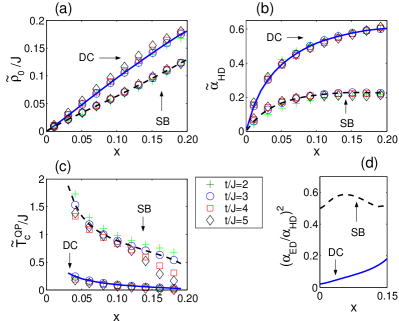
Figure 2: Doping dependence of (a) $\tilde{\rho}_{0}$, (b) $\tilde{\alpha}_{HD}$, and (c) $\widetilde{T}_{c}^{QP}$, for $t/J=2,3,4,5$ (see legend) and $t^{\prime},t^{\prime\prime}=t_{HD}^{\prime},t_{HD}^{\prime\prime}$. Results are shown for both SB and DC theories. (d) Doping dependence of $(\alpha_{ED}/\alpha_{HD})^{2}$. Full [dashed] line in (a), (b), (c), and (d) plots $t/J=3$ results in DC [SB] theory.

We now address the doping dependent behavior of $\rho_{S}(T)$ at low temperature, in both the SB and DC theories. In Figs. 2(a)-2(c) we take the hole doped regime parameters $t^{\prime},t^{\prime\prime}=t_{HD}^{\prime},t_{HD}^{\prime\prime}$, and analyze the dependence on values of $t/J$ that pertain to the physically relevant regime $2<t/J<5$. Specifically, Fig. 2(a) depicts the scaled superfluid density $\tilde{\rho}_{0}\equiv g_{\rho}(t/J)\rho_{S}(0)$, where the scaling function $g_{\rho}(t/J)=3J/t$ in the SB theory and $g_{\rho}(t/J)=1$ in the DC theory. These results show that, in the considered parameter range, the SB approach yields $\rho_{S}(0)\propto xt$ while in the DC approach $\rho_{S}(0)\approx xJ$ is almost independent of $t$. This shows that AF correlations can renormalize the SC condensate kinetic energy scale from $xt$ to $xJ$.

Fig. 2(b) depicts the scaled nodal quasiparticle current renormalization factor $\tilde{\alpha}_{HD}\equiv g_{\alpha}(t/J)\alpha_{HD}$, where $g_{\alpha}(t/J)=(3J/t)^{1/2}$ in the SB approach and $g_{\alpha}(t/J)=(t/3J)^{1/2}$ in the DC approach. We see that, even though $\alpha_{HD}$ vanishes linearly in $x$, it displays a much weaker $x$-dependence for $x\gtrsim 0.05$. To make the last statement more quantitative consider the $t/J=3$ results, for which $\alpha_{HD}(x=0.05)/\max\{\alpha_{HD}(x),0<x<0.2\}=0.73$ and $\alpha_{HD}(x=0.10)/\max\{\alpha_{HD}(x),0<x<0.2\}=0.93$ in the SB framework, and $\alpha_{HD}(x=0.05)/\max\{\alpha_{HD}(x),0<x<0.2\}=0.65$ and $\alpha_{HD}(x=0.10)/\max\{\alpha_{HD}(x),0<x<0.2\}=0.86$ in the DC framework. We remark that the above behavior appears to be a robust property of slave-particle formulations since it applies to two different slave-particle frameworks and various $t/J$ values. This state of affairs should be contrasted with the approximate $\rho_{S}(0)\propto x$ relation applicable in both theories throughout the interval $0<x<0.2$ [Fig. 2(a)]. In addition to having different doping dependences, $\rho_{S}(0)$ and $\alpha_{HD}$ also display distinct parametric dependences on $t/J$ in either slave-particle approach. Hence, the way interactions and quantum fluctuations in doped Mott insulator superconductors renormalize $\rho_{S}(0)$ differs from the way they renormalize $\alpha$ Franz and Iyengar (2006). More importantly, we show that this difference is captured by slave-particle approaches, which are often dismissed on the grounds that they imply $\alpha\sim\rho_{S}(0)$, a relation that counters experimental evidence Liang et al. (2005); Zuev et al. (2005); Broun et al. (2005). Our calculation shows that this relation only holds in the asymptotic limit $x\rightarrow 0$, where the mismatch with experiments is expected since long-range AF order develops in material compounds.

Fig. 2(b) further shows that in the hole doped cuprate regime, i.e. for $t,t^{\prime},t^{\prime\prime}=t_{HD},t_{HD}^{\prime},t_{HD}^{\prime\prime}$, $\alpha_{HD}$ is approximately a factor of $2.5$ larger in the DC theory than in the SB approach [as expected from the quasiparticle current plots in Figs. 1(a) and 1(c)]. In particular, the inclusion of AF correlations, and the consequent momentum space anisotropy, brings $\alpha_{HD}$ up to $0.5\lesssim\alpha_{HD}\lesssim 0.6$ when $0.1\lesssim x\lesssim 0.2$ and $t/J=3$, which is quantitatively consistent with experimental data Mesot et al. (1999); Chiao et al. (2000); Hawthorn et al. (2003).

The above AF correlations-driven enhancement of $\alpha_{HD}$ also renders thermally excited quasiparticles effective in reducing the superfluid stiffness in the DC theory. This effect is depicted in Fig. 2(c), which plots $\widetilde{\text{T}}_{c}^{QP}\equiv g_{T}(t/J)\text{T}_{c}^{QP}$, where $g_{T}(t/J)=t/3J$ in the SB framework and $g_{T}(t/J)=3J/t$ in the DC framework. In particular, for $t,t^{\prime},t^{\prime\prime}=t_{HD},t_{HD}^{\prime},t_{HD}^{\prime\prime}$ and $x\gtrsim 0.10$, T${}_{c}^{QP}\sim J/10$ in the DC theory, a value that is consistent with the cuprates’ T_c scale, and represents an order of magnitude improvement over the corresponding scale obtained within the SB approach.

As Fig. 1(d) illustrates, AF correlations do not enhance the nodal quasiparticle current in the electron doped regime and, in this case, the nodal current renormalization factor $\alpha_{ED}$ is much smaller than its hole doped counterpart. This fact is attested by the small DC theory value of $(\alpha_{ED}/\alpha_{HD})^{2}\sim 0.1$ in Fig. 2(d), and is consistent with electron doped cuprates’ experimental data showing a low temperature $\rho_{S}(T)$ hard to reconcile with gapless nodal excitations Alff et al. (1999); Kim et al. (2003) despite solid evidence for predominant $d_{x^{2}-y^{2}}$-wave symmetric pairing Armitage et al. (2001); Blumberg et al. (2002); Tsuei and Kirtley (2000); Chesca et al. (2003). This asymmetry between the electron and hole doped regimes is considerably larger in the DC approach than in the SB approach [Fig. 1(d)] and, therefore, our calculation suggests that the above apparent discrepancy between different experimental probes reflects the short-range AF correlations present in the strongly correlated SC state.

The results in Fig. 2 disclose specific parametric dependences of the low temperature $\rho_{S}(T)$ on intermediate values of $t/J$, which apply throughout a wide doping range. These dependences can be remarkably different in the SB and DC approaches, thus showing that they are strongly modified by the inclusion of local staggered spin correlations. For instance, the SB theory predicts that $\alpha_{HD}$ decreases upon lowering $t/J$ while the DC approach implies the opposite trend [Fig. 2(b)]. Only the DC theory result, however, correctly captures the well documented enhancement of quasiparticle features upon lowering $t/J$ – it specifically predicts that $\alpha_{HD}\propto(J/t)^{1/2}$, a parametric dependence equal to that obtained for the nodal quasiparticle spectral weight in exact numerical calculations concerning the same parameter regime Dagotto (1994). Now consider the results in Fig. 2(c), which show that the quasiparticle-driven T_c scale lowers with increasing $t/J$ in the SB approach, whereas it increases with $t/J$ once AF correlations are included in the DC theory. The latter trend seems to be more consistent with experiments though. In fact, these support that the T_c scale is, to a large extent, set by quasiparticles, and that superconductivity emerges in underdoped cuprates as a means to enhance the kinetic energy of charge carriers Anderson (1987); Molegraaf et al. (2002); Santander-Syro et al. (2004) (which is otherwise frustrated by the background staggered moment correlations). Hence, one expects T${}_{c}^{QP}$ to grow with $t/J$, as obtained in the DC framework.

IV Experimental signature of an applied supercurrent

Gauge invariance implies that, upon substituting $A_{ij}$ by the linear combination $[A_{ij}-(\phi_{j}-\phi_{i})/2]$, where $\phi_{i}$ is the order parameter’s phase, the Hamiltonians $H_{MF}^{SB}(A_{ij},\bm{a}_{ij})$ and $H_{MF}^{DC}(A_{ij},\bm{a}_{ij})$ describe the coupling between SC quasiparticles and an applied supercurrent, which can be addressed by experiments that probe single-electron physics. One such example is ARPES, which probes the single-electron energy dispersion $E_{b,\bm{k}}(A)$, and that, at least in principle, provides the means to directly measure the quasiparticle current $j_{b,\bm{k},\hat{u}}=-\tfrac{dE_{b,\bm{k}}(A)}{dA_{\hat{u}}}$. Unfortunately though, such measurements require both good energy and momentum resolution, and are most likely unfeasible in underdoped cuprates, whose low energy quasiparticle spectral features have small intensity and large widths. Alternatively, one may use STM, which has better energy resolution than ARPES. However, STM is a local probe in real space and misses a considerable amount of momentum resolved information. In addition, since STM integrates over momentum space, it is only sensitive to the second power of an applied supercurrent’s magnitude (as long as time-reversal symmetry remains unbroken). Still, as we show in what follows, STM can be used to probe certain qualitative features that derive from the underlying quasiparticle current momentum space distribution.

IV.1 Supercurrent dependence of tunneling conductance – BCS theory

We first study the supercurrent dependence of the tunneling conductance within the BCS theory. This allows us to introduce the general formal approach, as well as to estimate the (generic) order of magnitude of the effect produced by a supercurrent on the STM spectrum.

The mean-field BCS superconducting Hamiltonian

$$H_{MF}^{BCS}=\sum_{\bm{k}}c^{\dagger}_{\alpha\bm{k}}\epsilon_{\bm{k}}c_{\alpha\bm{k}}+\sum_{\bm{k}}(c_{\alpha\bm{k}}\epsilon^{\alpha\beta}\Delta_{\bm{k}}c_{\beta,-\bm{k}}+h.c)$$ (15)

where $\epsilon_{\bm{k}}$ is the normal state dispersion, $\Delta_{\bm{k}}$ is the gap function, and $\epsilon^{\alpha\beta}$ is the anti-symmetric tensor, can be rewritten as

$$H_{MF}^{BCS}=E_{0}+\sum_{\bm{k}}(E_{\bm{k}}^{BCS}+\epsilon^{a}_{\bm{k}})b^{\dagger}_{\alpha\bm{k}}b_{\alpha\bm{k}},$$ (16)

where

$$\epsilon^{s}_{\bm{k}}=\frac{1}{2}(\epsilon_{\bm{k}}+\epsilon_{-\bm{k}}^{N})\ ,\quad\epsilon^{a}_{\bm{k}}=\frac{1}{2}(\epsilon_{\bm{k}}-\epsilon_{-\bm{k}}^{N})$$

$$E_{\bm{k}}^{BCS}=\sqrt{(\epsilon^{s}_{\bm{k}})^{2}+|\Delta_{\bm{k}}|^{2}},$$ (17)

if we introduce the fermionic Nambu operators $b_{\alpha\bm{k}}$

$$c_{\uparrow\bm{k}}=u_{\bm{k}}b_{\uparrow\bm{k}}+v_{\bm{k}}b^{\dagger}_{\downarrow,-\bm{k}}\ ,\quad c_{\downarrow\bm{k}}=u_{\bm{k}}b_{\downarrow\bm{k}}-v_{\bm{k}}b^{\dagger}_{\uparrow,-\bm{k}}$$ (18)

where $u^{2}_{\bm{k}}=\tfrac{1}{2}(1+\tfrac{\epsilon^{s}_{\bm{k}}}{E_{\bm{k}}^{BCS}})$ and $v^{2}_{\bm{k}}=\tfrac{1}{2}(1-\tfrac{\epsilon^{s}_{\bm{k}}}{E_{\bm{k}}^{BCS}})$ are the BCS coherence factors. $E_{0}$ in Eq. (16) is the ground-state energy, where the ground-state $|SC\rangle$ is determined by $b_{\alpha\bm{k}}|SC\rangle=0$ if $E_{\bm{k}}+\epsilon^{a}_{\bm{k}}>0$, and by $b^{\dagger}_{\alpha\bm{k}}|SC\rangle=0$ if $E_{\bm{k}}+\epsilon^{a}_{\bm{k}}<0$.

From the above, we can obtain the density of states

$$N(\epsilon) =\int_{B.Z.}\frac{d^{2}{\bm{k}}}{(2\pi)^{2}}\delta(E_{\bm{k}}+\epsilon^{a}_{\bm{k}}-\epsilon)u^{2}_{\bm{k}}$$

$$+\int_{B.Z.}\frac{d^{2}{\bm{k}}}{(2\pi)^{2}}\delta(E_{\bm{k}}+\epsilon^{a}_{\bm{k}}+\epsilon)v^{2}_{\bm{k}}.$$ (19)

In addition, since in layered materials like the cuprates we can approximately consider that the conductance between a metal and a superconductor at a bias voltage $V$ is proportional to the total tunneling density of states $N(\epsilon)$ of the superconductor at $\epsilon=V$ BenDaniel and Duke (1967); Wei et al. (1998), we have

$$\left(\frac{dI}{dV}\right)(V) \propto\int_{B.Z.}\frac{d^{2}{\bm{k}}}{(2\pi)^{2}}f(E_{\bm{k}}+\epsilon^{a}_{\bm{k}}-V)u^{2}_{\bm{k}}$$

$$+\int_{B.Z.}\frac{d^{2}{\bm{k}}}{(2\pi)^{2}}f(E_{\bm{k}}+\epsilon^{a}_{\bm{k}}+V)v^{2}_{\bm{k}}$$ (20)

where $f(\epsilon)=\tfrac{e^{\beta\epsilon}}{(1+e^{\beta\epsilon})^{2}}$ and $\beta=\tfrac{1}{k_{B}T}$ account for the effect of thermal broadening.

We now apply the above formula to calculate the differential tunneling conductance between a metal and a simple BCS $d$-wave superconductor whose gap function is $\Delta_{\bm{k}}=2\Delta[\cos(k_{x})-\cos(k_{y})]$, and whose dispersion in the absence of a supercurrent is $\epsilon^{0}_{\bm{k}}=-2t[\cos(k_{x})+\cos(k_{y})]+\mu$. In the presence of a supercurrent $\bm{J}_{s}$ in the plane, the energy dispersion shifts in momentum space as given by $\epsilon_{\bm{k}}=\epsilon^{0}_{\bm{k}+\bm{\kappa}}$, where $\bm{\kappa}=\bm{A}$ and where the vector potential $\bm{A}$ is determined from London’s equation $\bm{J}_{s}=\rho_{S}\bm{A}$. Since the quasiparticle current is given by $\bm{j}_{\bm{k}}=-\tfrac{\partial E_{\bm{k}}(\bm{A})}{\partial\bm{A}}$, the quasiparticle current distribution in the Brillouin zone controls the above energy dispersion shift. Consequently, the change in the tunneling spectrum due to an applied supercurrent reflects the underlying quasiparticle current distribution.

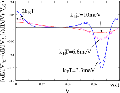
Figure 3: A plot of $\left[\left(\tfrac{dI}{dV}\right)_{\kappa}(V)-\left(\tfrac{dI}{dV}\right)_{0}(V)\right]/\left(\tfrac{dI}{dV}\right)(V_{1/2})$ as a function of bias voltage $V$ at three different temperatures and for $\kappa a=0.01$. The solid line is for electron tunneling into the superconductor and the dashed line is for electron tunneling out of the superconductor. We use $t=0.3$eV, $\mu=0.2$eV, and $\Delta=0.02$eV which results in $V_{gap}\approx 0.066$ volt. $\left(\tfrac{dI}{dV}\right)_{\kappa}(V)-\left(\tfrac{dI}{dV}\right)_{0}(V)$ has a temperature dependent peak around $V=0$. The width of the peak at the half of maximum value is about $4k_{B}T$. The height of the peak is proportional to $1/T$.

To estimate the order of magnitude of the momentum shift $\bm{\kappa}$, we consider the effect of a supercurrent density of magnitude $J_{s}=10^{8}$Amp/cm² on the surface of a superconductor. Such an current density can be achieved by passing 0.1Amp of current through a superconducting thin film of $10\mu$m wide and $0.01\mu$m thick. The penetration depth of the superconductor is $\lambda_{L}=0.1\mu$m. (Note that, here, the London penetration depth is the penetration depth for a magnetic field perpendicular to the $C_{u}O$ plane.) Since the London penetration depth $\lambda_{L}$ is given by $\lambda_{L}=\sqrt{c^{2}/4\pi\rho_{S}e^{2}}$ (the constants $e$ and $c$ are introduced for convenience), we have that

$$\bm{\kappa}=\alpha\frac{4\pi\lambda_{L}^{2}}{c}\frac{\bm{J}_{s}}{e}$$ (21)

where $\alpha$ embodies the effect of the quasiparticle current renormalization due to interactions. If we take the non-interacting case, $\alpha=1$, and we find $\kappa=1.75\times 10^{5}$/cm or $\kappa a=7\times 10^{-3}$, where $a=3.8$Å is the lattice constant of the $C_{u}O$ plane.

Let $\left(\tfrac{dI}{dV}\right)_{\kappa}(V)$ be the differential tunneling conductance in the presence of a supercurrent flowing in the $C_{u}O$ plane in the $x$-direction. [$\left(\tfrac{dI}{dV}\right)_{0}(V)$ then stands for the differential tunneling conductance in the absence of a traversing supercurrent.] Fig. 3 plots $\left[\left(\tfrac{dI}{dV}\right)_{\kappa}(V)-\left(\tfrac{dI}{dV}\right)_{0}(V)\right]/\left(\tfrac{dI}{dV}\right)(V_{1/2})$ for the choice of parameters $t=0.3$eV, $\mu=0.2$eV, $\Delta=0.02$eV, and $\kappa a=0.01$. Here we use the scale factor $\left(\tfrac{dI}{dV}\right)(V_{1/2})$, which denotes the differential tunneling conductance at $V_{1/2}=0.033\text{V}=V_{gap}/2$. Following the above calculation we expect that, in an experimentally relevant context, the change in the tunneling spectrum is of the order of $0.001-0.01$ of the original signal’s magnitude. The effect of supercurrent on the tunneling $dI/dV$ curve can also be studied by tunneling near a vortex.

IV.2 Supercurrent dependence of tunneling conductance – DC and SB theories

We now focus on the particular case of a doped Mott insulator superconductor as described by the SB and DC theories. We thus extend previous calculations of the tunneling differential conductance using the SB and DC frameworks Rantner and Wen (2000); Ribeiro and Wen (2006b) to account for the presence of an applied supercurrent. Specifically, we consider the mean-field Hamiltonians $H_{MF}^{SB}(A_{ij})\equiv H_{MF}^{SB}(A_{ij},\bm{a}_{ij})|_{\bm{a}=-\left(\bm{\Pi}_{aa}^{SB}\right)^{-1}\!\!.\,\,\bm{\Pi}_{aA}^{SB}\,A}$ and $H_{MF}^{DC}(A_{ij})\equiv H_{MF}^{DC}(A_{ij},\bm{a}_{ij})|_{\bm{a}=-\left(\bm{\Pi}_{aa}^{DC}\right)^{-1}\!\!.\,\,\bm{\Pi}_{aA}^{DC}\,A}$ to determine the dependence of the mean-field energy dispersions $E_{\bm{k}}^{SB}(\bm{A})$ and $E_{\bm{k}}^{DC}(\bm{A})$ on the gauge field $\bm{A}$. We then straightforwardly obtain the dependence of the differential tunneling conductance $\left(\tfrac{dI}{dV}\right)_{\kappa}(V)$ on $\bm{A}$ for both the SB and in the DC approaches as outlined in Sec. IV.1. Let we, however, note a few technical differences between what follows and Sec. IV.1. Firstly, below we assume that interactions provide the main contribution to the broadening of spectral features of doped Mott insulators. Hence, instead of thermal broadening, we include the effect of a Lorentzian broadening parameterized by $\Gamma=0.01t$ (a value consistent with experiments Oda et al. (1997); Howald et al. (2001)). Secondly, we explicitly focus on the small $\kappa$ limit, in which case we can write

$$\left(\frac{dI}{dV}\right)_{\kappa}\!\!\!(V)=\left(\frac{dI}{dV}\right)_{0}\!\!\!(V)+\frac{\kappa^{2}}{2}\left(\frac{dI}{dV}\right)^{\prime\prime}\!\!\!(V)+O(\kappa^{4})$$ (22)

since in the absence of time-revesal symmetry breaking $\left(\tfrac{dI}{dV}\right)_{\kappa}(V)=\left(\tfrac{dI}{dV}\right)_{-\kappa}(V)$. Hence, below, we focus on the behavior of $\left(\tfrac{dI}{dV}\right)^{\prime\prime}(V)$ instead of selecting a particular value of $\kappa$.

Figs. 4(a) and 4(b) depict the resulting DC and SB theory plots of

$$\left(\frac{dI}{dV}\right)_{norm}^{\prime\prime}\!\!\!\!\!\!\!\!\!(V)\ \equiv\ \left(\frac{dI}{dV}\right)^{\prime\prime}\!\!\!(V)\,/\left(\frac{dI}{dV}\right)^{\prime\prime}\!\!\!(0)$$ (23)

for $x=0.05$ and $x=0.15$ and in the subgap frequency range $-V_{gap}/2<V<V_{gap}/2$, where $V$ is the bias voltage and $V_{gap}$ is the SC coherence peak voltage. (We only show results for the above values of $V$ in order to focus on the specific experimental signature we discuss below.) In the above expression we normalize the second derivative of the tunneling conductance with respect to $\kappa$ so that it equals unity at $V=0$.

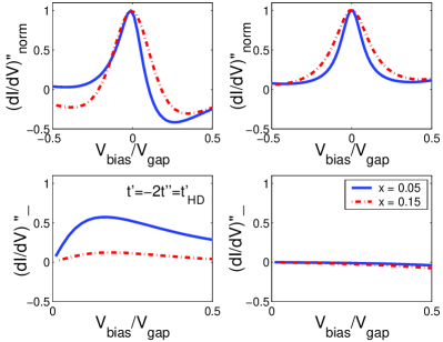
Figure 4: (a) $(\tfrac{dI}{dV})_{norm}^{\prime\prime}$ in DC theory. (b) $(\tfrac{dI}{dV})_{norm}^{\prime\prime}$ in SB theory. (c) $(\tfrac{dI}{dV})_{-}^{\prime\prime}$ in DC theory. (d) $(\tfrac{dI}{dV})_{-}^{\prime\prime}$ in SB theory. We plot the $x=0.05$ (full line) and $x=0.15$ (dashed line) results for $t,t^{\prime},t^{\prime\prime}=t_{HD},t_{HD}^{\prime},t_{HD}^{\prime\prime}$, and use a Lorentzian broadening given by $\Gamma=0.01t$. A finite $\Gamma$ corresponds to a finite effetive temperature $T$ whose value is propotional to and can be estimated from the width of the peak at $V=0$. The width at the half peak value is about $4k_{B}T$ (see Fig. 3).

The interesting feature in Figs. 4(a) and 4(b) is that, out of all the curves in these two figures, the DC theory plot of $(\tfrac{dI}{dV})_{norm}^{\prime\prime}$ for $x=0.05$ stands out as the only curve which is clearly asymmetric around $V=0$. To further emphasize the asymmetry in the DC theory $x=0.05$ curve, as well as the symmetry around $V=0$ of all other curves, in Figs. 4(c) and 4(d) we plot $(\tfrac{dI}{dV})_{-}^{\prime\prime}$, where

$$\left(\frac{dI}{dV}\right)_{-}^{\prime\prime}\!\!\!(V)\ \equiv\ \left(\frac{dI}{dV}\right)_{norm}^{\prime\prime}\!\!\!\!\!\!\!\!\!(-V)-\left(\frac{dI}{dV}\right)_{norm}^{\prime\prime}\!\!\!\!\!\!\!\!\!(V).$$ (24)

The question then arises of what the physical reason that singles out the DC theory $x=0.05$ curve is. We find there are at least three reasons to associate the tilting toward the negative bias side in the DC theory $x=0.05$ curve to the presence of local staggered moment correlations. Firstly, such a qualitative feature is altogether absent in the SB results. Secondly, the above asymmetry develops upon lowering $x$, which is known to enhance the signatures of AF correlations. Lastly, it naturally follows from the DC theory two-band picture that describes the interplay between coexisting AF and SC correlations at short length scales Ribeiro and Wen (2005, 2006a). To clarify the latter point, we remark that the DC mean-field theory contains two different families of fermions, namely spinons and dopons, whose dispersions are determined by Eqs. (9) and (10). Applying a supercurrent shifts the spinon and dopon bands relatively to each other and, thus, affects the electronic spectral weight transfer to low energy [which is determined by the hybridization of spinons and dopons described in Eq. (11)]. This spectral weight transfer is reduced mainly in those regions of momentum space where the second derivative with respect to momentum of the energy difference between both bands is larger, which happens to occur close to the peak of the AF-like dopon dispersion, hence close to $(\pi/2,\pi/2)$. Since the spinon nodal point shifts away from $(\pi/2,\pi/2)$ toward $(0,0)$, the above spectral weight reduction is stronger in the positive bias side, as obtained in Fig. 4(a) [this argument implies that if the nodal point were to shift toward $(\pi,\pi)$, the $(\tfrac{dI}{dV})^{\prime\prime}$ curve would rather tilt in the opposite direction].

From the above argument, the DC theory bias asymmetry in $(\tfrac{dI}{dV})^{\prime\prime}$ relies on two things, namely, the nodal point shift away from $(\pi/2,\pi/2)$ and the presence of strong local AF correlations. There exists ample experimental evidence for the former Ding et al. (1997); Zhou et al. (2004); Ino et al. (2002); Shen et al. (2004). As to the latter, AF correlations were proposed to underlie the momentum space anisotropy that weakens the differential tunneling conductance SC coherence peaks Ribeiro and Wen (2006b). Therefore, we propose that if, indeed, local AF correlations are the cause of the aforementioned differentiation of the nodal and antinodal momentum space regions, an asymmetry around $V=0$ should be detected in the $(\tfrac{dI}{dV})^{\prime\prime}$ curve measured by STM experiments in the large gap (and small coherence peak) regions of inhomogeneous BSCCO samples traversed by a supercurrent. This effect should be weaker, if at all observable, in the small gap (and large coherence peak) regions of these same samples.

We remark that the above asymmetry in $(\tfrac{dI}{dV})^{\prime\prime}$ is maximal at low values of $V$ (in the above calculation, this asymmetry peaks around $V\approx 0.15V_{gap}$). At this energy scale the differential conductance in the absence of a supercurrent, namely $\left(\tfrac{dI}{dV}\right)_{0}(V)$, is nearly symmetric around $V=0$, which should facilitate the detection of the aforementioned low energy bias asymmetry. The low bias tunneling spectrum is also nearly spatially homogeneous, a fact that should also facilitate the detection of the spatially inhomogeneous asymmetry of $(\tfrac{dI}{dV})^{\prime\prime}$ at low bias. In this context, we find that, within the DC framework, the low bias $(\tfrac{dI}{dV})^{\prime\prime}$ spatial inhomogeneity correlates with three aspects of the differential tunneling conductance at higher energy, namely, the gap size, the size of SC coherence peaks, and the high energy asymmetry between positive and negative bias.

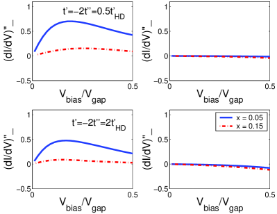
Figure 5: $(\tfrac{dI}{dV})_{-}^{\prime\prime}$ for $t,t^{\prime},t^{\prime\prime}=t_{HD},0.5t_{HD}^{\prime},0.5t_{HD}^{\prime\prime}$ in: (a) DC theory and (b) SB theory. $(\tfrac{dI}{dV})_{-}^{\prime\prime}$ for $t,t^{\prime},t^{\prime\prime}=t_{HD},2t_{HD}^{\prime},2t_{HD}^{\prime\prime}$ in: (c) DC theory and (d) SB theory. We plot the $x=0.05$ (full line) and $x=0.15$ (dashed line) results and use a Lorentzian broadening given by $\Gamma=0.01t$.

The above proposal of a specific experimental signature of a traversing supercurrent in the STM spectra of BSCCO samples relies on a calculation that assumes an homogeneous system. There are two reasons to believe our proposal is robust to the BSCCO samples’ spatial inhomogeneity. Firstly, the large BSCCO’s STM spectral diversity can be reproduced in homogeneous systems proximate to a Mott insulator transition Ribeiro and Wen (2006b). Secondly, the spatial inhomogeneity correlates with off-plane disorder McElroy et al. (2005) which affects the effective parameters $t^{\prime}$ and $t^{\prime\prime}$, but not $t$ and $J$ Pavarini et al. (2001). In Fig. 5 we depict the DC and SB theory results for the curves $(\tfrac{dI}{dV})_{-}^{\prime\prime}$ with $x=0.05$ and $x=0.15$, as well as $t^{\prime}=-2t^{\prime\prime}=0.5t_{HD}^{\prime}$ and $t^{\prime}=-2t^{\prime\prime}=2t_{HD}^{\prime}$. These show that our $(\tfrac{dI}{dV})_{-}^{\prime\prime}$ results are almost insensitive to changes in $t^{\prime}$ and $t^{\prime\prime}$ in the range $2t_{HD}^{\prime}<t^{\prime}<0.5t_{HD}^{\prime}$ and $0.5t_{HD}^{\prime\prime}<t^{\prime\prime}<2t_{HD}^{\prime\prime}$, which argues in favor of the robustness of the experimental effects discussed above.

V Summary

As discussed in the introduction, experimental data together with theoretical arguments support the important role of thermally excited SC quasiparticles in setting the T_c scale of underdoped cuprates. In this paper, we use two different wave functions, namely the SB Wen and Lee (1996); Lee et al. (1998) and DC Ribeiro and Wen (2005, 2006a) $d$-wave SC wave functions, together with the $tt^{\prime}t^{\prime\prime}J$ model Hamiltonian, to show that the combined effect of slave-particles and local AF correlations reproduces non-trivial aspects of these quasiparticles’ low energy and long wavelength electromagnetic response.

Slave-particle formulations are attractive in that they provide a microscopic description of doped Mott insulator superconductors which yields both (i) a non-vanishing quasiparticle $d$-wave gap and (ii) a vanishing effective density of charge carriers as the half-filling composition is approached. However, previous work on the SC electromagnetic response in slave-particle frameworks Lee (2000) was not consistent with a third crucial experimental fact, namely, that the nodal current renormalization factor $\alpha$ displays a much weaker $x$-dependence than $\rho_{S}(0)$. The aforementioned work was concerned with the $x\rightarrow 0$ limit, where real materials display long-range AF order and do not superconduct. Even though variational Monte-Carlo studies have extended the calculation of $\alpha$ to doping values beyond the above limit Nave et al. (2006), this technique only obtains a maximum bound on the value of $\rho_{S}(0)$ Paramekanti et al. (2004). In this paper, we relax the no-double occupancy constraint (which is implemented exactly in the variational Monte-Carlo approach) and only include (the gapped) gauge fluctuations at the Gaussian level. This allows us to calculate the temperature dependent electromagnetic response in the static and uniform limit for two different slave-particle approaches and, consequently, we are able to compare the doping dependence and the $t/J$ parametric dependence of both $\rho_{S}(0)$ and $\alpha$. Interestingly, we find that, even though $\alpha\sim\rho_{S}(0)\sim x$ in the limit $x\rightarrow 0$, away from this limit $\alpha$ is much more weakly $x$-dependent than $\rho_{S}(0)$. This result applies to both utilized slave-particle frameworks and, we propose, may be generic to slave-particle formulations.

In this paper, we also compare the SB and the DC theory results to learn how high energy and short-range staggered moment correlations affect the SC electromagnetic response in the static and uniform limit. We find that inclusion of these correlations improves SB results, as we summarize below. For instance, the SB and the DC theories imply different parametric dependences on intermediate $t/J$ values and, in Sec. III.2, we argue in favor of the DC theory expectations. We also find that local AF correlations, which enhance the quasiparticle current in specific momentum space regions that differ for the hole and electron doped regimes, provide a microscopic rationale for the experimentally observed hole vs. electron doped asymmetry in the nodal quasiparticles’ electromagnetic response. The aforementioned quasiparticle current renormalization further brings quantitative agreement with hole doped cuprates’ experimental data, specifically $\alpha$ and the T_c scale for $x\gtrsim 0.10$, if we use physically relevant bare parameters in the $tt^{\prime}t^{\prime\prime}J$ model Hamiltonian. To understand the above improvement upon inclusion of AF correlations note that, in the SB framework, the projection constraint is implemented after integrating out the $SU(2)$ gauge field, a procedure that enhances this type of AF correlations Rantner and Wen (2002). To check the consistency of this interpretation, we refer to a variational Monte-Carlo study Nave et al. (2006) that exactly enforces the no-double occupancy constraint on BCS wave functions and whose values of $\alpha$ are indeed larger than those we obtain in this paper’s SB approach.

Finally, we point out that a momentum dependent, and thus energy dependent, coupling of quasiparticles to an electromagnetic gauge field is reflected in the local density of states in the presence of an applied supercurrent. In this context, we derive (DC theory specific) qualitative predictions for the effect of short-range staggered correlations between local moments in the tunneling spectrum of a sample traversed by a supercurrent, namely, this theory implies an asymmetry in $(\tfrac{dI}{dV})^{\prime\prime}(V)$ around $V=0$ for underdoped samples. This effect may be probed by STM experiments, which thus could distinguish the DC theory description of the high-T_c superconductors from the SB theory and the conventional BCS theory.