Conductivity of a superlattice with parabolic miniband

Abstract

The static and high-frequency differential conductivity of a one-dimensional superlattice with parabolic miniband, in which the dispersion law is assumed to be parabolic up to the Brillouin zone edge, are investigated theoretically. Unlike the earlier published works, devoted to this problem, the novel formula for the static current density contains temperature dependence, which leads to the current maximum shift to the low field side with increasing temperature.

The high-frequency differential conductivity response properties including the temperature dependence is examined and opportunities of creating a terahertz oscillator on Bloch electron oscillations in such superlattices are discussed.

Analysis shows that superlattices with parabolic miniband dispersion law may be used for generation and amplification of terahertz fields only at very low temperatures ($T\to 0$).

1 Introduction

In present work, we study theoretically the static and high-frequency conductivity of a semiconductor superlattice (SL). Unlike the earlier published numerous works, devoted to this problem, where the conventional cosine-type model was used for the conduction miniband, here a dispersion law is considered in form of a truncated parabola, i. e. the dispersion law is assumed to be parabolic up to the Brillouin zone edge. Such a problem statement is of interest, among others, from the view point of opportunities of creating a terahertz oscillator on Bloch electron oscillations in SLs. In works [1]-[4] different variants of realization of such opportunity were discussed and it was mentioned that the main obstacle consists in using the non-optimal SL structures, in particular, the SL with cosine-type miniband.

Thus the theoretical investigations of electric properties of SLs with other dispersion laws are necessary, all the more so since the modern technology allows to vary widely the form of the potential relief and the SL energy spectrum.

The main condition for realization of Bloch oscillator consists in existence of negative high-frequency differential conductivity on that regions of current-voltage characteristic where the static differential conductivity is positive. In [2] it was shown that this condition holds, in particular, in SL with parabolic miniband. But this result was obtained in the limiting case $T\to 0$. Here we find the temperature dependence of conductivity of such SL and define the temperature criterion by which the mentioned condition holds practically.

This article is structured as follows. In Section 2 we derive an expression for static conductivity of SL with parabolic miniband, which is valid for any temperatures. In Section 3 we derive the corresponding expression for high-frequency differential conductivity. Section 4 presents the conclusions of our work.

2 Static distribution function and current-voltage characteristic

The electron energy in the SL lowest miniband is [1]

$$\varepsilon(\mathbf{p})=\varepsilon(\mathbf{p}_{\bot})+\frac{p^{2}}{2m},\quad-\frac{\pi\hbar}{d}<p<\frac{\pi\hbar}{d},$$ (1)

where $\mathbf{p}$ is quasimomentum, $d$ is SL period, $x$ axis being directed along the SL axis, $\varepsilon(\mathbf{p}_{\bot})$ is in-plane electron energy, $\pi^{2}\hbar^{2}/md^{2}\equiv\Delta$ is double miniband width, $m$ is effective electron mass.

In quasi-classical situation ($\Delta\gg eEd,\,\hbar/\tau$, where $\tau$ is electron momentum relaxation time, $e$ is electron charge), the current density in electric field $\mathbf{E}^{tot}(t)$ may be found by solving Boltzmann equation with collision integral within $\tau$-approximation:

$$\frac{\partial F(\mathbf{p},t)}{\partial t}+\left(e\mathbf{E}^{tot}(t),\frac{\partial F(\mathbf{p},t)}{\partial\mathbf{p}}\right)=\frac{F_{0}(\mathbf{p})-F(\mathbf{p},t)}{\tau},$$ (2)

where $F_{0}(\mathbf{p})$ is equilibrium electron distribution function, $F(\mathbf{p},t)$ is unknown distribution function perturbed due the electric field. Below we use dimensionless variables by changing $\mathbf{p}d/(\pi\hbar)\rightarrow\mathbf{p}$, $\mathbf{E}^{tot}ed\tau/(\pi\hbar)\rightarrow\mathbf{E}^{tot}$, $T/\Delta\rightarrow T$, $t/\tau\rightarrow t$ ($T$ is temperature in energy units).

With the field $\mathbf{E}^{tot}(t)$ is directed along the SL axis $\left(\mathbf{E}^{tot}(t)=\left(E^{tot}(t),0,0\right)\right)$, we have $F(\mathbf{p},t)=f_{0}(\mathbf{p}_{\bot})f(p,t)$, $F_{0}(\mathbf{p})=f_{0}(\mathbf{p}_{\bot})f_{0}(p)$, where $f_{0}(p)$ is equilibrium distribution function, normalized to the carrier density $n$ ($f_{0}(\mathbf{p}_{\bot})$ being normalized to unity). Thus, the function $f(p,t)$ satisfies the following equation

$$\frac{\partial f(p,t)}{\partial t}+E^{tot}(t)\frac{\partial f(p,t)}{\partial p}=f_{0}(p)-f(p,t),\quad(-1<p<1).$$ (3)

with periodicity conditions $f(1,t)=f(-1,t)$.

In a static field $E^{tot}(t)=E=const$, and denoting $f(p)=f_{c}(p,E,T)$, we get

$$E\frac{{\rm d}f_{c}}{{\rm d}p}=f_{0}-f_{c},\quad(-1<p<1).$$ (4)

We consider non-degenerate electron gas, so that

$$f_{0}(p,T)=2n\left[\sqrt{2\pi T}\mathrm{erf}\left(\frac{1}{\sqrt{2T}}\right)\right]^{-1}\exp\left(-\frac{p^{2}}{2T}\right)$$ (5)

where $\mathrm{erf}(z)$ is error function. In the low temperature limit ($T\rightarrow 0$) the relation (5) reduces to the function used in [1]: $g_{0}(p)=2n\delta(p)$.

The exact solution of (4) with periodicity condition, $f_{c}(-1)=f_{c}(1)$, takes the form [5]

$$f_{c}(p,E,T)=\frac{n}{E\mathrm{erf}\left(1/\sqrt{2T}\right)}\exp\left(\frac{T}{2E^{2}}-\frac{p}{E}\right)\left\{\mathrm{erf}\left(\frac{p}{\sqrt{2T}}-\frac{\sqrt{T}}{\sqrt{2}E}\right)\right.$$

$$-\left[\exp\left(\frac{2}{E}\right)-1\right]^{-1}\mathrm{erf}\left(\frac{\sqrt{T}}{\sqrt{2}E}-\frac{1}{\sqrt{2T}}\right)$$

$$+\left.\left[1-\exp\left(-\frac{2}{E}\right)\right]^{-1}\mathrm{erf}\left(\frac{\sqrt{T}}{\sqrt{2}E}+\frac{1}{\sqrt{2T}}\right)\right\},\quad-1<p<1.$$ (6)

In limiting case $E\rightarrow 0$ (6) reduces to (5). In another limiting case, $T\rightarrow 0$, we get the distribution function found in [1]:

$$g(p,E)=\frac{2n}{E}\exp\left(-\frac{p}{E}\right)\cases{[1-\exp(-2/E)]^{-1},&$0<p<1$,\cr[\exp(2/E)-1]^{-1},&$-1<p<0$}.$$ (7)

The function (6) satisfies the same normalization condition as the equilibrium function $f_{0}$

$$\frac{1}{2}\int\limits_{-1}^{1}f_{c}(p,E,T)\,dp=n$$ (8)

and, therefore, it makes the integral of right-hand side of formula (4) vanish. Besides, the integral of left-hand side of the Boltzmann equation (4) vanishes too, because of the periodicity condition mentioned. The distribution function $f_{c}(p,E,T)$ at several values of $E$ and $T$ is shown in figure 1.

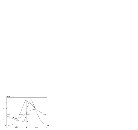
Figure 1: Distribution function $f_{c}(p)$ at various values of the driving field and temperature. 1) $E=1,\;T=0.1$; 2) $E=0.1,\;T=0.1$; 3) $E=2,\;T=2$; 4) $E=1,\;T=0.005$. The dashed curve 5 represents function $g(p)$ at $E=1$.

The current density $j$ in the direction of SL axis can be found (in dimensional units) by a conventional way

$$j=\frac{ed}{2\pi\hbar m}\int\limits_{-\pi\hbar/d}^{\pi\hbar/d}pf_{c}(p)\,dp.$$ (9)

By substitution function (6) into (9) we get

$$j(E,T)=E+\left[2\mathrm{erf}\left(\frac{1}{\sqrt{2T}}\right)\sinh\left(\frac{1}{E}\right)\right]^{-1}\exp\left(\frac{T}{2E^{2}}\right)$$

$$\times\left[\mathrm{erf}\left(\frac{\sqrt{T}}{E\sqrt{2}}-\frac{1}{\sqrt{2T}}\right)-\mathrm{erf}\left(\frac{\sqrt{T}}{E\sqrt{2}}+\frac{1}{\sqrt{2T}}\right)\right].$$ (10)

Here $j$ is expressed in units of $j_{0}=ne\Delta d/\pi\hbar$, while all the quantities are written in dimensionless form.

Equation (10) determines the current-voltage characteristic for the parabolic miniband SL with the current density temperature dependence taking into account.

To warrant numerical stability we present formula (10) in the following form

$$j(E,T)=E\sigma(E,T),\quad\sigma(E,T)=1-\sqrt{\frac{2}{\pi T}}\frac{\exp(-0.5/T)+A(E,T)}{\mathrm{erf}(1/\sqrt{2T})},$$ (11)

where $\sigma(E,T)$ is the conductivity and

$$A(E,T)=\frac{E^{2}}{T\sinh(1/E)}\int\limits_{0}^{1/E}\exp\left(-\frac{s^{2}E^{2}}{2T}\right)s\sinh s\,ds.$$ (12)

The value of $A(E,T)$ can be estimated numerically with high accuracy.

Expanding the exponent in a power series we get

$$A(E,T)=\frac{1}{T}\sum_{n=0}^{\infty}\frac{(-1)^{n}}{(2n)!!}\frac{G_{n}(E)}{T^{n}},$$ (13)

where functions $G_{n}(E)$ are defined by recurrent formula

$$G_{0}=E\coth\left(\frac{1}{E}\right)-E^{2},\quad G_{n}=G_{0}+2nE^{2}\left[(2n+1)G_{n-1}-1\right].$$ (14)

As $G_{n}(E)\in[0,1/(2n+3))$, series (13) converges quickly. As numerical experiments show, first four terms of series (13) give good approximation at $T>0.5$.

At $|E|\to 0$ we have $A(E,T)\to 0$, so in low fields ($|E|\ll 1$) in linear approximation on $E$ we have

$$j(E,T)=E\left(1-\sqrt{\frac{2}{\pi T}}\frac{\exp(-0.5/T)}{\mathrm{erf}(1/\sqrt{2T})}\right)=E\left\langle\frac{p^{2}}{T}\right\rangle_{0},$$ (15)

where angle brackets mean averaging over the equilibrium distribution. Note that the conductivity temperature dependence in low fields (the expression within round brackets in (15)) is close to the analogous dependence for the miniband cosine model ($I_{1}(1/2T)/I_{0}(1/2T)$, $I_{n}(z)$ being the modified Bessel function).

In high fields ($|E|>1$) we have

$$\sigma(E,T)\approx\frac{\sqrt{2/\pi}}{E^{2}T\sqrt{T}\mathrm{erf}(1/\sqrt{2T})}\sum_{n=0}^{\infty}\frac{(-1)^{n+1}}{(2n)!!}\frac{D_{n}}{T^{n}},\quad D_{n}=\sum_{k=2}^{n+2}\frac{2^{2k}(2n+1)!B_{2k}}{(2k)!(2n-2k+5)!},$$ (16)

where $B_{m}$ are Bernoulli numbers.

For low temperatures ($T\ll 1$), using (12), we get

$$\sigma(E,T)\approx 1-\frac{1}{\mathrm{erf}\left(1/\sqrt{2T}\right)}\left[\frac{1}{E\sinh(1/E)}\exp\left(\frac{T}{2E^{2}}\right)+\sqrt{\frac{2}{\pi T}}\exp\left(-\frac{1}{2T}\right)\right].$$ (17)

As numerical experiments show, formula (17) gives good approximation at $T<0.07$. In limiting case $T\to 0$ from (17) we get the expression that was found in [1]

$$j=j(E)=E-\frac{1}{\sinh(1/E)}.$$ (18)

From (15,16) it follows that $j\sim E$ at $|E|\ll 1$ and $j\sim 1/E$ at $|E|\gg 1$. Therefore at fixed temperature $T=fix$ the function $j(E,T)$ reaches its maximum at some value $E=E_{C}(T)>0$ and negative differential conductivity is realized at $E>E_{C}(T)$ (see figure 2).

Figure 2: Current-voltage characteristic at different values of temperature. 1) $T=0$; 2) $T=0.01$; 3) $T=0.1$; 4) $T=0.5$; 5) $T=1$.

Note, that $E_{C}(T)$ decreases with increasing temperature. Essentially, that $E_{C}$ value does not depend on the temperature at all in the cosine model: $E_{C}=1/\pi\approx 0.318$.

The parametric representation of dependence $E_{C}(T)$ is defined by equation $\sigma_{d}=0$, where $\sigma_{d}=\partial j/\partial E$ is the differential conductivity. Using (11,12), we get

$$\sigma_{d}(E,T)= 1+\frac{1}{E^{2}}\left\{\left[E\coth\left(\frac{1}{E}\right)-T\right]\left[\sigma(E,T)-1\right]\right.-$$ (19)

$$\left.\sqrt{\frac{2T}{\pi}}\frac{1}{\mathrm{erf}\left(1/\sqrt{2T}\right)}\exp\left(-\frac{1}{2T}\right)\right\},$$

Thus function $E_{C}(T)$ is defined implicitly by equation

$$E^{2}\sqrt{\frac{\pi T}{2}}\mathrm{erf}\left(\frac{1}{\sqrt{2T}}\right)+TA(E,T)=E\coth\left(\frac{1}{E}\right)\left[A(E,T)+\exp\left(-\frac{1}{2T}\right)\right],$$ (20)

and it is sufficient to solve this equation at $E>0$.

The numerical solution of equation (20) at $E$ versus $T$ is presented in figure 3.

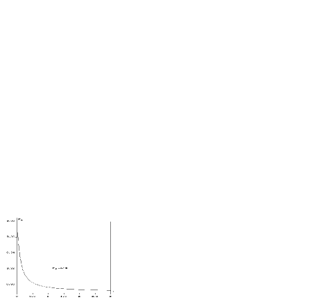
Figure 3: The dependence $E=E_{C}(T)$. The dashed curve $E_{C}=1/\pi$ represents $E_{C}$ for cosine model.

Note that dependence $E=E_{C}(T)$ is monotone so the inverse function $T_{C}=T_{C}(E)$ exists. To investigate behavior of function $T_{C}(E)$, consider first the case of high temperatures $T\gg 1$. Expanding all functions in a power series on $1/T$ and neglecting all terms $o(1/T^{2})$, we get

$$T_{C}\approx\frac{(45E^{4}+22.5E^{2}+1.8)\tanh^{2}\left(1/E\right)-(36E+3E)\tanh\left(1/E\right)-9E^{2}-1.5}{(9E^{2}+4)\tanh^{2}\left(1/E\right)-6E\tanh\left(1/E\right)-3}$$ (21)

By that

$$\lim_{E\to E_{1}+0}T_{C}(E)=+\infty,$$ (22)

where $E_{1}\approx 0.29104955$ is the root of equation

$$(9E^{2}+4)\tanh^{2}\left(\frac{1}{E}\right)-6E\tanh\left(\frac{1}{E}\right)-3=0.$$ (23)

Consider now the case of low temperatures $T\ll 1$. Using (17), we get

$$T_{C}(E)\approx 2E^{2}\left[E^{2}\tanh\left(\frac{1}{E}\right)\sinh\left(\frac{1}{E}\right)-1\right]\left[1-2E\tanh\left(\frac{1}{E}\right)\right]^{-1}.$$ (24)

By that

$$\lim_{E\to E_{2}-0}T_{C}(E)=0,$$ (25)

where $E_{2}\approx 0.373681745$ is the root of equation

$$E^{2}\tanh\left(\frac{1}{E}\right)\sinh\left(\frac{1}{E}\right)=1.$$ (26)

Therefore function $E_{C}(T)$ is defined for $T>0$ and

$$\lim_{T\to 0}E_{C}(T)=E_{2},\quad\lim_{T\to+\infty}E_{C}(T)=E_{1}.$$ (27)

3 High-frequency differential conductivity

In this section we will determine the induced superlattice current in the presence of an external electric field given by

$$E^{tot}(t)=E+E_{0}\cos\omega t,$$ (28)

where $\omega$ is measured in units of $\tau^{-1}$. Within the scope of quasi-classical conditions the value of $E$ is arbitrary. Assuming the amplitude of variable field $E_{0}$ to be much smaller then the static field $E$, consider the time-dependent field in linear approximation. The distribution function may be found in a form

$$f(p,E,T,t)=f_{c}(p,E,T)+f_{1}(p,E,T,\omega)\exp(-i\omega t),$$ (29)

here $f_{1}(p,E,\omega)$ satisfies the following equation [2]

$$E\frac{\partial f_{1}}{\partial p}+(1-i\omega)f_{1}=-E_{0}\frac{\partial f_{c}}{\partial p}$$ (30)

with periodicity condition $f_{1}(-1,E,\omega)=f_{1}(1,E,\omega)$ and by

$$\int_{-1}^{1}f_{1}(p,E,T,\omega)\,dp=0.$$ (31)

It is easily to show that required solution is

$$f_{1}(p,E,T,\omega)=\frac{i}{\omega}\cdot\frac{E_{0}}{E}\left[f_{c}(p,E,T)+f_{c}\left(p,\frac{E}{1-i\omega}\right),T\right].$$ (32)

With the help of (32) the dynamic (high-frequency) differential conductivity can be found by a conventional way. The result is

$$\sigma_{1}(E,T,\omega)=\frac{i}{\omega E}\left[j(E,T)-j\left(\frac{E}{1-i\omega},T\right)\right].$$ (33)

From (33) it follows that at $\omega\to 0$ the value $\sigma_{1}(E,T,\omega)$ tends to static differential conductivity (19)

$$\lim_{\omega\to 0}\sigma_{1}(E,T,\omega)=\sigma_{d}(E,T).$$ (34)

Using (10), we get

$${{Re}}\,\sigma_{1}(E,T,\omega)=\frac{i}{2\omega E}\left[j\left(\frac{E}{1+i\omega},T\right)-j\left(\frac{E}{1-i\omega},T\right)\right].$$ (35)

For numerical computations we present expression (35) in a form

$${{Re}}\,\sigma_{1}(E,T,\omega)=\frac{1}{1+\omega^{2}}$$

$$-\sqrt{\frac{2}{\pi T}}\frac{\left[\sinh^{2}(1/E)+\sin^{2}(\omega/E)\right]^{-1}}{\omega E\mathrm{erf}\left(1/\sqrt{2T}\right)}\left[\cosh\frac{1}{E}\sin\frac{\omega}{E}\int_{0}^{1}\exp\left(-\frac{s^{2}}{2T}\right)\cosh\frac{s}{E}\cos\frac{s\omega}{E}\,ds\right.$$

$$-\left.\sinh\frac{1}{E}\cos\frac{\omega}{E}\int_{0}^{1}\exp\left(-\frac{s^{2}}{2T}\right)\sinh\frac{s}{E}\sin\frac{s\omega}{E}\,ds\right].$$ (36)

At $T\to 0$ from (36) we get the expression presented in [2]

$${{Re}}\,\sigma_{1}(E,0,\omega)=\frac{1}{1+\omega^{2}}-\frac{\cosh(1/E)\sin(\omega/E)}{\omega E\left[\sinh^{2}(1/E)+\sin^{2}(\omega/E)\right]}$$ (37)

The opportunities of creating a terahertz oscillator on Bloch electron oscillations in SLs are defined by conditions of existence of negative high-frequency differential conductivity on that regions of current-voltage characteristic where the static differential conductivity is positive [2]-[4]. These conditions would prevent development of undesirable domain instabilities (Gunn effect).

Let $\Omega=eEd/\hbar$ be the Bloch oscillations frequency which in normalized measurement units is equal to $\pi E$. Then the static differential conductivity $\sigma_{d}$ is positive at $\Omega<\Omega_{C}$ and negative at $\Omega>\Omega_{C}$, where $\Omega_{C}=\pi E_{C}(T)\in(0.914,1.174)$. Thus the conditions of low-frequency domain instability suppression are defined by that values of parameters $\omega$ and $\Omega$, for which

$$\cases{\Omega<\Omega_{C}\cr\sigma_{1}(\Omega,T,\omega)<0}$$ (38)

The existence of such conditions for regarded model of dispersion law was discovered in [2] in limiting case $T\to 0$.

But conditions (38) prove to be very sensitive to temperature increasing. In figure 4 the regions in parameter space $(\Omega,T,\omega)$ are presented in which the high-frequency differential conductivity is negative.

Figure 4: The regions of negative high-frequency differential conductivity at parameter plane $(\Omega,\omega)$. a) $T\to 0$, $\Omega_{C}=1.174$. b) $T=0.01$, $\Omega_{C}=1.06$.

The boundary lines of these regions are defined by condition ${{Re}}\,\sigma_{1}(E,T,\omega)=0$. At these lines we have $\omega\approx k\Omega$, $k=1,2,\dots$. Thus the frequencies at which the high-frequency differential conductivity changes sign are multiples of the Bloch frequency.

Note the existence of regions of low-frequency domain instability suppression at $T=0$ and absence of such regions at $T=0.01$.

The dependence of function $\sigma_{1}$ on parameters $\Omega$ and $\omega$ is presented in figure 5.

Figure 5: a) Driving field dependence of high-frequency differential conductivity at $\omega=10$. 1) $T=0$, $\Omega_{C}=1.174$; 2) $T=0.01$, $\Omega_{C}=1.163$; 3) $T=0.1$, $\Omega_{C}=1.06$. b) Dependence of high-frequency differential conductivity on $\omega$ at $\Omega=1$. 1) $T=0$; 2) $T=0.01$; 3) $T=0.1$. At such temperatures the static differential conductivity $\sigma_{d}=\left.\sigma_{1}\right|_{\omega=0}$ is positive.

Note that by temperature increasing the oscillations of $\sigma_{1}$ become suppressed at $\Omega<\Omega_{c}$ and negative high-frequency differential conductivity disappears.

4 Conclusion

In present paper, an exact distribution function has been found of the carriers in the lowest parabolic miniband of a SL, placed in the dc electric field, parallel to SL axis. The novel formula for the static current density in SL contains temperature dependence, which leads to the current maximum shift to the low field side with increasing temperature.

We have obtained explicit expression for high-frequency differential conductivity at arbitrary temperature. It was shown that high-frequency differential conductivity is very sensitive to temperature of SL. We have compared high-frequency electron behavior at different temperatures and exhibited the drastic change in the character of regions where the high-frequency differential conductivity is negative. In particular we have discovered that the possibility of low-frequency domain instability suppression may be realized only at $T\to 0$.

In summary, our analysis shows that SLs with parabolic miniband dispersion law may be used for generation and amplification of terahertz fields only at very low temperatures ($T<0.01\Delta$).

The numerical estimations of the effects predicted are reduced, in general, to measurement units of electric field and temperature. At $d=10^{-7}$ cm, $\tau=10^{-12}$ s, $\Delta\approx 10^{-2}$ eV we get that units for $E$ and $T$ are $\approx 2\cdot 10^{3}$ and $\approx 100$ K respectively. Thus the condition $T<0.01\Delta$ is equivalent to $T<1$ K.

References

References

• [1] Romanov Yu A 2003 Phys. Solid State 45 559
• [2] Romanov Yu A, Mourokh L G and Horing N J M 2002 cond-mat/0209365
• [3] Romanov Yu A and Romanova J Yu 2004 Phys. Solid State 46 164
• [4] Romanov Yu A and Romanova J Yu 2005 Phys. Semicond. 39 147
• [5] Shmelev G M, Epshtein E M and Gorshenina T A 2005 cond-mat/0503092