Self-similarity for V-shaped field potentials - further examples
Abstract
Three new models with V-shaped field potentials are considered: a complex scalar field in 1+1 dimensions with , a real scalar field in 2+1 dimensions with , and a real scalar field in 1+1 dimensions with where is the step function. Several explicit, self-similar solutions are found. They describe interesting dynamical processes, for example, ‘freezing’ a string in a static configuration.
PACS: 05.45.-a, 03.50.Kk, 11.10.Lm
Preprint TPJU - 4/2007
1 Introduction
Lagrangian for a field, let it be a real scalar field , usually contains a kinetic part, and a potential which, in the case of physical models, is assumed to be at least bounded from below. In most models, however, is a smooth function of with isolated absolute minima which are reached at finite values of . Furthermore, if is one of such minima, the second derivative exists and plays the role of length scale () in the model. For a weak classical field such a model is reduced to a free field model, and when quantizing it one can apply the harmonic oscillator paradigm with particle creation and annihilation operators. Models with these features are very popular – justly so because they have plenty of important applications.
Said above notwithstanding, one can find interesting models which do not fit that description. In particular, there exist physically well-motivated models such that is infinite at the minimum of [1]. Specifically, the field potential is V-shaped around the minimum, hence the first derivative has a discontinuity at In papers [1, 2, 3] we have investigated certain relatively simple models of this kind with a single real scalar field in 1+1 dimensions and, moreover, with the field potential invariant under the transformation . Among the most interesting findings was a scaling symmetry of the ‘on shell’ type. This symmetry is universal in the sense that it does not depend on neither the number of space dimensions nor the number of fields.
In the present paper we continue the investigations of field theoretic models of that kind. Our goal here is to find self-similar solutions in models which are less restricted than the ones considered in the previous papers: we allow for more fields, or more space dimensions, or smaller symmetry. We consider three new models. In the first one we have a complex scalar field in 1+1 dimensions (Section 2), the second involves a real scalar field in 2+1 dimensions (Section 3), and in the third model the field potential is not invariant under the transformation and has degenerate minimum extending from to (Section 4). These models are interesting already on purely theoretical ground as examples of V-shaped field potentials and this is our main motivation. Nevertheless, these models can have applications. For example, the first two can be regarded as models of pinning of a string or a membrane, respectively, and the third model describes the process of depinning of a planar string. It should be stressed that total energy is conserved in these models - the pinning occurs because of the dynamics and not because of a dissipative loss of energy.
In the case of V-shaped potentials the pertinent Euler-Lagrange equations are nonlinear in a rather unusual way - as a rule they contain a discontinuous function of the field. Restricting the considerations to the sector of self-similar fields is a natural simplifying step which reduces by one the number of independent variables. Theory and applications of self-similar solutions of nonlinear evolution equations is a well-established, important branch of theory of nonlinear systems, see, e.g., [4, 5]. It turns out that in the sector of self-similar fields there is quite interesting dynamics which can be seen, e.g., from the explicit solutions which are presented in subsequent Sections.
2 Complex scalar field in 1+1 dimensions
The string in three dimensional space is attracted to a straight line, which we call the -axis. The two directions perpendicular to it are denoted as the directions. For notational simplicity, we use dimensionless coordinates - the physical coordinates are obtained from them by multiplying by a unit of length. Position of the string at a fixed time is given by two functions of which give Cartesian coordinates of points of the string in the planes 111Also is a dimensionless variable proportional to the physical time. . We will consider only the cases of a stretched string, so that are single-valued functions of .
We are interested in the dynamics of this system in the special case when the attractive force has the potential
| (1) |
where is the complex number representation of points from the planes perpendicular to the -axis. Then, the evolution equation for the string, in the approximation discussed in the previous Section, has the form
| (2) |
where Thus, the attractive force has constant modulus equal to +1. Equation (2) can be written as
| (3) |
where
| (4) |
Here we have assumed that . However, one should take into account the fact that is physically acceptable configuration of the string - the string just rests on the -axis. In order to formally include to the set of solutions of the evolution equation we assume that if . Of course is discontinuous at .
It should be noted that we are looking for so called weak solutions of Eq. (2), [6, 7]. When such a solution is inserted in Eq. (2) one should obtain an identity only when the both sides are integrated with arbitrary test function of the variables while in the case of strong solutions the identity is obtained immediately after the substitution. Actually, the weak solutions are the right ones in the context of Euler-Lagrange equations because the stationary action principle has precisely the weak form
where is the action functional and arbitrary test functions.
The potential is V-shaped: plot of has the form of a symmetric cone with the tip at the point . Equation (3) possesses the scale invariance: if is a solution of it, then
| (5) |
is a solution too for any 222Transformations with can be obtained by combining transformations (5) with the space-time reflection . . By definition, the self-similar solutions are invariant with respect to these transformations.
It is convenient to use a polar Ansatz for
where and are real. Then
where the signum function takes values or if . Eq. (3) is equivalent to the following two equations
| (6) |
| (7) |
In the case of constant phase this set of equations reduces to the signum-Gordon equation considered in [3]. For this reason, we focus here on self-similar solutions of Eqs. (6, 7) with non constant .
Self-similar Ansatz for has the form
| (8) |
Then Eq. (6, 7) are reduced to the set of nonlinear ordinary differential equations for and :
| (9) |
| (10) |
where ′ stands for the derivative . Notice that the presence of the factor implies that values of and may have finite jumps at . One way to see it is as follows: the finite jump of the first derivatives would lead to Dirac’s delta terms in the second derivatives, but such terms are not harmful because
Finding solutions with non constant is greatly simplified by the observation that Eq. (9) can be written in the following form
Hence,
| (11) |
with being a real constant. Therefore, we can eliminate from Eq. (10),
| (12) |
Equation (12) has the following solution, valid in the region
| (13) |
where is a real constant related to :
| (14) |
Inserting formula (13) in Eq. (12) and integrating the resulting equation for we find that
| (15) |
where is a constant and Formula (14) implies that
Therefore,
| (16) |
Let us stress that solution (13) is valid only in the interval If we take then instead of (14) we obtain the condition
which implies that Therefore, the Ansatz (13) considered in the region yields only the trivial solution . The partial solutions match each other at Together they form the continuous solution on the whole -axis. The first derivative with respect to has a finite jump at , but this is allowed for by Eq. (10).
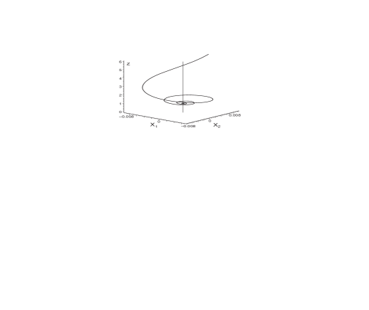
Inserting and in the polar Ansatz we obtain the final form of the self-similar solution for (at a given time the solution covers the and parts of the axis, while the interval is covered by the trivial solution ):
| (17) |
The constant phase is not interesting - it just corresponds to global rotations around the -axis. The minus sign present in formula (16) has been included in this phase. It is clear that the distance between the string and the -axis, equal to , quadratically grows from 0 at the points to when Much more interesting is the behaviour of the phase of at a fixed time . It describes the winding of the string around the -axis. At the phase is equal to . When decreases, the phase increases by with each step from to , where
(we have assumed here that . Thus, the string winds around the -axis infinitely many times as . Similar behaviour of the phase is found when , the only difference is that the string winds in the opposite direction.
Such unusual behaviour of the string might create a suspicion that it is unphysical for the following reason: that there is an infinite amount of energy accumulated in the finite region around the point (and, symmetrically, around ). It turns out that this is not the case. The total energy of the piece of the string between the points with the coordinates and , where , is given by the formula
Elementary calculation shows that
Furthermore, the length of that piece of the string is also finite:
The last formula is valid for and .
Let us notice that if we put , then and the solution has the simple form
This particular solution coincides with one of self-similar solutions of signum-Gordon equation considered in [3]. In this case the string lies in one plane containing the -axis. Solutions with are more general - the string winds around the -axis. In the case of Eq. (12) has the same form as in the signum-Gordon model [3]. Thus, the ‘centrifugal’ term in Eq. (12) is the only effect of presence of the second scalar field , as far as the self-similar solutions are concerned.
Solution (17) can be regarded as the solution of an initial value problem for the string being pinned to the -axis. The initial data are given at the time which corresponds to . Formula (17) implies that
| (18) |
Thus, at the initial moment all points of the string lie in one plane (the one with azimuthal angle ), and the initial velocities of the points of the string are perpendicular to their initial position vectors .
Let us end this Section with the observation that one can also obtain asymmetric solutions, i.e., such that for or for . The corresponding initial data are obtained by multiplying both formulas (18) by or . The point is that for corresponds to both and Therefore, Eq. (12) should actually be considered separately in the regions and , and there is no justification for a requirement of continuity of at !. For this reason we may take the trivial solution in the whole region and in the interval , or for all and for . These choices give the asymmetric solutions. On the other hand, notice that and correspond to . Therefore, the behaviour of at is correlated with the behaviour at because the function is continuous at . However, this is not such a severe condition as it might seem because formula (8) for the function contains the factor which vanishes for - it relates only the terms in the function in the regions and .
3 Real scalar field in 2+1 dimensions
Let us consider a membrane (in three dimensional space) which is attracted to a plane. The plane is parametrised by the Cartesian coordinates , and the elevation of the membrane at the moment over the point of the plane is denoted by . We consider the membrane without overhangs, hence is a single valued, real function of . The evolution equation has the form
| (19) |
where denotes the two-dimensional Laplacian. The corresponding field theoretic potential again has the form (1), that is The scaling transformations which are the symmetry of Eq. (19) have the form
where .
For simplicity, we consider only the axially symmetric configurations, hence does not depend on the azimuthal angle. In this case the evolution equation has the form
| (20) |
where The self-similar Ansatz
| (21) |
reduces Eq. (20 ) to ordinary differential equation
| (22) |
where ′ denotes the derivative The corresponding homogeneous equation
| (23) |
has the following linearly independent solutions 333 has been obtained by inserting a polynomial Ansatz in Eq. (22), and from by the standard method [8]:
| (24) |
| (25) |
From them we can construct partial solutions of Eq. (22)
| (26) |
where are constants. In general, these solutions are valid only in certain finite intervals of the axis, determined by the inequalities - for this reason we have called them the partial solutions. There also exists the trivial solution (remember that ), and the static solutions
| (27) |
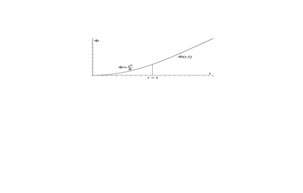
By glueing together these solutions one can produce various self-similar solutions of Eq. (22). We will present here just one class of such solutions, which describes how the membrane ‘freezes’ in the static position. These solutions involve the static solution and the partial solution which are glued together on the ‘light-cone’ , i.e., at the point , see Fig. 2. In accordance with Eq. (23), in this case it is sufficient to demand only continuity of . This condition has the form . Simple calculation shows that it is equivalent to the condition . Therefore, the corresponding solution of Eq. (20) has the following form
| (28) |
Here , and we have chosen that branch of for which Moreover,
| (29) |
This last condition ensures that on the whole half-line Thus, with time larger and larger part of the membrane becomes static. It follows from the explicit form (28) of the solution that at the initial time
| (30) |
If, for example, the initial slope of the parabola is smaller than 1/4 (), the initial velocity is positive, i.e., the parabola moves upwards towards the static shape. Notice, however, that this is done in a manner consistent with the causal dynamics implied by wave equation (20) - the freezing occurs at the front which travels with the finite velocity equal to +1.
One may expect that there are self-similar solutions of Eq. (19) which depend on the azimuthal angle in the plane. The angle is invariant under the rescaling . The Ansatz for self-similar solutions could be taken in the form . We have not investigated such solutions of Eq. (19).
4 -Gordon model in 1+1 dimensions
As pointed out in [1], the scaling symmetry (4) is shared by all (1+1)-dimensional models with V-shaped field potential
where are arbitrary real constants, denotes the step function 444 when and when ., and is a real scalar field. The corresponding wave equations have the form
| (31) |
We are interested in the models such that for the potential energy has minimum at . For this, we have to assume that In the particular case the potential is symmetric with respect to the reflection , and Eq. (31) becomes the signum-Gordon equation considered in [3]. Now we would like to investigate the self-similar solutions in the case when Eq. (31) has the form
| (32) |
For the obvious reason we will call this equation the -Gordon equation.
Physical context for considering equation of the form (32) is the depinning phenomenon. This equation can be regarded as describing the dynamics of a string in a plane which would be permanently pinned to the line were it not for a constant bias force, which exactly compensates the pinning force on one side of the line ( is just the deviation of the string from this line). Hence, the -Gordon equation describes the dynamics of the string exactly at the depinning transition.
The Anstaz for self-similar solutions has the form
where . Inserting it in Eq. (32) we obtain the following equation
where ′ denotes the derivative . This equation is to be satisfied in the weak sense, hence we may drop the factor which differs from 1 only at the single point . Therefore, obeys (again in the weak sense) the following equation
| (33) |
Equation (33) has the trivial solutions which correspond, respectively, to and to the static solution
| (34) |
Furthermore, there are the partial solutions
| (35) |
where are constants. As in the previous Sections, the partial solutions are valid only in certain intervals of the axis, determined by the inequalities .
Glueing together the partial solutions one can obtain whole variety of self-similar solutions of Eq. (32)
[9]. We present here certain interesting examples.
1. Freezing in the static configuration.
This solution is depicted in Fig. 3.
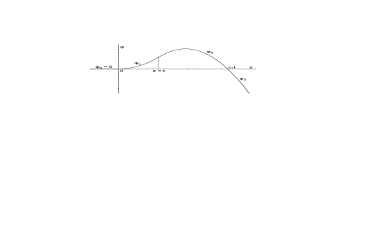
It has the following explicit form
| (36) |
where
and . The parameters are not independent – they have to obey the equation
| (37) |
which follows from the condition of continuity of the derivative at the point . It turns out that cubic equation (37) has three real solutions when . The relevant root obeys the inequality .
Initial configuration for solution (36) has the form
2. Depinning of the string from the z-axis.
The function has the shape presented in Fig. 4.
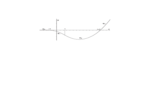
In this case
| (38) |
where , and
Solution (38) is valid provided that . This condition is satisfied if
| (39) |
5 Remarks
1. We have presented examples of self-similar solutions which describe rather interesting dynamical
processes like the freezing in the static configurations or the depinning. However, it is obvious that the
three models considered here have other self-similar solutions as well. In the case of -Gordon model one
can provide the complete list of such solutions [9] analogous to the one given in [3] for
signum-Gordon model. In the other two models such a complete list is probably out of our reach because of the
term in Eq. (12), or possible azimuthal angle dependence in the case of membrane model.
2. The kinetic part of evolution equation (3) contains d’Alembert operator , and this is standard for bosonic field. On the other hand, when we apply this equation in order to describe evolution of the string we automatically make certain assumptions about the kind of string we consider. The precise statement is that it is the string which has evolution equation of the form (3) when its world-sheet is parametrized by the coordinates . Of course, we would like to see a connection with Nambu-Goto string, which has evolution equation of the form
| (40) |
where , is the inverse to and
Let us take a slightly more general than Minkowskian space-time metric :
| (41) |
where is a constant (equal to 1 in the case of Minkowski space-time). Simple calculations show that Nambu-Goto equation (40) is reduced to the equation
when
| (42) |
Interesting possibility to satisfy the conditions (42) is to take a very small . This would correspond to the Nambu-Goto string (or a linear defect like a vortex) in an anisotropic medium which would effectively provide metric (41). The term in Eq. (3) represents the pinning force with which the line attracts the string.
Analogous remarks can be made about the membrane discussed in Section 3 and about the planar string of Section 4.
3. The V-shaped field potentials we consider should not be identified as potentials which
just contain the modulus of the pertinent field. Examples of such potentials can be found in [10, 11]. The
fundamental difference is that in our models the second derivative does not exist right at the minimum of
the potential, hence there is no preferred finite length (or mass) scale. Potentials considered in [10, 11]
have the shape. In these cases does not exist at a local maximum while at minima it exists –
that has much smaller impact on properties of the fields.
References
- [1] H. Arodź, P. Klimas and T. Tyranowski, Acta Phys. Pol. B36, 3861 (2005).
- [2] H. Arodź, P. Klimas and T. Tyranowski, Phys. Rev. E 73, 046609 (2006).
- [3] H. Arodź, P. Klimas and T. Tyranowski, arXiv: hep-th/0701148.
- [4] L. Debnath, Nonlinear Partial Differential Equations for Scientists and Engineers. Birkhäuser, Boston-Basel-Berlin, 2005. Chapter 8.
- [5] G. I. Barenblatt, Scaling, selfsimilarity, and intermediate asymptotics. Cambridge University Press, 1996.
- [6] R. D. Richtmyer, Principles of Advanced Mathematical Physics. Springer-Verlag, New York-Heidelberg-Berlin, 1978. Section 17.3.
- [7] L. C. Evans, Partial Differential Equations. American Math. Society, 1998.
- [8] G. A. Korn, T. M. Korn, Mathematical Handbook for Scientists and Engineers. McGraw-Hill Book Company, New York, 1961. Chapt. 9.3-8.
- [9] T. Tyranowski, Thesis for MSc Degree, Jagiellonian University, Cracow, 2007. Unpublished.
- [10] H. J. de Vega, Phys. Rev. D19 (1979) 3072.
- [11] S. Theodorakis, Phys. Rev. E56 (1997) 4809.