QCD Approach to $B\to D\pi$ Decays and CP Violation

Abstract

The branching ratios and CP violations of the $B\to D\pi$ decays, including both the color-allowed and the color-suppressed modes, are investigated in detail within QCD framework by considering all diagrams which lead to three effective currents of two quarks. An intrinsic mass scale as a dynamical gluon mass is introduced to treat the infrared divergence caused by the soft collinear approximation in the endpoint regions, and the Cutkosky rule is adopted to deal with a physical-region singularity of the on mass-shell quark propagators. When the dynamical gluon mass $\mu_{g}$ is regarded as a universal scale, it is extracted to be around $\mu_{g}=440$ MeV from one of the well-measured $B\to D\pi$ decay modes. The resulting predictions for all branching ratios are in agreement with the current experimental measurements. As these decays have no penguin contributions, there are no direct $CP$ asymmetries. Due to interference between the Cabibbo-suppressed and the Cabibbo-favored amplitudes, mixing-induced $CP$ violations are predicted in the $B\to D^{\pm}\pi^{\mp}$ decays to be consistent with the experimental data at 1-$\sigma$ level. More precise measurements will be helpful to extract weak angle $2\beta+\gamma$.

I Introduction

Nonleptonic $B$-meson decays are of crucial importance to deepen our insights into the flavor structure of the Standard Model (SM), the origin of CP violation, and the dynamics of hadronic decays, as well as to search for any signals of new physics beyond the SM. However, due to the non-perturbative strong interactions involved in these decays, the task is hampered by the computation of matrix elements between the initial and the final hadron states. In order to deal with these complicated matrix elements reliably, several novel methods based on the naive factorization approach (FA) Wirbel , such as the QCD factorization approach (QCDF) M , the perturbation QCD method (pQCD) lihn , and the soft-collinear effective theory (SCET) SCET , have been developed in the past few years. These methods have been used widely to analyze the hadronic $B$-meson decays, while they have very different understandings for the mechanism of those decays, especially for the case of heavy-light final states, such as the $B\to D\pi$ decays. Presently, all these methods can give good predictions for the color allowed $\overline{B}^{0}\to D^{+}\pi^{-}$ mode, but for the color suppressed $\overline{B}^{0}\to D^{0}\pi^{0}$ mode, the QCDF and the SCET methods could not work well, and the pQCD approach seems leading to a reasonable result in comparison with the experimental data. In this situation, it is interesting to study various approaches and find out a reliable approach.

As the mesons are regarded as quark and anti-quark bound states, the nonleptonic two body meson decays concern three quark-antiquark pairs. It is then natural to investigate the nonleptonic two body meson decays within the QCD framework by considering all Feynman diagrams which lead to three effective currents of two quarks. In our considerations, beyond these sophisticated pQCD, QCDF and SCET, we shall try to find out another simple reliable QCD approach to understand the nonleptonic two body decays. In this note, we are focusing on evaluating the $B\to D\pi$ decays.

The paper is organized as follows. In Sect. II, we first analyze the relevant Feynman diagrams and then outline the necessary ingredients for evaluating the branching ratios and $CP$ asymmetries of $B\to D\pi$ decays. In Sect. III, we list amplitudes of $B\to D\pi$ decays. The approaches for dealing with the physical-region singularities of gluon and quark propagators are given in Sect. IV. Finally, we discuss the branching ratios and the $CP$ asymmetries for those decay modes and give conclusions in Sects. V and VI, respectively. The detail calculations of amplitudes for these decay modes are given in the Appendix.

II Basic Considerations for Evaluating $B\to D\pi$ Decays

We start from the four-quark effective operators in the effective weak Hamiltonian, and then calculate all the Feynman diagrams which lead to effective six-quark interactions. The effective Hamiltonian for $\overline{B}\to D\pi$ decays can be expressed as

$${\cal H}_{eff}=\frac{G_{F}}{\sqrt{2}}V_{cb}V_{ud}^{*}[C_{1}(\mu)O_{1}(\mu)+C_{2}(\mu)O_{2}(\mu)]+{\rm h.c.},$$ (1)

where $C_{1}$ and $C_{2}$ are the Wilson coefficients which have been evaluated at next-to-leading order Buchalla , $O_{1}$ and $O_{2}$ are the tree operators arising from the $W$-boson exchanges with

$$\begin{array}[]{ll}O_{1}=(\bar{c}_{i}b_{i})_{V-A}(\bar{d}_{j}u_{j})_{V-A},&O_{2}=(\bar{c}_{i}b_{j})_{V-A}(\bar{d}_{j}u_{i})_{V-A},\end{array}$$ (2)

where $i$ and $j$ are the ${\rm SU(3)}$ color indices.

Based on the effective Hamiltonian in Eq. (1), we can then calculate the decay amplitudes for $\overline{B}^{0}\rightarrow D^{+}\pi^{-}$, $\overline{B}^{0}\rightarrow D^{0}\pi^{0}$, and $B^{-}\rightarrow D^{0}\pi^{-}$ decays, which are the color-allowed, the color-suppressed, and the color-allowed plus color-suppressed modes, respectively. All the six-quark Feynman diagrams that contribute to $\overline{B}^{0}\rightarrow D^{+}\pi^{-}$ and $B^{0}\rightarrow D^{0}\pi^{0}$ decays are shown in Figs. 1-3 via one gluon exchange. As for the process $B^{-}\rightarrow D^{0}\pi^{-}$, it doesn’t involve the annihilation diagrams and the related Feynman diagrams are the sum of Figs. 1 and 2. Based on the Isospin symmetry argument, the decay amplitude of this mode can be written as $A(B^{-}\rightarrow D^{0}\pi^{-})=A(\overline{B}^{0}\rightarrow D^{+}\pi^{-})-\sqrt{2}A(\overline{B}^{0}\rightarrow D^{0}\pi^{0})$. The explicit expressions for the amplitudes of these decay modes are given in detail in next section.

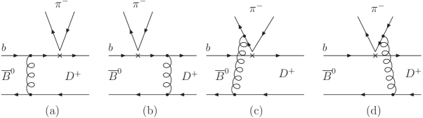
Figure 1: The factorizable ((a) and (b)) and nonfactorizable ((c) and (d)) diagrams contributing to the color-allowed $\overline{B}^{0}\rightarrow D^{+}\pi^{-}$ decay.

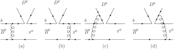
Figure 2: The factorizable ((a) and (b)) and nonfactorizable ((c) and (d)) diagrams contributing to the color-suppressed $\overline{B}^{0}\rightarrow D^{0}\pi^{0}$ decay.

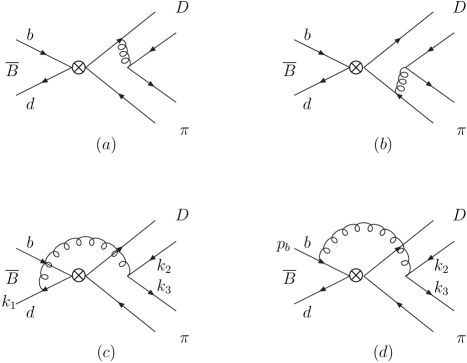
Figure 3: The annihilation diagrams for $\overline{B}^{0}\rightarrow D^{+}\pi^{-}$ and $\overline{B}^{0}\rightarrow D^{0}\pi^{0}$ decays.

The decay amplitudes of $B\to D\pi$ decay modes are quite different. For the color-allowed $\overline{B}^{0}\to D^{+}\pi^{-}$ mode, it is expected that the decay amplitude is dominated by the factorizable contribution $A_{fac}$ (from the diagrams (a) and (b) in Fig. 1), while the nonfactorizable contribution $A_{nonfac}$ (from the diagrams (c) and (d) in Fig. 1) has only a marginal impact. This is due to the fact that the former is proportional to the large coefficient $a_{1}=C_{1}+\frac{C_{2}}{N_{C}}\sim 1$, while the latter is proportional to the quite small coefficient $a_{2}=C_{2}+\frac{C_{1}}{N_{C}}\sim 0$. In addition, there is an addition color-suppressed factor $\frac{1}{N_{C}}$ in the nonfactorizable contribution $A_{nonfac}$. In contrast with the $\overline{B}^{0}\to D^{+}\pi^{-}$ mode, the nonfactorizable contribution $A_{nonfac}$ (from (c) and (d) diagrams in Fig. 2) in the $\overline{B}^{0}\to D^{0}\pi^{0}$ mode is proportional to the large coefficient $a_{1}=C_{1}+\frac{C_{2}}{N_{C}}\sim 1$, and even if with an additional color-suppressed factor $\frac{1}{N_{C}}$, its contribution is still larger than the factorizable one $A_{fac}$ (from (a) and (b) diagrams in Fig. 2) which is proportional to the quite small coefficient $a_{2}=C_{2}+\frac{C_{1}}{N_{C}}\sim 0$. Thus, it is predicted that the decay amplitude of this mode is dominated by the nonfactorizable contribution $A_{nonfac}$. As for the $B^{-}\to D^{0}\pi^{-}$ mode, since its amplitude can be written as the sum of the ones of the above two modes, it is not easy to see which one should dominate the total amplitude.

The branching ratio for $B\to D\pi$ decays can be expressed as follows in terms of the total decay amplitudes

$${\cal B}(B\to D\pi)=\frac{\tau_{B}\,p_{c}}{8\,\pi\,m_{B}^{2}}\,\left|{\cal A}(B\to D\pi)\right|^{2}\,$$ (3)

where $\tau_{B}$ is the lifetime of the $B$ meson, and $p_{c}$ is the magnitude of the momentum of the final-state particles $D$ and $\pi$ in the $B$-meson rest frame and given by

$$p_{c}=\frac{1}{2m_{B}}\sqrt{\left[m_{B}^{2}-(m_{D}+m_{\pi})^{2}\,\right]\,\left[m_{B}^{2}-(m_{D}-m_{\pi})^{2}\,\right]}\,.$$ (4)

As is well-known, the direct $CP$ violation in meson decays is non-zero only if there are two contributing amplitudes with non-zero relative weak and strong phases. The weak-phase difference usually arises from the interference between two different topological diagrams. For three $B\to D\pi$ decays, it is seen from the Feynman diagrams in Figs. 1-3 that there are no weak-phase differences, and hence no direct $CP$ violation in all these three modes, we shall then consider the mixing-induced $CP$ violation.

As the final states $D^{+}\pi^{-}$ can be produced both in the decays of $\overline{B}^{0}$ meson via the Cabibbo-favored ($b\to c$) and in the decays of $B^{0}$ meson via the doubly Cabibbo-suppressed ($b\to u$) tree amplitudes. The relative weak-phase difference between these two amplitudes is $-\gamma$ and, when combining with the $B^{0}-\overline{B}^{0}$ mixing phase, the total weak-phase difference is $-(2\beta+\gamma)$ to all orders in the small CKM parameter $\lambda$. Thus, the $B^{0}(\overline{B}^{0})\to D^{+}\pi^{-}$ decays can in principle be used to measure the weak phase $\gamma$, since the weak phase $\beta$ has been measured with high precision. The time-dependent $CP$ asymmetry of such decay modes is defined as:

$${\cal A}_{D^{+}\pi^{-}}(\Delta t) = \frac{\Gamma(\overline{B}^{0}\to D^{+}\pi^{-}(\Delta t))-\Gamma({B}^{0}\to D^{+}\pi^{-}(\Delta t))}{\Gamma(\overline{B}^{0}\to D^{+}\pi^{-}(\Delta t))+\Gamma({B}^{0}\to D^{+}\pi^{-}(\Delta t))}$$ (5)

$$\simeq -a_{\epsilon}+(a_{\epsilon}+a_{\epsilon^{\prime}}^{D^{+}\pi^{-}})\cos{(\Delta m_{B}\cdot t)}+a_{\epsilon+\epsilon^{\prime}}^{D^{+}\pi^{-}}\sin{(\Delta m_{B}\cdot t)}$$

$$\simeq S_{D^{+}\pi^{-}}\sin(\Delta mt)-C_{D^{+}\pi^{-}}\cos(\Delta mt),$$

where $\Delta m$ is the mass difference of the two eigenstates of $B_{d}$ mesons, and $S_{D^{+}\pi^{-}}$ and $C_{D^{+}\pi^{-}}$ are given as

$$S_{D^{+}\pi^{-}}=\frac{2Im(\lambda_{D^{+}\pi^{-}})}{1+|\lambda_{D^{+}\pi^{-}}|^{2}}=a_{\epsilon+\epsilon^{\prime}}^{D^{+}\pi^{-}},\hskip 28.45274ptC_{D^{+}\pi^{-}}=\frac{1-|\lambda_{D^{+}\pi^{-}}|^{2}}{1+|\lambda_{D^{+}\pi^{-}}|^{2}}=-(a_{\epsilon}+a_{\epsilon^{\prime}}^{D^{+}\pi^{-}}),$$ (6)

with

$$\lambda_{D^{+}\pi^{-}}=\frac{V^{*}_{tb}V_{td}\langle D^{+}\pi^{-}|H_{eff}|\overline{B}^{0}\rangle}{V_{tb}V^{*}_{td}\langle D^{+}\pi^{-}|H_{eff}|B^{0}\rangle}.$$ (7)

Where the rephase-invariant quantities $a_{\epsilon}$, $a_{\epsilon^{\prime}}$ and $a_{\epsilon+\epsilon^{\prime}}$ PW characterize the indirect, direct and mixing-induced CP violations respectively. As $a_{\epsilon}\ll 1$ for neutral $B$ system, we have $C_{D^{+}\pi^{-}}\simeq-a_{\epsilon^{\prime}}^{D^{+}\pi^{-}}$ which characterizes direct CP violation. Defining $g$ and $h$ as the amplitudes of $\overline{B}^{0}\rightarrow D^{+}\pi^{-}$ and $B^{0}\rightarrow D^{+}\pi^{-}$ decay modes, respectively, we can further express these two CP asymmetries as

$$C_{D^{+}\pi^{-}} = \frac{|h|^{2}-|g|^{2}}{|h|^{2}+|g|^{2}}=\frac{z^{2}-1}{z^{2}+1}$$ (8)

$$S_{D^{+}\pi^{-}} = \frac{-2|g||h|\sin(2\beta+\gamma+\delta)}{|h|^{2}+|g|^{2}}=\frac{-2z\sin(2\beta+\gamma+\delta)}{z^{2}+1},$$ (9)

where $z=|h/g|$, and $\delta={\rm arg}|h/g|$ represents the relative strong-phase difference between the two amplitudes $g$ and $h$.

Similarly, we can define another two $CP$-violating parameters $C_{D^{-}\pi^{+}}$ and $S_{D^{-}\pi^{+}}$ for the $B^{0}(\overline{B}^{0})\to D^{-}\pi^{+}$ decays

$$C_{D^{-}\pi^{+}}=\frac{1-\bar{z}^{2}}{1+\bar{z}^{2}},\hskip 28.45274ptS_{D^{-}\pi^{+}}=\frac{-2\bar{z}\sin(2\beta+\gamma-\delta)}{1+\bar{z}^{2}},$$ (10)

with the parameter $\bar{z}$ defined as $\bar{z}=|\bar{h}/\bar{g}|=z$. Here the amplitudes $\bar{h}$ and $\bar{g}$ are the charge conjugations of the amplitudes $h$ and $g$. Since the magnitude of the Cabibbo-suppressed decay amplitude $|h|$ is much smaller than that of the Cabibbo-favored decay amplitude $|g|$, the ratio $z$ should be quite small and is found to be about $0.02$ in our framework. Thus, to a very good approximation, $C_{D^{+}\pi^{-}}=-C_{D^{-}\pi^{+}}\simeq-1$, and the coefficients of the sine terms are given by

$$S_{D^{+}\pi^{-}}=-2z\sin(2\beta+\gamma+\delta)=a_{\epsilon+\epsilon^{\prime}}^{D^{+}\pi^{-}}\,,\hskip 28.45274ptS_{D^{-}\pi^{+}}=-2z\sin(2\beta+\gamma-\delta)=a_{\epsilon+\epsilon^{\prime}}^{D^{-}\pi^{+}}.$$ (11)

To compare with the current experimental data, one usually define the following two quantities, which are given by the combination of two $CP$-violating parameters $S_{D^{+}\pi^{-}}$ and $S_{D^{-}\pi^{+}}$,

$$a=(S_{D^{+}\pi^{-}}+S_{D^{-}\pi^{+}})/2\,,\hskip 28.45274ptc=(S_{D^{+}\pi^{-}}-S_{D^{-}\pi^{+}})/2,$$ (12)

which can provide constraints on the weak phase $2\beta+\gamma$ and the strong phase $\delta$.

III $B\to D\pi$ Decay Amplitudes

Using the methods given in the Appendix, we can get the $B\to D\pi$ decay amplitudes, which are composed of three parts: the factorizable contribution $A_{fac}$, the nonfactorizable contribution $A_{nonfac}$, and the annihilation contribution $A_{anni}$. The amplitude of $\overline{B}^{0}\to D^{+}\pi^{-}$ mode is found to be

$${\cal A}(\overline{B}^{0}\to D^{+}\pi^{-})=V_{cb}V^{*}_{ud}(A_{fac}+A_{nonfac}+A_{anni}),$$ (13)

with

$$A_{fac} = \frac{G_{F}}{\sqrt{2}}f_{B}f_{D}f_{\pi}\pi\alpha_{s}(\mu)(C_{1}+\frac{C_{2}}{N_{C}})\frac{C_{F}}{N_{C}}\int_{0}^{1}dx\int_{0}^{1}dy\,\phi_{B}(x)\phi_{D}(y)$$ (14)

$$\times \biggl{(}(-\bar{y}m_{B}^{2}+2m_{b}m_{B}-2\bar{y}m_{D}m_{B}+m_{b}m_{D})\frac{m_{B}^{2}}{D_{b}k^{2}}$$

$$+ (-m_{c}m_{B}-2\bar{x}m_{D}m_{B}-2m_{c}m_{D})\frac{m_{B}^{2}}{D_{c}k^{2}}\bigg{)},\,$$

where $D_{b}=m^{2}_{B}\bar{y}-m^{2}_{b}$, $D_{c}=-m^{2}_{B}x\bar{x}-m^{2}_{c}$ and $k^{2}=m^{2}_{B}x(x-y)$. $\phi^{\prime}s$ are the wave functions of mesons. For the $B$-meson wave function, we shall take the form given in h.y.cheng

$$\phi_{B}(\rho)=N_{B}\rho^{2}(1-\rho)^{2}\textrm{exp}\left[-\frac{1}{2}\left(\frac{\rho m_{B}}{\omega_{B}}\right)^{2}\right],$$ (15)

with $\omega_{B}=0.25~{}{\rm GeV}$, and $N_{B}$ being a normalization constant. The $D$ meson distribution amplitude is given by

$$\phi_{D}(y)=6y(1-y)[1+C_{D}(1-2y)],$$ (16)

with the shape parameter $C_{D}=0.8$. For the $\pi$ meson light cone wave functions, we use the asymptotic form as given in Refs. M.T ; Genon ; p.ball :

$$\phi(u)=\phi_{\sigma}(u)=6u\bar{u},\hskip 28.45274pt\phi_{\pi}(u)=1.$$ (17)

with $\bar{u}=1-u$.

$$A_{nonfac} = \frac{G_{F}}{\sqrt{2}}f_{B}f_{D}f_{\pi}\pi\alpha_{s}(\mu)(C_{2}+\frac{C_{1}}{N_{C}})\frac{C_{F}}{N_{C}^{2}}\int_{0}^{1}dx\int_{0}^{1}dy\int_{0}^{1}dz\,\phi_{B}(x)\phi_{D}(y)\phi(z)$$ (18)

$$\times \bigg{(}\big{(}(-x+z)m_{B}^{2}-(x-y)m_{D}m_{B}\big{)}\frac{m_{B}^{2}}{D_{d}k^{2}}$$

$$+ \big{(}(-2x+y+\bar{z})m_{B}^{2}-(x-y)m_{D}m_{B}\big{)}\frac{m_{B}^{2}}{D_{u}k^{2}}\biggl{)}\,,$$

where $D_{d}=m^{2}_{B}(x-y)(x-\bar{z})$ and $D_{u}=m^{2}_{B}(x-y)(x-z)$.

$$A_{anni} = \frac{G_{F}}{\sqrt{2}}f_{B}f_{D}f_{\pi}\pi\alpha_{s}(\mu)\frac{C_{F}}{N_{C}^{2}}\int_{0}^{1}dx\int_{0}^{1}dy\int_{0}^{1}dz\,\phi_{D}(y)\biggl{\{}$$ (19)

$$\times \biggl{[}(C_{2}+\frac{C_{1}}{N_{C}})\biggl{(}(\bar{z}m^{2}_{B}-2m_{c}m_{D})\phi(z)+\mu_{\pi}(m_{c}-2zm_{D}+4m_{D})\phi_{\pi}(z)$$

$$- \mu_{\pi}(m_{c}+2zm_{D})\frac{\phi_{\sigma}^{\prime}(z)}{6}\biggl{)}\frac{m_{B}^{2}}{D_{ca}k_{a}^{2}}+\biggl{(}-ym^{2}_{B}\phi(z)+2\mu_{\pi}m_{D}(y+1)\phi_{\pi}(z)\biggl{)}\frac{m_{B}^{2}}{D_{ua}k_{a}^{2}}\biggl{]}$$

$$+ (C_{1}+\frac{C_{2}}{N_{C}})\phi_{B}(x)\biggl{[}\biggl{(}\big{(}(\bar{x}-y)m_{B}+m_{b}\big{)}m^{2}_{B}\phi(z)+\mu_{\pi}m_{D}\big{(}(2x-\bar{y}-z)m_{B}$$

$$- 4m_{b}\big{)}\phi_{\pi}(z)+\mu_{\pi}m_{D}m_{B}(y-\bar{z})\frac{\phi_{\sigma}^{\prime}(z)}{6}\biggl{)}\frac{m_{B}}{D_{ba}k_{a}^{2}}$$

$$+ \biggl{(}(x-\bar{z})m^{2}_{B}\phi(z)-\mu_{\pi}m_{D}\big{(}(y-\bar{z})\frac{\phi_{\sigma}^{\prime}(z)}{6}+(2x-y-\bar{z})\phi_{\pi}(z)\big{)}\biggl{)}\frac{m^{2}_{B}}{D_{da}k_{a}^{2}}\biggl{]}\biggl{\}},$$

where $\phi_{\sigma}^{\prime}(z)=\frac{d\phi_{\sigma}(z)}{dz}$, $D_{ca}=m^{2}_{B}z-m^{2}_{c}$, $D_{ua}=m^{2}_{B}\bar{y}$, $D_{ba}=m^{2}_{B}(\bar{x}-y)(\bar{x}-z)-m^{2}_{b}$, $D_{da}=m^{2}_{B}(x-y)(x-z)$ and $k^{2}_{a}=m^{2}_{B}yz$. The annihilation contribution is found to be much smaller than the ones from the factorizable and the nonfactorizable diagrams. Numerically, it is negligible.

For the color-suppressed $\overline{B}^{0}\to D^{0}\pi^{0}$ decay, its amplitude can be written as

$${\cal A}(\overline{B}^{0}\to D^{0}\pi^{0})=-\frac{1}{\sqrt{2}}V_{cb}V^{*}_{ud}(A_{fac}+A_{nonfac}-A_{anni}),$$ (20)

with

$$A_{fac} = \frac{G_{F}}{\sqrt{2}}f_{B}f_{D}f_{\pi}\pi\alpha_{s}(\mu)(C_{2}+\frac{C_{1}}{N_{C}})\frac{C_{F}}{N_{C}}\int_{0}^{1}dx\int_{0}^{1}dz\,\phi_{B}(x)$$ (21)

$$\times \bigg{[}\biggl{(}(-\bar{z}m_{B}^{2}+2m_{b}m_{B})\phi(z)+\mu_{\pi}(2\bar{z}m_{B}-m_{b})\phi_{\pi}(z)$$

$$+ \mu_{\pi}\big{(}2(z+1)m_{B}+m_{b}\big{)}\frac{\phi_{\sigma}^{\prime}(z)}{6}\bigg{)}\frac{m_{B}^{2}}{D_{b}k^{2}}+2\mu_{\pi}\bar{x}\phi_{\pi}(z)\frac{m_{B}^{3}}{D_{d}k^{2}}\biggl{]},$$

here $D_{b}=m^{2}_{B}\bar{z}-m^{2}_{b}$, $D_{d}=m^{2}_{B}(x-\bar{y})(x-z)$ and $k^{2}=m^{2}_{B}x(x-z)$.

$$A_{nonfac} = \frac{G_{F}}{\sqrt{2}}f_{B}f_{D}f_{\pi}\pi\alpha_{s}(\mu)(C_{1}+\frac{C_{2}}{N_{C}})\frac{C_{F}}{N_{C}^{2}}\int_{0}^{1}dx\int_{0}^{1}dy\int_{0}^{1}dz\,\phi_{B}(x)\phi_{D}(y)$$ (22)

$$\times \bigg{[}\biggl{(}\big{(}(\bar{x}-y)m_{B}^{2}+m_{c}m_{D}\big{)}\phi(z)+\mu_{\pi}m_{B}(x-z)\biggl{(}\phi_{\pi}(z)-\frac{\phi_{\sigma}^{\prime}(z)}{6}\biggl{)}\biggl{)}\frac{m_{B}^{2}}{D_{c}k^{2}}$$

$$+ \bigg{(}(-2x+y+z)m_{B}\phi(z)-\mu_{\pi}(x-z)\biggl{(}\phi_{\pi}(z)-\frac{\phi_{\sigma}^{\prime}(z)}{6}\biggl{)}\bigg{)}\frac{m_{B}^{3}}{D_{u}k^{2}}\biggl{]}\,,$$

where $D_{c}=-m^{2}_{B}x\bar{x}-m^{2}_{c}$ and $D_{u}=m^{2}_{B}(x-y)(x-z)$. For the annihilation amplitude $A_{anni}$, it is the same as the one in Eq. (19) since the two modes $D^{0}\pi^{0}$ and $D^{+}\pi^{-}$ have the same annihilation topological diagrams.

For the doubly Cabibbo-suppressed decay mode $\overline{B}^{0}\to D^{-}\pi^{+}$, its decay amplitude can be written as

$${\cal A}(\overline{B}^{0}\to D^{-}\pi^{+})=V_{ub}V^{*}_{cd}(A_{fac}+A_{nonfac}+A_{anni}),$$ (23)

here, $A_{fac},A_{nonfac}$ and $A_{anni}$ can be obtained from the ones of decay mode $\bar{B}^{0}\to D^{0}\pi^{0}$ by simply exchanging the Wilson coefficients $C_{1}$ and $C_{2}$.

For the $B^{-}\to D^{0}\pi^{-}$ decay, its amplitude can be yielded by using the isospin relation $A(B^{-}\rightarrow D^{0}\pi^{-})=A(\overline{B}^{0}\rightarrow D^{+}\pi^{-})-\sqrt{2}A(\overline{B}^{0}\rightarrow D^{0}\pi^{0})$.

IV Treatments for Physical-region Singularities

To perform a numerical calculation of the decay amplitudes of $B\to D\pi$ decays, the light-cone projectors of mesons are found to be very useful, and the details of these quantities are presented in the Appendix. Where one encounters the endpoint divergences stemming from the convolution integrals of the meson distribution amplitudes with the hard kernels, which is caused by the collinear approximation. To regulate such an infrared divergence, we may introduce an intrinsic mass scale realized in the symmetry-preserving loop regularizationLR ; LRC . At the tree level, it is equivalent to adopt an effective dynamical gluon mass in the propagator. Practically, such a gluon mass scale has been used to regulate the infrared divergences in the soft endpoint region Cornwall ; Yang ; kk

$$\frac{1}{k^{2}}~{}\Rightarrow~{}\frac{1}{k^{2}-\mu_{g}^{2}(k^{2})+i\epsilon}\,,\hskip 28.45274pt\mu_{g}^{2}(k^{2})=\mu_{g}^{2}\biggl{[}\frac{\ln(\frac{k^{2}+4\mu_{g}^{2}}{\Lambda^{2}})}{\ln(\frac{4\mu_{g}^{2}}{\Lambda^{2}})}\biggl{]}^{-\frac{12}{11}},$$ (24)

The use of this effective gluon propagator is supported by the lattice Williams and the field theoretical studies Alkofer , which have shown that the gluon propagator is not divergent as fast as $\frac{1}{k^{2}}$. Taking the hadronic scale $\Lambda=\Lambda_{QCD}$, the dynamical gluon mass scale can be determined from one of the well measured decay mode. Numerically, we will see that taking $\Lambda_{\rm QCD}=300$ MeV, the dynamical gluon mass scale is around $\mu_{g}=(1.5\pm 0.2)\Lambda_{\rm QCD}$.

Another physical-region singularity arises from the on mass-shell quark propagators. It can be easily checked that each Feynman diagram contributing to a given matrix element is entirely real unless some denominators vanish with a physical-region singularity, so that the $i\epsilon$ prescription for treating the poles becomes relevant. In other words, a Feynman diagram will yield an imaginary part for the decay amplitudes only when the virtual particles in the diagram become on mass-shell, thus the diagram may be considered as a genuine physical process. The Cutkosky rules cutkosky give a compact expression for the discontinuity across the cut arising from a physical-region singularity. When applying the Cutkosky rules to deal with a physical-region singularity of quark propagators, the following formula holds

$$\frac{1}{(k_{1}-k_{2}-k_{3})^{2}+i\epsilon} = P\biggl{[}\frac{1}{(k_{1}-k_{2}-k_{3})^{2}}\biggl{]}-i\pi\delta[(k_{1}-k_{2}-k_{3})^{2}],$$ (25)

$$\frac{1}{(p_{b}-k_{2}-k_{3})^{2}-m_{b}^{2}+i\epsilon} = P\biggl{[}\frac{1}{(p_{b}-k_{2}-k_{3})^{2}-m_{b}^{2}}\biggl{]}-i\pi\delta[(p_{b}-k_{2}-k_{3})^{2}-m_{b}^{2}],$$ (26)

where $P$ denotes the principle-value prescription. The role of the $\delta$ function is to put the particles corresponding to the intermediate state on their positive energy mass-shell, so that in the physical region, the individual Feynman diagram satisfies the unitarity condition. Equations (25) and (26) will be applied to the quark propagators $D_{da}$ and $D_{ba}$ in Equation (19), respectively. It is then seen that the possible large imaginary parts arise from the virtual quarks across their mass shells as physical-region singularities.

V Numerical Results

It is seen that for theoretical predictions it depends on many input parameters, such as the Wilson coefficient functions, the CKM matrix elements, the hadronic parameters, and so on. To carry out a numerical calculation, we take the following input parameters yao

$$\begin{array}[]{llll}C_{1}=1.117(1.073),&C_{2}=-0.267(-0.179),&m_{B}=5.28~{}{\rm GeV},&m_{D}=1.87~{}{\rm GeV},\\ m_{\pi^{\pm}}=139.6~{}{\rm MeV},&m_{\pi^{0}}=135~{}{\rm MeV},&m_{b}=4.66~{}{\rm GeV},&m_{c}=1.47~{}{\rm GeV},\\ f_{B^{0}}=216\pm 19~{}{\rm MeV},&f_{D}=223\pm 17~{}{\rm MeV},&f_{\pi}=130.1~{}{\rm MeV},&\tau_{B^{0}}=1.536~{}{\rm ps},\\ \tau_{B^{-}}=1.638~{}{\rm ps},&V_{ud}=1-\lambda^{2}/2,&V_{ub}=A\lambda^{3}(\rho-i\eta),&V_{cd}=-\lambda,\\ V_{cb}=A\lambda^{2}.\end{array}$$ (27)

The Wolfenstein parameters of the CKM matrix elements are taken as Charles:2004jd : $\lambda=0.2272\pm 0.001,~{}A=0.806\pm 0.014,~{}\bar{\rho}=0.195^{+0.024}_{-0.067},~{}\bar{\eta}=0.326^{+0.032}_{-0.015}$, with $\bar{\rho}=\rho(1-\frac{\lambda^{2}}{2}),~{}\bar{\eta}=\eta(1-\frac{\lambda^{2}}{2})$. The coefficient of the twist-3 distribution amplitude of the pseudoscalar $\pi$ meson is chosen as $\mu_{\pi}=1.5\pm 0.2~{}{\rm GeV}$ M ; bn .

With the above values for the input parameters, we are able to calculate the contributions of different amplitudes for each decay mode. Our final results at $m_{b}/2$ scale are presented in Table 1.

Table 1: Numerical results at $m_{b}/2$ scale of the amplitudes for different diagrams in $B\to D\pi$ decays. Amplitudes $A_{fac},A_{nonfac}$, and $A_{anni}$ represent the factorizable ((a)and (b) diagrams in Figs. 1 or 2), the non-factorizable ((c) and (d) diagrams in Figs. 1 or 2), and the annihilation (diagrams in Fig. 3) contributions, respectively.

Decay modes	$A_{fac}$	$A_{nonfac}$	$A_{anni}$
$\overline{B}^{0}\to D^{+}\pi^{-}$	$-2.2655-0.0060i$	$0.2613-0.1862i$	$-0.0047+0.0053i$
$\overline{B}^{0}\to D^{-}\pi^{+}$	$1.7865-0.0556i$	$-0.0447+0.0970i$	$0.0008-0.0017i$
$\overline{B}^{0}\to D^{0}\pi^{0}$	$-0.0603+0.0011i$	$0.6991-0.0022i$	$0.0010+0.0009i$
$B^{-}\to D^{0}\pi^{-}$	$-2.3375-0.2310i$	$-0.4884-0.1484i$	$0$

As a consequence, we are led to the predictions for the quantities $z$ and $\delta$, as well as the branching ratios of all the $B\to D\pi$ decay modes. We present our “default results” of branching ratios and detailed error estimates corresponding to the different theoretical uncertainties caused from the above input parameters in Tables 2 and  3, respectively. The errors consist of three parts: the first one refers to the variation of the dynamical gluon mass scale; the second one arises from the uncertainty due to the CKM parameters $A,\lambda,\bar{\rho}$, and $\bar{\eta}$; the third one originates from the uncertainties due to the meson decay constants and the parameter $\mu_{\pi}$.

Table 2: The branching ratios of $B\rightarrow D\pi$ decays with the default input parameters. The theoretical results in the second and the third lines correspond to the predictions at the $m_{b}/2$ and $m_{b}$ scales, respectively. The results correspond to $\mu_{g}=440~{}{\rm MeV}$.

Decay modes	$Br(m_{b}/2)$	$Br(m_{b})$	Experiment	Ref. Keum:2003js
$\overline{B}^{0}\to D^{+}\pi^{-}(10^{-3})$	$2.67$	$2.20$	$2.68\pm 0.12\pm 0.24\pm 0.12$ vonToerne:2003gc	$2.74^{+0.39}_{-0.37}$
			$2.63\pm 0.05\pm 0.22$ Aubert:2006cd
$B^{-}\to D^{0}\pi^{-}(10^{-3})$	$4.87$	$4.73$	$4.97\pm 0.12\pm 0.29\pm 0.22$ vonToerne:2003gc	$5.43^{+0.48}_{-0.47}$
			$4.90\pm 0.07\pm 0.23$  Aubert:2006cd
$\overline{B}^{0}\to D^{0}\pi^{0}(10^{-4})$	$2.17$	$2.04$	$2.89\pm 0.29\pm 0.38$  Aubert:2002yf	$2.5\pm 0.1$
			$2.25\pm 0.14\pm 0.35$Blyth:2006at
$\overline{B}^{0}\to D^{-}\pi^{+}(10^{-7})$	$5.54$	$4.78$	$-$	$-$

Table 3: The branching ratios of $B\rightarrow D\pi$ decays. The theoretical errors shown from left to right correspond to the uncertainties referred to as “dynamical gluon mass scale(upper one corresponding to $\mu_{g}=420~{}{\rm MeV}$ and the below one $\mu_{g}=460~{}{\rm MeV}$)”, “CKM parameters”, and “decay constants and the parameter $\mu_{\pi}$” as specified in the text.

Decay modes	$Br(m_{b}/2)$	$Br(m_{b})$
$\overline{B}^{0}\to D^{+}\pi^{-}(10^{-3})$	$2.67^{\,+0.47\,+0.62\,+0.91}_{\,-0.36\,-0.57\,-0.85}$	$2.20^{\,+0.52\,+0.16\,+0.80}_{\,-0.51\,-0.42\,-0.62}$
$B^{-}\to D^{0}\pi^{-}(10^{-3})$	$4.87^{\,+0.52\,+0.84\,+1.74}_{\,-0.48\,-0.50\,-0.31}$	$4.73^{\,+0.63\,+0.34\,+1.29}_{\,-0.44\,-0.89\,-1.18}$
$\overline{B}^{0}\to D^{0}\pi^{0}(10^{-4})$	$2.17^{\,+0.53\,+0.46\,+1.14}_{\,-0.45\,-0.46\,-0.89}$	$2.04^{\,+0.56\,+0.19\,+0.95}_{\,-0.33\,-0.50\,-0.75}$
$\overline{B}^{0}\to D^{-}\pi^{+}(10^{-7})$	$5.54^{\,+0.68\,+1.02\,+1.52}_{\,-0.44\,-0.97\,-1.38}$	$4.78^{\,+0.62\,+0.81\,+1.76}_{\,-0.48\,-1.10\,-1.38}$

From the numerical results given in Tables 1- 3, we arrive at the following observations:

(i) For the color-allowed (also Cabibbo-favored) decay mode $\overline{B}^{0}\rightarrow D^{+}\pi^{-}$, the factorizable contribution $A_{fac}$ dominates the total decay amplitude, while the contributions from $A_{nonfac}$ and $A_{anni}$ are small. In particular, the contribution of $A_{anni}$ is so small that we can safely neglect it in this decay mode. With the considered uncertainties, it is seen that our result is in agreement with the experimental data vonToerne:2003gc ; Aubert:2006cd , and also consistent with the one given in Keum:2003js : ${\cal B}(\overline{B}^{0}\rightarrow D^{+}\pi^{-})=(2.74^{+0.39}_{-0.37})\times 10^{-3}$ within the allowed theoretical uncertainties. The decay amplitude of its $CP$-conjugate decay mode $B^{0}\rightarrow D^{-}\pi^{+}$ can be obtained from that of $\overline{B}^{0}\rightarrow D^{+}\pi^{-}$ by changing the CKM element $V_{cb}V^{*}_{ud}$ to $V^{*}_{cb}V_{ud}$. Since these CKM elements are purely real, the branching ratio of $B^{0}\rightarrow D^{-}\pi^{+}$ decay is the same as that of $\overline{B}^{0}\rightarrow D^{+}\pi^{-}$ decay.

(ii) For the doubly Cabibbo-suppressed decay mode $\overline{B}^{0}\rightarrow D^{-}\pi^{+}$, the contributions from $A_{nonfac}$ and $A_{anni}$ are also much smaller than the one from $A_{fac}$. As the contributions are all proportional to the small CKM elements $|V_{ub}V^{*}_{cd}|$ $\sim\lambda^{4}$, the branching ratio of this decay mode is found to be at the order of $10^{-7}$, and much smaller than that of the Cabibbo-favored decay mode. Since the imaginary part of the dominated amplitude $A_{fac}$ is much smaller than the real part, the branching ratio of the $CP$-conjugate decay mode $B^{0}\rightarrow D^{+}\pi^{-}$ is approximately equal to that of the $\overline{B}^{0}\rightarrow D^{-}\pi^{+}$ decay.

(iii) For the color-suppressed decay mode $\overline{B}^{0}\to D^{0}\pi^{0}$, the contribution from $A_{nonfac}$ dominates the total decay amplitude. The result at the $m_{b}$ scale is smaller than that at the $m_{b}/2$ scale, but both are in agreement with the prediction given in Keum:2003js : ${\cal B}(\overline{B}^{0}\rightarrow D^{0}\pi^{0})=(2.5\pm 0.1)\times 10^{-4}$. The present central value at the $m_{b}/2$ scale agree well with the experimental data reported in Blyth:2006at , but slightly smaller than the recent experimental data given in Aubert:2002yf . While when considering their respective uncertainties, our prediction is still consistent with the experimental data.

(iv) For the $B^{-}\to D^{0}\pi^{-}$ decay, the main contribution originates from the factorizable one $A_{fac}$. Although its decay amplitude can be written as the color-favored $\overline{B}^{0}\rightarrow D^{+}\pi^{-}$ minus the color suppressed $\overline{B}^{0}\rightarrow D^{0}\pi^{0}$ decays, the branching ratio of this decay mode is enhanced compared to that of the latter two. The central values of our prediction are well consistent with the experimental data given in Aubert:2006cd ; vonToerne:2003gc . On the other hand, when taking into account of the theoretical uncertainties, our prediction is also consistent with the one given by the pQCD method Keum:2003js : ${\cal B}(B^{-}\to D^{0}\pi^{-})=(5.43^{+0.48}_{-0.47})\times 10^{-3}$.

(v) Although the branching ratios at the $m_{b}$ scale are smaller than those at the $m_{b}/2$ scale in all these decay modes, we can see that the final results have only a marginal dependence on the renormalization scale. As for the theoretical uncertainties in these decay modes, the errors originating from the dynamical gluon mass scale $\mu_{g}$, the CKM matrix elements are comparable with each other when $\mu_{g}\in(420,460)~{}{\rm MeV}$. However, the uncertainty originating from the decay constants and $\mu_{\pi}$ are dominate in these decays, especially in $B^{-}\to D^{0}\pi^{-}$ and $\overline{B}^{0}\to D^{-}\pi^{+}$ modes.

It is also interesting to note that the $B\to D$ transition form factor, $F^{B\to D}=0.634$, extracted from (a) and (b) diagrams in Fig. 1 is in good agreement with the ones obtained from the other methods, such as: $F^{B\to D}(0)=0.648$ (pQCD method Kurimoto:2002sb ); $F^{B\to D}(0)=0.690$ (Bauer-Stech-Wirbel(BSW) model Wirbel ); $F^{B\to D}(0)=0.636$ (Neubert-Stech(NS) model Neubert:1997uc ).

We now turn to discuss the $CP$ asymmetries in $B\to D\pi$ decays. As has already been discussed above, there are no direct $CP$ violations in all these decay modes. In the following discussions, we focus mainly on the time-dependent $CP$ asymmetries of $B\to D^{\pm}\pi^{\mp}$ decays.

Using the relevant formulas presented in the previous sections, we can predict the $CP$ asymmetries in $B\to D^{\pm}\pi^{\mp}$ decays and constrain the CKM angle $2\beta+\gamma$ through the two observables $a$ and $c$. Firstly, we present the results of the quantities $z$ and $\delta$ in Table 4. Taking the current constraints for the weak angles $\beta$ and $\gamma$ in the SM, we present our predictions for the $CP$ asymmetries $S_{D^{+}\pi^{-}}$ and $S_{D^{-}\pi^{+}}$, as well as the two observables $a$ and $c$. Secondly, taking the weak angles $\beta$ and $\gamma$ as free parameters, we show the dependence of the parameters $S_{D^{+}\pi^{-}},S_{D^{-}\pi^{+}}$ and the observables $a$, $c$ on the angle $2\beta+\gamma$ in Figs. 4 and 5, respectively.

Table 4: The $CP$ asymmetries for $B\to D^{\pm}\pi^{\mp}$ decays. The results in the middle row denote our theoretical predictions for each quantity. The center values correspond to $\mu_{g}=1.5\Lambda_{\rm QCD}$, and the error bars originate from the dynamical gluon mass scale with the upper one corresponding to $\mu_{g}=1.3\Lambda_{\rm QCD}$ and the below one $\mu_{g}=1.7\Lambda_{\rm QCD}$. The results in last row are the experimental data.

results	$z$	$\delta$	$S_{D^{+}\pi^{-}}$	S${}_{D^{-}\pi^{+}}$	$a$	$c$
Theor	$0.017^{+0.03}_{-0.01}$	$1.07^{+0.14}_{-0.04}$	$-0.010^{+0.004}_{-0.001}$	$-0.023^{+0.001}_{-0.001}$	$-0.017^{+0.003}_{-0.001}$	$0.007^{+0.002}_{-0.001}$
Exp Barberio:2006bi	$-$	$-$	$-$	$-$	$-0.030\pm 0.017$	$-0.022\pm 0.021$

From Table 4 and Figs. 4 and 5, we come to the following observations.

• (i) For $B\to D^{\pm}\pi^{\mp}$ decay modes, although there are large strong phase difference between the Cabibbo-suppressed and the Cabibbo-favored decay amplitudes, the $CP$-violating parameters $S_{D^{+}\pi^{-}}$ and $S_{D^{-}\pi^{+}}$ are found to be small ($-0.01\sim-0.02$) due to the smallness of the ratio $z$ ( $\simeq 0.02$). In addition, due to our predictions for the two parameters $S_{D^{+}\pi^{-}}$ and $S_{D^{-}\pi^{+}}$ are comparable to each other for a given dynamical gluon mass scale, the value for the parameter $c$ is nearly zero.

• (ii) The $CP$-violating parameters $S_{D^{+}\pi^{-}}$ and $S_{D^{-}\pi^{+}}$ are not sensitive to the choice of the dynamical gluon mass scale, especially when the dynamical gluon mass scale is chosen above the central value $1.5\Lambda_{\rm QCD}$. However, both of them have a strong dependence on the weak angle $2\beta+\gamma$. The same conclusion is also applied to the two observables $a$ and $c$. Our predictions for the two observables are consistent with experimental data when considering the corresponding uncertainties. Unfortunately, it is found that with the angle $2\beta+\gamma$ varying within the range $(0,180^{\circ})$, almost all of the values for $a$ and $c$ are in the range of the experimental data, which indicates that although direct constraints on the angle $2\beta+\gamma$ could be obtained through these parameters, the present experimental accuracy is insufficient to improve the knowledge of the apex in the unitarity plane. It is expected that more precise measurements in future experiments allow us to extract the angle $2\beta+\gamma$.

Figure 4: The $CP$-violating parameters $S_{D^{+}\pi^{-}}$ and $S_{D^{-}\pi^{+}}$ for $B\to D^{\pm}\pi^{\mp}$ decays as functions of the weak phase $2\beta+\gamma$ (in degree). The dashed, solid, and dash-dotted lines correspond to $\mu_{g}=1.3,1.5$ and $1.7\Lambda_{\rm QCD}$, respectively.

Figure 5: The same as Fig. 4, but for $CP$ observables $a$ and $c$.

VI Conclusions

In summary, we have calculated the decay amplitudes, strong phases, branching ratios, and $CP$ asymmetries for the $B\to D\pi$ decays, including both the color-allowed and the color-suppressed modes. It has been shown that these decay modes are theoretically clean as there are no penguin contributions. As a consequence, direct $CP$ violations are absent. The contributions from the factorizable diagrams dominate all the decay amplitudes except for the $\overline{B}^{0}\to D^{0}\pi^{0}$ process. All our predictions for branching ratios are consistent with the existing measurements. For the $\overline{B}^{0}\to D^{-}\pi^{+}$ mode, our predictions will be faced with the future experiments as no data are available at present. Due to small interference effects between the Cabibbo-suppressed and the Cabibbo-favored amplitudes, the non-zero $CP$-violating parameters $S_{D^{+}\pi^{-}}$ and $S_{D^{-}\pi^{+}}$ have been predicted in the $B\to D^{\pm}\pi^{\mp}$ decay modes. It has been shown that the $CP$-violating parameters have a strong dependence on the weak phase $2\beta+\gamma$, but they are not sensitive to the dynamical gluon mass scale. With the angle $2\beta+\gamma$ varying within the range $(0,180^{\circ})$, almost all of the values for the CP-violating parameters $a$ and $c$ are within the range of the current experimental data. Thus no constraints on the weak phase $2\beta+\gamma$ could be obtained through those parameters based on the current experiment data, and more precise measurements are needed in future experiments.

In this paper, we have further shown that the divergence treatments used in our previous work kk are reliable. Namely, the endpoint divergence caused by the soft collinear approximation in gluon propagator could be simply avoided by adopting the Cornwall prescription for the gluon propagator with a dynamical mass scale. Note that when the intrinsic mass is appropriately introduced, it may not spoil the gauge symmetry as shown recently in the symmetry-preserving loop regularization LR . Meanwhile, for the physical-region singularity of the on-mass-shell quark propagators, it can well be treated by applying for the Cutkosky rules. The combination of these two treatments for the endpoint divergences of gluon propagator and the physical-region singularity of the quark propagators enables us to obtain reasonable results, which are consistent with the existing experimental data and also in agreement with the ones Keum:2003js obtained by using the pQCD approach. However, this is different from the treatment of the latter, where $k_{T}^{2}$ and Sudakov factors have been used to avoid the endpoint divergence.

It is noted that the resulting predictions for the branching ratios are in general scale dependence on the dynamical gluon mass which plays the role of the IR cut-off. This dependence should in principle be compensated from the possible scale in the wave functions which characterizes the nonperturbative effects. In our approach, the dynamical gluon mass may be regarded as a universal scale to be fixed from one of the decay modes. For instance, in our present considerations, if the decay mode $\bar{B}^{0}\to D^{+}\pi^{-}$ is taken to extract the dynamical gluon mass scale, we have $\mu_{g}\simeq 440$ MeV, and the resulting predictions for other decay modes can serve as a consistent check. Within the current experimental errors and theoretical uncertainties for some relevant parameters, it is seen that our treatment is reliable. In order to further check the validity of the gluon-mass regulator method adopted to deal with the endpoint divergence, it is useful to extend this method to more decay modes. Anyway, the treatments presented in this paper may enhance its predictive power for analyzing non-leptonic $B$-meson decays.

Appendix: Detail calculations of the $B\to D\pi$ decays amplitudes

To evaluate the hadronic matrix elements of $B\to D\pi$ decays, the meson light-cone distribution amplitudes play an important role. In the heavy quark limit, the light-cone projectors for $B$, $D$ and $\pi$ mesons in momentum space can be expressed, respectively, as M.T

$${\cal M}_{\alpha\beta}^{B} = -\frac{if_{B}}{4}\,[(m_{B}+\not\!P_{1}\,)\,\gamma_{5}\,\phi_{B}(\rho)]_{\alpha\beta},$$

$${\cal M}_{\alpha\beta}^{D} = \frac{if_{D}\,}{4}\,[(\not\!P_{2}\,+m_{D})\,\gamma_{5}\,\phi_{D}(y)]_{\alpha\beta},$$

$${\cal M}_{\delta\alpha}^{\pi} = \frac{if_{P}}{4}\,\biggl{\{}\not\!P_{3}\,\gamma_{5}\,\phi(u)-\mu_{P}\gamma_{5}\biggl{(}\phi_{p}(u)-i\sigma_{\mu\nu}n_{-}^{\mu}v^{\nu}\frac{\phi^{\prime}_{\sigma}(u)}{6}+i\sigma_{\mu\nu}P_{3}^{\mu}\frac{\phi_{\sigma}(u)}{6}\frac{\partial}{\partial k_{\bot\nu}}\biggl{)}\biggl{\}}_{\delta\alpha},$$ (28)

From the Feynman diagrams shown in Figs. 1-3, we can get the amplitudes for each decay mode using the relevant Feynman rules and the light-cone projectors listed in Eqs. (28).

For the tree diagrams of $\overline{B}^{0}\to D^{+}\pi^{-}$ mode shown in Fig. 1, the amplitudes of each diagrams can be written as

$$A^{\ref{tree}a} = if_{\pi}P_{3}^{\mu}\mathrm{Tr}\big{[}{\cal M}^{B}(-ig_{s}\gamma^{\alpha}T^{a}_{ij}){\cal M}^{D}\gamma_{\mu}(1-\gamma_{5})\frac{i}{\not\!k_{b}\,-m_{b}}(-ig_{s}\gamma^{\beta}T^{b}_{kl})\big{]}\frac{-ig_{\alpha\beta}\delta_{ab}}{k^{2}},$$

$$= -if_{\pi}g^{2}_{s}\frac{C_{F}}{N_{C}}\frac{1}{D_{b}k^{2}}\mathrm{Tr}\big{[}{\cal M}^{B}\gamma^{\alpha}{\cal M}^{D}\not\!P_{3}\,(1-\gamma_{5})(\not\!k_{b}\,+m_{b})\gamma_{\alpha}\big{]}$$

$$A^{\ref{tree}b} = if_{\pi}P_{3}^{\mu}\mathrm{Tr}\big{[}{\cal M}^{B}(-ig_{s}\gamma^{\alpha}T^{a}_{ij}){\cal M}^{D}(-ig_{s}\gamma^{\beta}T^{b}_{kl})\frac{i}{\not\!k_{c}\,-m_{c}}\gamma_{\mu}(1-\gamma_{5})\big{]}\frac{-ig_{\alpha\beta}\delta_{ab}}{k^{2}},$$

$$= -if_{\pi}g^{2}_{s}\frac{C_{F}}{N_{C}}\frac{1}{D_{c}k^{2}}\mathrm{Tr}\big{[}{\cal M}^{B}\gamma^{\alpha}{\cal M}^{D}\gamma_{\alpha}(\not\!k_{c}\,+m_{c})\not\!P_{3}\,(1-\gamma_{5})\big{]}$$

$$A^{\ref{tree}c} = \mathrm{Tr}\big{[}{\cal M}^{\pi}(-ig_{s}\gamma^{\alpha}T^{a}_{ij})\frac{i}{\not\!k_{d}\,}\gamma^{\mu}(1-\gamma_{5})\big{]}\mathrm{Tr}\big{[}{\cal M}^{B}(-ig_{s}\gamma^{\beta}T^{b}_{kl}){\cal M}^{D}\gamma_{\mu}(1-\gamma_{5})\big{]}\frac{-ig_{\alpha\beta}\delta_{ab}}{k^{2}},$$

$$= -g^{2}_{s}\frac{C_{F}}{N_{C}}\frac{1}{D_{d}k^{2}}\mathrm{Tr}\big{[}{\cal M}^{\pi}\gamma^{\alpha}\not\!k_{d}\,\gamma^{\mu}(1-\gamma_{5})\big{]}\mathrm{Tr}\big{[}{\cal M}^{B}\gamma_{\alpha}{\cal M}^{D}\gamma_{\mu}(1-\gamma_{5})\big{]}$$

$$A^{\ref{tree}d} = \mathrm{Tr}\big{[}{\cal M}^{\pi}\gamma^{\mu}(1-\gamma_{5})\frac{i}{\not\!k_{u}\,}(-ig_{s}\gamma^{\alpha}T^{a}_{ij})\big{]}\mathrm{Tr}\big{[}{\cal M}^{B}(-ig_{s}\gamma^{\beta}T^{b}_{kl}){\cal M}^{D}\gamma_{\mu}(1-\gamma_{5})\big{]}\frac{-ig_{\alpha\beta}\delta_{ab}}{k^{2}}$$ (29)

$$= -g^{2}_{s}\frac{C_{F}}{N_{C}}\frac{1}{D_{u}k^{2}}\mathrm{Tr}\big{[}{\cal M}^{\pi}\gamma^{\mu}(1-\gamma_{5})\not\!k_{u}\,\gamma^{\alpha}\big{]}\mathrm{Tr}\big{[}{\cal M}^{B}\gamma_{\alpha}{\cal M}^{D}\gamma_{\mu}(1-\gamma_{5})\big{]},$$

where $A^{\ref{tree}j}$ stands for the $j$th($j=a,b,c,d$) diagrams in Fig.1, $k_{m}$ and $k$ the momentum of $m$ quark propagator and gluon propagator, respectively. Furthermore, $D_{m}$ and $k^{2}$ represent for the $m$ quark propagator and gluon propagator, respectively.

In Fig. 1(a), the $\pi$ meson can be written as a decay constant since it originates from the vacuum. Inversing the fermi lines and writing down the $B$ meson projector ${\cal M}^{B}$, gluon vertex $-ig_{s}\gamma^{\alpha}T^{a}_{ij}$, $D$ meson projector ${\cal M}^{D}$, the four quark vertex $\gamma_{\mu}(1-\gamma_{5})$, b quark propagator $\frac{i}{\not\!k\,_{b}-m_{b}}$ and another gluon vertex $-ig_{s}\gamma^{\beta}T^{b}_{kl}$ in a trace one by one, and finally the gluon propagator $\frac{-ig_{\alpha\beta}\delta_{ab}}{k^{2}}$, we can get the amplitude $A^{\ref{tree}a}$. $A^{\ref{tree}b}$ can be calculated in a similar way. In Fig. 1(c), the $\pi$ meson can no longer be written as a decay constant any more since it exchanges a gluon with the spectator quark. Writing down the $\pi$ meson projector ${\cal M}^{\pi}$, gluon vertex $-ig_{s}\gamma^{\alpha}T^{b}_{ij}$, $d$ quark propagator $\frac{i}{\not\!k\,_{d}}$ and the four quark vertex $\gamma^{\mu}(1-\gamma_{5})$ in turn in one trace, and writing down the $B$ meson projector ${\cal M}^{B}$, gluon vertex $-ig_{s}\gamma^{\beta}T^{b}_{kl}$, $D$ meson projector ${\cal M}^{D}$ and the four quark vertex $\gamma_{\mu}(1-\gamma_{5})$ in the other trace one by one, and finally the gluon propagator $\frac{-ig_{\alpha\beta}\delta_{ab}}{k^{2}}$, we can get the amplitude $A^{\ref{tree}c}$. Similarly, we can get the amplitude $A^{\ref{tree}d}$. Summing up the former and the latter two quantities in Eq. (29), we can get the factorizable part $A_{fac}$ (Eq. (14)) and the nonfactorizable $A_{nonfac}$ (Eq. (18)), respectively.

As for the annihilation diagrams for $\overline{B}^{0}\to D^{+}\pi^{-}$ in Fig. 3, the amplitudes can be written as

$$A^{\ref{annihilation}a} = if_{B}P_{1}^{\mu}\mathrm{Tr}\big{[}{\cal M}^{D}(-ig_{s}\gamma^{\alpha}T^{a}_{ij})\frac{i}{\not\!k_{ca}\,-m_{c}}\gamma_{\mu}(1-\gamma_{5}){\cal M}^{\pi}(-ig_{s}\gamma^{\beta}T^{b}_{kl})\big{]}\frac{-ig_{\alpha\beta}\delta_{ab}}{k^{2}_{a}},$$

$$= -if_{B}g^{2}_{s}\frac{C_{F}}{N_{C}}\frac{1}{D_{ca}k^{2}_{a}}\mathrm{Tr}\big{[}{\cal M}^{D}\gamma^{\alpha}(\not\!k_{ca}\,+m_{c})\not\!P_{1}\,(1-\gamma_{5}){\cal M}^{\pi}\gamma_{\alpha}\big{]}$$

$$A^{\ref{annihilation}b} = if_{B}P_{1}^{\mu}\mathrm{Tr}\big{[}{\cal M}^{D}\gamma_{\mu}(1-\gamma_{5})\frac{i}{\not\!k_{ua}\,}(-ig_{s}\gamma^{\alpha}T^{a}_{ij}){\cal M}^{\pi}(-ig_{s}\gamma^{\beta}T^{b}_{kl})\big{]}\frac{-ig_{\alpha\beta}\delta_{ab}}{k^{2}_{a}},$$

$$= -if_{B}g^{2}_{s}\frac{C_{F}}{N_{C}}\frac{1}{D_{ua}k^{2}_{a}}\mathrm{Tr}\big{[}{\cal M}^{D}\not\!P_{1}\,(1-\gamma_{5})\not\!k_{ua}\,\gamma^{\alpha}{\cal M}^{\pi}\gamma_{\alpha}\big{]},$$

$$A^{\ref{annihilation}c} = \mathrm{Tr}\big{[}{\cal M}^{B}(-ig_{s}\gamma^{\alpha}T^{a}_{ij})\frac{i}{\not\!k_{da}\,}\gamma^{\mu}(1-\gamma_{5})\big{]}\mathrm{Tr}\big{[}{\cal M}^{D}\gamma_{\mu}(1-\gamma_{5}){\cal M}^{\pi}(-ig_{s}\gamma^{\beta}T^{b}_{kl})\big{]}\frac{-ig_{\alpha\beta}\delta_{ab}}{k^{2}_{a}}$$

$$= -g^{2}_{s}\frac{C_{F}}{N_{C}}\frac{1}{D_{da}k^{2}_{a}}\mathrm{Tr}\big{[}{\cal M}^{B}\gamma^{\alpha}\not\!k_{da}\,\gamma^{\mu}(1-\gamma_{5})\big{]}\mathrm{Tr}\big{[}{\cal M}^{D}\gamma_{\mu}(1-\gamma_{5}){\cal M}^{\pi}\gamma_{\alpha}\big{]},$$

$$A^{\ref{annihilation}d} = \mathrm{Tr}\big{[}{\cal M}^{B}\gamma^{\mu}(1-\gamma_{5})\frac{i}{\not\!k_{ba}-m_{b}\,}(-ig_{s}\gamma^{\alpha}T^{a}_{ij})\big{]}\mathrm{Tr}\big{[}{\cal M}^{D}\gamma_{\mu}(1-\gamma_{5}){\cal M}^{\pi}(-ig_{s}\gamma^{\beta}T^{b}_{kl})\big{]}\frac{-ig_{\alpha\beta}\delta_{ab}}{k^{2}_{a}},$$ (30)

$$= -g^{2}_{s}\frac{C_{F}}{N_{C}}\frac{1}{D_{ba}k^{2}_{a}}\mathrm{Tr}\big{[}{\cal M}^{B}\gamma^{\mu}(1-\gamma_{5})(\not\!k_{ba}\,+m_{b})\gamma^{\alpha}\big{]}\mathrm{Tr}\big{[}{\cal M}^{D}\gamma_{\mu}(1-\gamma_{5}){\cal M}^{\pi}\gamma_{\alpha}\big{]},$$

where $k_{ma}$ and $k_{a}$ stand for the momentum of $m$ quark propagator and gluon propagator, and $D_{ma}$ and $k^{2}$ represent for the $m$ quark propagator and gluon propagator in these annihilation diagrams, respectively. Summing up the four quantities in Eq. (30), we can get the annihilation contribution $A_{anni}$ (Eq. (19)) of this decay mode.

Similarly, as for the tree diagrams of $\overline{B}^{0}\to D^{0}\pi^{0}$ decay mode in Fig 2, its amplitudes can be written as follows

$$A^{\ref{tree2}a} = if_{D}P_{2}^{\mu}\mathrm{Tr}\big{[}{\cal M}^{B}(-ig_{s}\gamma^{\alpha}T^{a}_{ij}){\cal M}^{\pi}\gamma_{\mu}(1-\gamma_{5})\frac{i}{\not\!k_{b}\,-m_{b}}(-ig_{s}\gamma^{\beta}T^{b}_{kl})\big{]}\frac{-ig_{\alpha\beta}\delta_{ab}}{k^{2}},$$

$$= -if_{D}g^{2}_{s}\frac{C_{F}}{N_{C}}\frac{1}{D_{b}k^{2}}\mathrm{Tr}\big{[}{\cal M}^{B}\gamma^{\alpha}{\cal M}^{\pi}\not\!P_{2}\,(1-\gamma_{5})(\not\!k_{b}\,+m_{b})\gamma_{\alpha}\big{]},$$

$$A^{\ref{tree2}b} = if_{D}P_{2}^{\mu}\mathrm{Tr}\big{[}{\cal M}^{B}(-ig_{s}\gamma^{\alpha}T^{a}_{ij}){\cal M}^{\pi}(-ig_{s}\gamma^{\beta}T^{b}_{kl})\frac{i}{\not\!k_{d}\,}\gamma_{\mu}(1-\gamma_{5})\big{]}\frac{-ig_{\alpha\beta}\delta_{ab}}{k^{2}},$$

$$= -if_{D}g^{2}_{s}\frac{C_{F}}{N_{C}}\frac{1}{D_{d}k^{2}}\mathrm{Tr}\big{[}{\cal M}^{B}\gamma^{\alpha}{\cal M}^{\pi}\gamma_{\alpha}\not\!k_{d}\,\not\!P_{2}\,(1-\gamma_{5})\big{]},$$

$$A^{\ref{tree2}c} = \mathrm{Tr}\big{[}{\cal M}^{D}(-ig_{s}\gamma^{\alpha}T^{a}_{ij})\frac{i}{(\not\!k_{c}\,-m_{c})}\gamma^{\mu}(1-\gamma_{5})\big{]}\mathrm{Tr}\big{[}{\cal M}^{B}(-ig_{s}\gamma^{\beta}T^{b}_{kl}){\cal M}^{\pi}\gamma_{\mu}(1-\gamma_{5})\big{]}\frac{-ig_{\alpha\beta}\delta_{ab}}{k^{2}},$$

$$= -ig^{2}_{s}\frac{C_{F}}{N_{C}}\frac{1}{D_{c}k^{2}}\mathrm{Tr}\big{[}{\cal M}^{D}\gamma^{\alpha}(\not\!k_{c}\,+m_{c})\gamma^{\mu}(1-\gamma_{5})\big{]}\mathrm{Tr}\big{[}{\cal M}^{B}\gamma_{\alpha}{\cal M}^{\pi}\gamma_{\mu}(1-\gamma_{5})\big{]},$$

$$A^{\ref{tree2}d} = \mathrm{Tr}\big{[}{\cal M}^{D}\gamma^{\mu}(1-\gamma_{5})\frac{i}{\not\!k_{u}\,}(-ig_{s}\gamma^{\alpha}T^{a}_{ij})\big{]}\mathrm{Tr}\big{[}{\cal M}^{B}(-ig_{s}\gamma^{\beta}T^{b}_{kl}){\cal M}^{\pi}\gamma_{\mu}(1-\gamma_{5})\big{]}\frac{-ig_{\alpha\beta}\delta_{ab}}{k^{2}}$$ (31)

$$= -ig^{2}_{s}\frac{C_{F}}{N_{C}}\frac{1}{D_{u}k^{2}}\mathrm{Tr}\big{[}{\cal M}^{D}\gamma^{\mu}(1-\gamma_{5})\not\!k_{u}\,\gamma^{\alpha}\big{]}\mathrm{Tr}\big{[}{\cal M}^{B}\gamma_{\alpha}{\cal M}^{\pi}\gamma_{\mu}(1-\gamma_{5})\big{]}.$$

We can get the factorizable contribution $A_{fac}$ (Eq. (21)) and the nonfactorizable part $A_{nonfac}$ (Eq. (22)) by summing up the formerand the latter two quantities in Eq. (31).

As for the annihilation diagrams for $\overline{B}^{0}\to D^{0}\pi^{0}$ decay, its amplitude is the same as the one in Eq. (30) since the two modes $D^{0}\pi^{0}$ and $D^{+}\pi^{-}$ have the same annihilation topological diagrams, which are shown in Fig. 3.

For the doubly Cabibbo-suppressed decay mode $\overline{B}^{0}\to D^{-}\pi^{+}$, its decay amplitude can be similarly expressed as the ones in Eq. (31) due to the same topological structure in these two decay modes.

Finally, for the $B^{-}\to D^{0}\pi^{-}$ decay, since its Feynman diagrams are the sums of the color-allowed and the color-suppressed one, we can easily get its amplitudes using the above results.

References

• (1) M. Wirbel, B. Stech, and M. Bauer, Z. Phys. C 29, 637 (1985); M. Bauer, B. Stech, and M. Wirbel, Z. Phys. C 34, 103 (1987).
• (2) M. Beneke, G. Buchalla, M. Neubert, and C. T. Sachrajda, Phys. Rev. Lett. 83, 1914 (1999); Nucl. Phys. B591, 313 (2000); 606, 245 (2001).
• (3) H. n. Li and H. L. Yu, Phys. Rev. Lett. 74, 4388 (1995); Phys. Lett. B 353, 301 (1995); Y. Y. Keum, H. n. Li, and A. I. Sanda, Phys. Rev. D 63, 054008 (2001).
• (4) C. W. Bauer, S. Fleming, D. Pirjol and I. W. Stewart, Phys. Rev. D 63, 114020 (2001); C. W. Bauer, D. Pirjol and I. W. Stewart, Phys. Rev. Lett.  87, 201806 (2001); Phys. Rev. D 65, 054022 (2002); 65, 054022 (2002).
• (5) G. Buchalla, A. J. Buras, and M. E. Lautenbacher, Rev. Mod. Phys. 68, 1125 (1996).
• (6) W.F. Palmer and Y.L. Wu, Phys. Lett. B350 245 (1995).
• (7) H. Y. Cheng and K. C. Yang, Phys. Lett. B 511, 40 (2001); H. Y. Cheng and K. C. Yang, Phys. Rev. D 64, 074004 (2001).
• (8) M. Beneke and T. Feldmann, Nucl. Phys. B592, 3 (2001).
• (9) P. Ball and V. M. Braun, Nucl. Phys. B543, 201 (1999).
• (10) S. Descotes-Genon and C. T. Sachrajda, Nucl. Phys. B625, 239 (2002).
• (11) Y. L. Wu, Int. J. Mod. Phys. A18, 5363 (2003); Y. L. Wu, Mod. Phys. Lett. A19, 2191 (2004).
• (12) Y. L. Ma and Y. L. Wu, Phys. Lett. B647, 427 (2007); Y. L. Ma, Y. L.Wu, Int. J. Mod. Phys. A21, 6383 (2006).
• (13) J. M. Cornwall, Phys. Rev. D 26, 1453 (1982); J. M. Cornwall and J. Papavasiliou, Phys. Rev. D 40, 3474 (1989); 44, 1285 (1991).
• (14) S. B. Shalom, G. Eilam, and Y. D. Yang, Phys. Rev. D 67, 014007 (2003); Y. D. Yang, F. Su, G. R. Lu and H. J. Hao, Eur. Phys. J. C 44, 243 (2005).
• (15) F. Su, Y. L. Wu, Y. D. Yang and C. Zhuang, Eur. Phys. J. C 48, 401 (2006).
• (16) A. G. Williams et al., hep-ph/0107029 and references therein.
• (17) R. Alkofer and L. von Smekal, Phys. Rept. 353, 281 (2001); L. von Smekal, R. Alkofer, and A. Hauck, Phys. Rev. Lett. 79, 3591 (1997); D. Zwanziger, Phys. Rev. D 69, 016002 (2004); D. M. Howe and C. J. Maxwell, Phys. Lett. B 541, 129 (2002); Phys. Rev. D 70, 014002 (2004); A. C. Aguilar, A. A. Natale, and P. S. Rodrigues da Silva, Phys. Rev. Lett. 90, 152001 (2003); S. Furui and H. Nakajima, AIP Conf. Proc. 717, 685 (2004).
• (18) R.E. Cutkosky, J. Math. Phys. 1, 429 (1960).
• (19) W. M. Yao et al. [Particle Data Group], J. Phys. G 33 (2006) 1.
• (20) J. Charles et al. [CKMfitter Group], Eur. Phys. J. C 41, 1 (2005), updated results and plots available at: http://ckmfitter.in2p3.fr.
• (21) M. Beneke and M. Neubert, Nucl. Phys. B675, 333 (2003).
• (22) E. von Toerne [CLEO Collaboration], hep-ex/0301016.
• (23) B. Aubert [BABAR Collaboration], hep-ex/0610027.
• (24) Y. Y. Keum, T. Kurimoto, H. N. Li, C. D. Lu and A. I. Sanda, Phys. Rev. D 69, 094018 (2004).
• (25) B. Aubert et al. [BABAR Collaboration], hep-ex/0207092.
• (26) S. Blyth et al. [BELLE Collaboration], Phys. Rev. D 74, 092002 (2006).
• (27) T. Kurimoto, H. n. Li and A. I. Sanda, Phys. Rev. D 67, 054028 (2003).
• (28) M. Neubert and B. Stech, Adv. Ser. Direct. High Energy Phys. 15, 294 (1998).
• (29) E. Barberio et al. [Heavy Flavor Averaging Group (HFAG)], hep-ex/0603003, and online update at http://www.slac.stanford.edu/xorg/hfag.