Quantum Error Correction of Observables

Abstract

A formalism for quantum error correction based on operator algebras was introduced in beny07 via consideration of the Heisenberg picture for quantum dynamics. The resulting theory allows for the correction of hybrid quantum-classical information and does not require an encoded state to be entirely in one of the corresponding subspaces or subsystems. Here, we provide detailed proofs for the results of beny07 , derive a number of new results, and we elucidate key points with expanded discussions. We also present several examples and indicate how the theory can be extended to operator spaces and general positive operator-valued measures.

I Introduction

A new framework for quantum error correction was derived in beny07 through a Heisenberg picture reformulation of the Schrödinger approach to error correction, and an expansion of the notion of a quantum code to allow for codes determined by algebras generated by observables. As the approach generalizes standard quantum error correction (QEC) bennett96 ; knill97 ; shor95 ; steane96 ; gottesman96 and operator quantum error correction (OQEC) kribs05 ; kribs06 , we called the resulting theory “operator algebra quantum error correction” (OAQEC). An important feature of OAQEC is that it provides a formalism for the correction of hybrid quantum-classical information Kuper03 .

In this paper we provide proofs for the results stated in beny07 , and we establish a number of new results. In addition, we expose some of the finer points of the theory with discussions and several examples. We also outline how the theory can be extended to the case of operator spaces generated by observables and general positive operator-valued measures (POVMs).

We continue below by establishing notation and describing requisite preliminary notions. In the next section we present a detailed analysis of passive quantum error correction within the OAQEC framework. The subsequent section does the same for active quantum error correction. This is followed by an expanded discussion of the application to information flow from beny07 , and we conclude with a section on the operator space and POVM extension.

I.1 Preliminaries

Given a (finite-dimensional) Hilbert space $\mathcal{H}$, we let $\mathcal{L}(\mathcal{H})$ be the set of operators on $\mathcal{H}$ and let $\mathcal{L}_{1}(\mathcal{H})$ be the set of density operators on $\mathcal{H}$. We shall write $\rho$, $\sigma$, $\tau$ for density operators and $X$, $Y$, etc, for general operators. The identity operator will be written as ${\bf 1}$.

Noise models in quantum computing are described (in the Schrödinger picture) by completely positive trace-preserving (CPTP) maps $\mathcal{E}:\mathcal{L}(\mathcal{H})\rightarrow\mathcal{L}(\mathcal{H})$ NC00 . We shall use the term quantum channel to describe such maps. Every map $\mathcal{E}$ has an operator-sum representation $\mathcal{E}(\rho)=\sum_{a}E_{a}\rho E_{a}^{\dagger}$, where the operators $E_{a}$ are called the operation elements or noise operators for $\mathcal{E}$. The Hilbert-Schmidt dual map $\mathcal{E}^{\dagger}$ describes the corresponding evolution of observables in the Heisenberg picture. A set of operation elements for $\mathcal{E}^{\dagger}$ is given by $\{E_{a}^{\dagger}\}$. Trace preservation of $\mathcal{E}$ is equivalent to the requirement that $\mathcal{E}^{\dagger}$ is unital; that is, $\mathcal{E}^{\dagger}({\bf 1})={\bf 1}$.

A quantum system $A$ (or $B$) is a subsystem of $\mathcal{H}$ if $\mathcal{H}$ decomposes as $\mathcal{H}=(A\otimes B)\oplus\mathcal{K}$. Subspaces of $\mathcal{H}$ can clearly be identified as subsystems $A$ with one-dimensional ancilla ($\dim B=1$). An algebra $\mathcal{A}$ of operators on $\mathcal{H}$ that is closed under Hermitian conjugation is called a (finite-dimensional) C^∗-algebra, what we will simply refer to as an “algebra”. Algebras of observables play a key role in quantum mechanics vN55 and recently it has been shown that they can be used to encode hybrid quantum-classical information Kuper03 . Below we shall discuss further the physical motivation for considering algebras in the present setting. Mathematically, finite-dimensional C^∗-algebras have a tight structure theory that derives from their associated representation theory Dav96 . In particular, there is a decomposition of $\mathcal{H}$ into subsystems $\mathcal{H}=\oplus_{k}(A_{k}\otimes B_{k})\bigoplus\mathcal{K}$ such that with respect to this decomposition the algebra is given by

$$\mathcal{A}=\Big{[}\bigoplus_{k}\big{(}\mathcal{L}(A_{k})\otimes{\bf 1}_{B_{k}}\big{)}\Big{]}\,\,\bigoplus\,\,0_{\mathcal{K}}.$$ (1)

The algebras $\mathcal{L}(A_{k})\otimes{\bf 1}_{B_{k}}$ are referred to as the “simple” sectors of $\mathcal{A}$. We shall write $\mathcal{M}_{n}$ for the set of $n\times n$ complex matrices, and identify $\mathcal{M}_{n}$ with the matrix representations for elements of $\mathcal{L}(A)$ when $\dim A=n$ and an orthonormal basis for $A$ is fixed.

II Passive Error Correction Of Algebras

As the terminology suggests, the existence of a passive code for a given noise model implies that no active operation is required (beyond decoding) to recover quantum information encoded therein. Mathematically, it is quite rare for a generic channel to have passive codes. However, many of the naturally arising physical noise models include symmetries that do allow for such codes zanardi97 ; palma96 ; duan97 ; lidar98 ; knill00 ; zanardi01a ; kempe01 ; choi06 ; knill06 ; holbrook04 ; holbrook05 ; junge05 .

The following is the standard definition of a noiseless subsystem (and decoherence-free subspace when $\dim B=1$) in the Schrödinger picture. Suppose we have a decomposition of the Hilbert space $\mathcal{H}$ as $\mathcal{H}=(A\otimes B)\oplus\mathcal{K}$. As a notational convenience, we shall write $\rho\otimes\tau$ for the operator on $\mathcal{H}$ defined by $(\rho\otimes\tau)\oplus 0_{\mathcal{K}}$.

Definition 1.

We say that $A$ is a noiseless (or decoherence-free) subsystem for $\mathcal{E}$ if for all $\rho\in\mathcal{L}_{1}(A)$ and $\sigma\in\mathcal{L}_{1}(B)$ there exists $\tau\in\mathcal{L}_{1}(B)$ such that

$$\mathcal{E}(\rho\otimes\sigma)=\rho\otimes\tau.$$ (2)

The “decoherence-free” terminology is usually reserved for subspaces (when $\dim B=1$).

II.1 Decoherence-Free And Noiseless Subspaces And Subsystems In The
Heisenberg Picture

The following theorem gives an equivalent formulation of this definition in the Heisenberg picture, that is in terms of the evolution of observables, given by the dual channel $\mathcal{E}^{\dagger}$. We introduce the projector $P$ of $\mathcal{H}$ onto the subspace $A\otimes B$.

Theorem 2.

$A$ is a noiseless subsystem for $\mathcal{E}$ if and only if

$$P\,\mathcal{E}^{\dagger}(X\otimes{\bf 1})\,P=X\otimes{\bf 1}$$ (3)

for all operators $X\in\mathcal{L}(A)$

Proof. If $A$ is a noiseless subsystem for $\mathcal{E}$, then for all $X\in\mathcal{L}(A)$ we have

$$\text{Tr}(P{\mathcal{E}}^{\dagger}(X\otimes{\bf 1})P(\rho\otimes\sigma)) = \text{Tr}(\mathcal{E}^{\dagger}(X\otimes{\bf 1})(\rho\otimes\sigma))=\text{Tr}((X\otimes{\bf 1})\mathcal{E}(\rho\otimes\sigma))$$

$$= \text{Tr}(X\rho\otimes\tau)=\text{Tr}(X\rho)\text{Tr}(\tau)$$

$$= \text{Tr}(X\rho)=\text{Tr}((X\otimes{\bf 1})(\rho\otimes\sigma)).$$

This is true for all $\rho\in\mathcal{L}_{1}(A)$ and all $\sigma\in\mathcal{L}_{1}(B)$. By linearity it follows that $P\mathcal{E}^{\dagger}(X\otimes{\bf 1})P=X\otimes{\bf 1}$ for all $X\in\mathcal{L}(A)$.

Reciprocally, if we assume Eq. (3) to be true for all $X\in\mathcal{L}(A)$, then for all $\gamma\in\mathcal{L}_{1}(A\otimes B)$ we have

$$\text{Tr}(X\,\text{Tr}_{B}(P\mathcal{E}(\gamma)P)) = \text{Tr}((X\otimes{\bf 1})P\mathcal{E}(\gamma)P)=\text{Tr}(P\mathcal{E}^{\dagger}(X\otimes{\bf 1})P\gamma)$$

$$= \text{Tr}((X\otimes{\bf 1})\gamma)=\text{Tr}(X\,\text{Tr}_{B}(\gamma)),$$

where we have freely used the facts $P(X\otimes{\bf 1})P=X\otimes{\bf 1}$ and $P\gamma P=\gamma$. Since the above equation is true for all $X$, we have $\text{Tr}_{B}(P\mathcal{E}(\gamma)P)=\text{Tr}_{B}(\gamma)$ for all $\gamma\in\mathcal{L}_{1}(A\otimes B)$, which was shown in kribs06 to be equivalent to the definition of $A$ being a noiseless subsystem for $\mathcal{E}$. ∎

Note that Eq. (3) can be satisfied even if part of an observable $X\otimes{\bf 1}$ spills outside of the subspace $P\mathcal{H}$ under the action of $\mathcal{E}^{\dagger}$. The projectors $P$ in Eq. (3) show that the noiseless subsystem condition in the Heisenberg picture is only concerned with the “matrix corner” of $\mathcal{E}^{\dagger}(X\otimes{\bf 1})$ partitioned by $P$.

In some cases the equivalence of Eq. (2) and Eq. (3) can be seen from a different perspective. For a bistochastic or unital channel (those for which $\mathcal{E}({\bf 1})={\bf 1}$), the dual $\mathcal{E}^{\dagger}$ is also a channel. Then structural results for unital channels from kribs03 can be used to give an alternate realization of this equivalence, and passive codes may be computed directly from the commutant of the operation elements for $\mathcal{E}$. The simplest case would be for “self-dual” channels, those for which $\mathcal{E}^{\dagger}=\mathcal{E}$. Clearly, any $\mathcal{E}$ with Hermitian operation elements is self-dual. In particular, self-dual channels include all Pauli noise models, which are channels with operation elements belonging to the Pauli group, the group generated by tensor products of unitary Pauli operators $X$, $Y,$ $Z$.

As a further illustrative (non-unital) example, consider the single-qubit spontaneous emission channel NC00 given by $\mathcal{E}(\sigma)=\text{Tr}(\sigma)\,|0\rangle\langle 0|$. Here $P=|0\rangle\langle 0|$. This channel is implemented by operation elements $E_{0}=P$ and $E_{1}=|0\rangle\langle 1|$. Hence the dual channel is given by $\mathcal{E}^{\dagger}(\sigma)=P\sigma P+E_{1}^{\dagger}\sigma E_{1}$. The subspace $A$ spanned by the ground state $|0\rangle$ is a decoherence-free subspace for $\mathcal{E}$ (though it cannot be used to encode quantum information since $\dim A=1$). In this case, Eq. (3) is equivalent to the statement $P\mathcal{E}^{\dagger}(P)P=P$, which may be readily verified.

One can consider more general spontaneous emission channels with non-trivial decoherence-free subspaces. For instance, consider a qutrit noise model that describes spontaneous emission from the second excited state to the ground state. The corresponding channel is defined by $\mathcal{E}(\sigma)=P\sigma P+E\sigma E^{\dagger}$, where $P=|0\rangle\langle 0|+|1\rangle\langle 1|$ and $E=|0\rangle\langle 2|$. The subspace $P\mathbb{C}^{3}={\rm span}\,\{|0\rangle,|1\rangle\}$ is a single-qubit decoherence-free subspace for $\mathcal{E}$ since $\mathcal{E}(\sigma)=\sigma$ for all $\sigma=P\sigma P$. It is also easy to see in this case that Eq. (3) is satisfied since $P\mathcal{E}^{\dagger}(X)P=X$ for all $X\in\mathcal{L}(P\mathbb{C}^{3})$. Notice also in this example that $\mathcal{E}^{\dagger}$ can induce “spillage” from $P$ to $P^{\perp}$. Indeed, this can be seen immediately from the operator-sum representation for $\mathcal{E}^{\dagger}$; specifically, for all $X\in\mathcal{L}(P\mathbb{C}^{3})$ we have

$$\mathcal{E}^{\dagger}(X)=PXP+E^{\dagger}XE=X+\alpha\,|2\rangle\langle 2|,$$ (4)

where $\alpha=\langle 0|X|0\rangle$.

II.2 Conserved Algebras Of Observables

A POVM determined by a set of operators $X=\{X_{a}\}$ evolves via the unital CP-map $\mathcal{E}^{\dagger}$ in the Heisenberg picture. If for all $a$ we have $X_{a}=\mathcal{E}^{\dagger}(X_{a})$, then all the statistical information about $X=\{X_{a}\}$ has been conserved. Indeed, for any initial state $\rho$, we have $\text{Tr}(\rho X_{a})=\text{Tr}(\rho\mathcal{E}^{\dagger}(X_{a}))=\text{Tr}(\mathcal{E}(\rho)X_{a})$. Moreover, if we have control on the initial states, an expected feature in quantum computing, we can ask which elements are conserved if the state starts in a certain subspace $P\mathcal{H}$; that is, which elements satisfy $P\mathcal{E}^{\dagger}(X_{a})P=PX_{a}P$, or equivalently $\text{Tr}(X_{a}\,\mathcal{E}(P\rho P))=\text{Tr}(X_{a}\,P\rho P)$ for all $\rho\in\mathcal{L}_{1}(\mathcal{H})$. This, together with the Heisenberg characterization of Eq. (3), motivates the following definition.

Definition 3.

We shall say that a set $\mathcal{S}$ of operators on $\mathcal{H}$ is conserved by $\mathcal{E}$ for states in $P\mathcal{H}$ if every element of $\mathcal{S}$ is conserved; that is, if

$$P\,\mathcal{E}^{\dagger}(X)\,P=PXP\quad\forall X\in\mathcal{S}.$$ (5)

The focus of the present work is error correction for algebras generated by observables. Let us consider in more detail the physical motivation for considering algebras. In the Heisenberg picture a set of operators $\{X_{a}\}$ evolves according to the unital CP-map $\mathcal{E}^{\dagger}$ with elements $E_{a}^{\dagger}$ instead of $E_{a}$. If for all values of the label $a$ we have $X_{a}=\mathcal{E}^{\dagger}(X_{a})$ then all the statistical information about $X$ has been conserved by $\mathcal{E}$ as noted above. In such a scenario we say that $X_{a}$ is conserved by $\mathcal{E}$. In particular, if $X$ defines a standard projective measurement, $X=\sum_{a}p_{a}X_{a}$ with $X_{a}^{2}=X_{a}$ for all $a$, then the projectors $X_{a}$ linearly span the algebra they generate. Hence, in this case $\mathcal{E}$ conserves an entire commutative algebra. Therefore, focussing on the conservation (and more generally correction defined later) of sets of operators that have the structure of an algebra, apart from allowing a complete characterization, is also sufficient for the study of all the correctable projective observables.

Further observe that Eq. (5) applied to a set of observables that generate an (arbitrary) algebra gives a generalization of noiseless subsystems. Indeed, by Theorem 2 any subalgebra $\mathcal{A}$ of $\mathcal{L}(P\mathcal{H})$ for which all elements $X\in\mathcal{A}$ satisfy Eq. (5) is a direct sum of simple algebras, each of which encodes a noiseless subsystem (when $\dim A_{k}>1$ as in Eq. (1)). It is also important to note that given an algebra $\mathcal{A}$ conserved for states in $P\mathcal{H}$ (or more generally correctable as we shall see) quantum information cannot in general be encoded into the entire subspace $P\mathcal{H}$ for safe recovery, but rather into subsystems of $P\mathcal{H}$ determined by the splitting induced from the algebra structure of $\mathcal{A}$. These points will be further expanded upon in the discussion of Section III.2.

We now establish concrete testable conditions for passive error correction. Namely, these conditions are stated strictly in terms of the operation elements for a channel. This result was stated without proof in beny07 . The special case of simple algebras in the Schrödinger picture was obtained in kribs05 ; kribs06 . Techniques of choi06 are used in the analysis. We first present a simple lemma that will be used below.

Lemma 4.

Let $\mathcal{F}$ be a CP map with elements $F_{a}$. If $A\geq 0$ is such that $\mathcal{F}(A)=0$ then it follows that $AF_{a}=0$ for every element $F_{a}$.

Proof. If $\sum_{a}F_{a}^{\dagger}AF_{a}=0$ then for any state $|\psi\rangle$, $\sum_{a}\langle\psi|F_{a}^{\dagger}AF_{a}|\psi\rangle=0.$ Since each operator $F_{a}^{\dagger}AF_{a}$ is positive, this is a sum of nonnegative terms. Therefore each individual term must equal zero; $\langle\psi|F_{a}^{\dagger}AF_{a}|\psi\rangle=0$ for all $a$. This means that the vector $\sqrt{A}F_{a}|\psi\rangle$ is of norm zero, and therefore is the zero vector. This being true for all states $|\psi\rangle$, we must have that $\sqrt{A}F_{a}=0$, from which it follows that $AF_{a}=0$. ∎

Theorem 5.

Let $\mathcal{A}$ be a subalgebra of $\mathcal{L}(P\mathcal{H})$. The following statements are equivalent:

1. $\mathcal{A}$ is conserved by $\mathcal{E}$ for states in $P\mathcal{H}$.

2. $[E_{a}P,X]=0$ for all $X\in\mathcal{A}$ and all $a$.

Proof. If $[E_{a}P,X]=[E_{a}P,PXP]=0$ for all $a$, then

$$P\mathcal{E}^{\dagger}(X)P=\sum_{a}PE_{a}^{\dagger}XE_{a}P = \sum_{a}PE_{a}^{\dagger}PXPE_{a}P$$

$$= \sum_{a}PE_{a}^{\dagger}E_{a}PXP=P{\mathcal{E}}^{\dagger}({\bf 1})PXP=PXP=X.$$

Reciprocally, we assume that each $X\in\mathcal{A}$ satisfies $P\mathcal{E}^{\dagger}(X)P=PXP=X$. Consider a projector $Q\in\mathcal{A}$. We have $P\mathcal{E}^{\dagger}(Q)P=Q$ and hence $P\mathcal{E}^{\dagger}(Q^{\perp})P=PQ^{\perp}$. Therefore

$$Q^{\perp}P\mathcal{E}^{\dagger}(Q)PQ^{\perp}=Q^{\perp}\,Q\,Q^{\perp}=0,$$

and similarly $QP\mathcal{E}^{\dagger}(Q^{\perp})PQ=0$. By Lemma 4, this implies respectively $QE_{a}PQ^{\perp}=0$ and $Q^{\perp}E_{a}PQ=0$ for all $a$. Together these conditions imply

$$QE_{a}P=QE_{a}PQ=E_{a}PQ,$$

and thus $[E_{a}P,Q]=0$ for all $a$. Finally, note that since $\mathcal{A}$ is an algebra, then a generic element $Y\in\mathcal{A}$ can be written as a linear combination of projectors in $\mathcal{A}$. Therefore we also have $[E_{a}P,Y]=0$ for all $Y\in\mathcal{A}$, and this completes the proof. ∎

This theorem allows us to identify the largest conserved subalgebra of $\mathcal{L}(P\mathcal{H})$ conserved on the subspace $P\mathcal{H}$. Namely, a direct consequence of Theorem 5 is that the (necessarily $\dagger$-closed) commutant inside $\mathcal{L}(P\mathcal{H})$ of the operators $\{E_{a}P,PE_{a}^{\dagger}\}$ is the largest such algebra.

Corollary 6.

The algebra $\mathcal{A}=\{X\in\mathcal{L}(P\mathcal{H}):\forall a\,\,[X,E_{a}P]=[X^{\dagger},E_{a}P]=0\}$ is conserved on states in $P\mathcal{H}$ and contains all subalgebras of $\mathcal{L}(P\mathcal{H})$ conserved on states $P\mathcal{H}$.

Note that $P$ itself may not belong to this algebra, unless it satisfies $E_{a}P=PE_{a}P$. This special case was the case considered in choi06 . With other motivations in mind, the special case $P={\bf 1}$ was also derived in lindblad99 where it was shown that the full commutant of $\{E_{a},E_{a}^{\dagger}\}$ is the largest algebra inside the fixed point set of a unital CP map. (This in turn may be regarded as a weaker form of the fixed point theorem for unital channels kribs03 .)

Likely the most prevalent class of decoherence-free subspaces are the stabilizer subspaces for abelian Pauli groups, which give the starting point for the stabilizer formalism gottesman96 . On the $n$-qubit Hilbert space, let $s<n$ and consider the group $S$ generated by the Pauli phase flip operators $Z_{1},\ldots,Z_{s}$, where we have written $Z_{1}=Z\otimes{\bf 1}\otimes\ldots\otimes{\bf 1}$, etc. The joint eigenvalue-1 space for $S$ is a $2^{n-s}$-dimensional decoherence-free subspace for $\{Z_{j}:1\leq j\leq s\}$, called the “stabilizer subspace” for $S$. In the stabilizer formalism, any of the $2^{s}$ (necessarily $2^{n-s}$-dimensional) mutually orthogonal joint eigenspaces for elements of $S$ could be used individually to build codes, but the eigenvalue-1 space is used as a convenience. Each of these eigenspaces supports a full matrix algebra $\mathcal{M}_{k}$, where $k=2^{n-s}$. In the present setting these decoherence-free subspaces may be considered together, as they are defined by the structure of the commutant $S^{\prime}\cong\mathcal{M}_{k}^{(2^{s})}$. In particular, this entire algebra is conserved by any channel defined with operation elements given by linear combinations of elements taken from $S$.

Allowing other Pauli operators into the error group can result in non-conserved scenarios. For instance, consider the case $n=3$ and $s=2$. The algebra $S^{\prime}\cong\mathcal{M}_{2}^{(4)}$ is conserved by channels determined by elements of $S$ as above. However, it is not conserved by channels determined by elements of $G=\{Z_{1},Z_{2},X_{1}X_{2}\}$, even though the individual eigenvalue-1 stabilizer space is still a correctable code for $G$. This follows from Theorem 5 since $G$ properly contains $S$, and hence $G^{\prime}$ is properly contained in $S^{\prime}$. (In this case $P={\bf 1}$, and the largest conserved algebra is the full commutant $G^{\prime}$ of the error group.) Interestingly, there are still algebras conserved by channels determined by elements of $G$, since its commutant has the structure $G^{\prime}={\rm Alg}\{G\}^{\prime}\cong(I_{2}\otimes\mathcal{M}_{2})\oplus(I_{2}\otimes\mathcal{M}_{2})$.

Let us reconsider the special case in which the projector $P$ itself is one of the correctable observables. Most importantly, this guarantees that after evolution all states are back into the code $P\mathcal{H}$. Indeed, the probability that a state $\rho$ initially in the code is still in the code after evolution is then given by

$$p=\text{Tr}(\mathcal{\mathcal{E}}(\rho)P)=\text{Tr}(\rho P\mathcal{E}^{\dagger}(P)P)=\text{Tr}(\rho P)=1.$$ (6)

We note that this also guarantees a repetition of the noise map will be conserved.

A refinement of the proof of Theorem 5 yields the following result when the projector $P$ is conserved and belongs to the algebra of observables in question.

Theorem 7.

Let $\mathcal{A}$ be an algebra containing the projector $P$. The following statements are equivalent:

1. $\mathcal{A}$ is conserved by $\mathcal{E}$ for states in $P\mathcal{H}$.

2. $[E_{a}P,X]=0$ for all $X\in P{\mathcal{A}}P$ and all $a$.

Proof. If $[E_{a}P,X]=[E_{a}P,PXP]=0$ for all $a$, then $P\mathcal{E}^{\dagger}(X)P=PXP$ follows as above. On the other hand, if each $X\in\mathcal{A}$ satisfies $P\mathcal{E}^{\dagger}(X)P=PXP$, then note that for $X=P$ this yields $P\mathcal{E}^{\dagger}(P)P=P$ which implies $P\mathcal{E}^{\dagger}(P^{\perp})P=0$. Therefore, by Lemma 4, $P^{\perp}E_{a}P=0$, that is, $E_{a}P=PE_{a}P$ for all $a$. Hence for all $X\in\mathcal{A}$ we also have $P\mathcal{E}^{\dagger}(PXP)P=PXP.$ But the set $P\mathcal{A}P$ is itself an algebra, since $P$ belongs to $\mathcal{A}$, and hence is spanned by its projectors. The rest of the proof proceeds as above. ∎

III Active Error Correction Of Algebras

More generally, active intervention into a quantum system may be required for error correction. In particular, we should be able to protect a set of operators $\{X_{a}\}$ (which could define a POVM for instance) by acting with a channel $\mathcal{R}$ such that each $X_{a}$ is mapped by $\mathcal{R}^{\dagger}$ to one of the operators $Y_{a}=\mathcal{E}^{\dagger}(X_{a})$. That is, $\mathcal{R}^{\dagger}(X_{a})=Y_{a}$, and thus $(\mathcal{R}\circ\mathcal{E})^{\dagger}(X_{a})=X_{a}$. This, together with the previous discussions, motivates the following definition.

Definition 8.

We say that a set $\mathcal{S}$ of operators on $\mathcal{H}$ is correctable for $\mathcal{E}$ on states in the subspace $P\mathcal{H}$ if there exists a channel $\mathcal{R}$ such that $\mathcal{S}$ is conserved by $\mathcal{R}\circ\mathcal{E}$ on states in $P\mathcal{H}$; in other words,

$$P(\mathcal{R}\circ\mathcal{E})^{\dagger}(X)P=PXP\quad\forall X\in\mathcal{S}.$$ (7)

This equation is the same as the one we used to defined passive error correction, except that we now allow for an arbitrary “correction operation” $\mathcal{R}$ after the channel has acted. In particular, as in other settings, the passive case may be regarded as the special case of active error correction for which the correction operation is trivial, $\mathcal{R}={\rm id}$.

This notion of correctability is more general than the one addressed by the framework of OQEC, and extends the one introduced in beny07 from algebras to arbitrary sets of observables. Here we shall continue to focus on algebras, and in Section V we consider an extension of the notion to general operator spaces. Whereas OQEC focusses on simple algebras, $\mathcal{L}(A)\otimes{\bf 1}^{B}$, here correctability is defined for any set, and in particular for any finite-dimensional algebra. See Section III.2 for an expanded discussion on the form of OAQEC codes.

III.1 Testable Conditions For OAQEC Codes

A set of operation elements for a given channel are the fundamental building blocks for the associated physical noise model. Thus, a characterization of a correctable OAQEC code strictly in terms of the operation elements for a given channel is of immediate interest. The following result was stated without proof in beny07 . It generalizes the central result for both QEC knill97 and OQEC kribs05 ; kribs06 ; nielsen05 .

Theorem 9.

Let $\mathcal{A}$ be a subalgebra of $\mathcal{L}(P\mathcal{H})$. The following statements are equivalent:

1. $\mathcal{A}$ is correctable for $\mathcal{E}$ on states in $P\mathcal{H}$.

2. $[PE_{a}^{\dagger}E_{b}P,X]=0$ for all $X\in\mathcal{A}$ and all $a,b$.

Proof. We write $R_{a}$ for the elements of $\mathcal{R}$. According to Theorem 5, the conservation of $\mathcal{A}$ by $\mathcal{R}\circ\mathcal{E}$ implies $R_{a}E_{b}X=XR_{a}E_{b}P$ for all $X\in\mathcal{A}$ and all $a,b$. But we also have $R_{a}E_{b}X^{\dagger}=X^{\dagger}R_{a}E_{b}P$, so that $XE_{b}^{\dagger}R_{a}^{\dagger}=PE_{b}^{\dagger}R_{a}^{\dagger}X$. Therefore $PE_{c}^{\dagger}E_{b}X=\sum_{a}PE_{c}^{\dagger}R_{a}^{\dagger}R_{a}E_{b}X=\sum_{a}PE_{c}^{\dagger}R_{a}^{\dagger}XR_{a}E_{b}P=XE_{c}^{\dagger}E_{b}P.$

We will prove the sufficiency of this condition by explicitly constructing a correction channel. For $k\geq 1$, let $P_{k}$ be the projector onto the $k$th simple sector of the algebra $\mathcal{A}$. Also let $P_{0}=P-{\bf 1}_{\mathcal{A}}$ where ${\bf 1}_{\mathcal{A}}$ is the unit element of the algebra $\mathcal{A}$. We have $P_{k}E_{b}^{\dagger}E_{c}P_{k}={\bf 1}\otimes A_{bc}$ for some operators $A_{bc}$ and all $k\geq 0$. Hence the theory of operator error correction guarantees that each subspace can be individually corrected. Here however we have the additional property $P_{k}E_{b}^{\dagger}E_{c}P_{k^{\prime}}=0$ whenever $k\neq k^{\prime}$, which allows the correction of the state even if it is in a superposition between several of the subspaces $P_{k}$. Explicitly, we have $({\bf 1}\otimes\langle l|)P_{k}(E_{b}^{\dagger}E_{c})P_{k^{\prime}}({\bf 1}\otimes|l^{\prime}\rangle)=\delta_{kk^{\prime}}\lambda_{bc}^{kll^{\prime}}{\bf 1}$ for some $\lambda_{bc}^{kll^{\prime}}\in\mathbb{C}$, where we denote ${\bf 1}={\bf 1}_{m_{k}}$. According to the standard theory of error correction this condition guarantees the existence of channels $\mathcal{R}_{k}$ correcting the error operators $F_{ckl}=E_{c}P_{k}({\bf 1}\otimes|l\rangle)$ for all $l$ and all $c$, or any linear combination of them. In particular, we will consider linear combinations of the form $\tilde{F}_{ck}=\sum_{n}\langle n|\psi\rangle F_{ckn}=E_{c}P_{k}({\bf 1}\otimes|\psi\rangle)$ for any normalized vector $|\psi\rangle$. Furthermore, from the standard theory we know the elements of the correction channels $\mathcal{R}_{k}$ can be assumed to have the form $R^{(k)}_{cl}=\sum_{bj}\alpha^{(k)}_{clbj}({\bf 1}\otimes\langle j|)P_{k}E_{b}^{\dagger}$ for some complex numbers $\alpha^{(k)}_{clbj}$.

We now show that the trace-decreasing channel $\mathcal{R}$ with elements $R_{kcl}=P_{k}({\bf 1}\otimes|l\rangle)R^{(k)}_{cl}$ corrects the algebra $\mathcal{A}$ on states $P\mathcal{H}$ for the channel $\mathcal{E}$. First note that $R^{(k)}_{cl}E_{a}P=\sum_{bj}\alpha^{(k)}_{clbj}({\bf 1}\otimes\langle j|)P_{k}E_{b}^{\dagger}E_{a}P_{k}=R^{(k)}_{cl}E_{a}P_{k}$. Hence, for a general operator $X=\sum_{k}A_{k}\otimes{\bf 1}$ in the algebra we have $P(\mathcal{E}^{\dagger}\circ\mathcal{R}^{\dagger})(X)P=\sum_{akcl}P_{k}E_{c}^{\dagger}R^{(k)\dagger}_{al}A_{k}R^{(k)}_{al}E_{c}P_{k}$. Considering each term $k$ separately, for any state $|\psi\rangle$ we have

$$\begin{split}\sum_{acl}({\bf 1}\otimes\langle\psi|)&P_{k}E_{c}^{\dagger}R^{(k)\dagger}_{al}A_{k}R^{(k)}_{al}E_{c}P_{k}({\bf 1}\otimes|\psi\rangle)\\ &=A_{k}=({\bf 1}\otimes\langle\psi|)(A_{k}\otimes{\bf 1})({\bf 1}\otimes|\psi\rangle),\end{split}$$

where we have used the dual of the fact that $\mathcal{R}_{k}$ corrects the error operators $\tilde{F}_{ck}$. Therefore $\sum_{acl}P_{k}E_{c}^{\dagger}R^{(k)\dagger}_{al}A_{k}R^{(k)}_{al}E_{c}P_{k}=(A_{k}\otimes{\bf 1})$ and summing those terms over $k$ yields $P(\mathcal{E}^{\dagger}\circ\mathcal{R}^{\dagger})(X)P=\sum_{k}(A_{k}\otimes{\bf 1})=X$. ∎

As an immediate consequence of Theorem 9 we have the following.

Corollary 10.

The algebra $\mathcal{A}=\{X\in\mathcal{L}(P\mathcal{H}):\forall a,b\,\,[X,PE_{a}^{\dagger}E_{b}P]=0\}$ is correctable on states in $P\mathcal{H}$ and contains all subalgebras of $\mathcal{L}(P\mathcal{H})$ correctable on states in $P\mathcal{H}$.

To further explain the structure of the correction channel in Theorem 9 let us show how it is constructed from OQEC correction channels. This will also give an alternative proof of the sufficiency of the correctability condition.

For simplicity, we will in fact build a channel which corrects the larger algebra $\mathcal{B}:=\mathcal{A}\oplus\mathbb{C}({\bf 1}_{\mathcal{A}}-P)$. Remember that $P_{k}$ is the projector onto the $k$th simple sector of the algebra $\mathcal{A}$, assuming a decomposition as in Eq. (1). Also we include $P_{0}={\bf 1}_{\mathcal{A}}-P$ which projects onto the additional sector in $\mathcal{B}$. Our correctability condition guarantees that each of those sectors is an OQEC code. Let $\mathcal{R}_{k}$ be a OQEC correction channel for the $k$th simple sector. We use the “raw” subunital version of the subsystem correction channels whose elements are all linear combinations of the operators $P_{k}E_{a}^{\dagger}$. They have the property that $Q_{k}:=\mathcal{R}_{k}^{\dagger}({\bf 1})=\mathcal{R}_{k}^{\dagger}(P_{k})$ is a projector. Since the elements of the channel $\mathcal{R}_{k}$ are linear combinations of the operators $P_{k}E_{a}^{\dagger}$, we have $Q_{k}Q_{l}=\mathcal{R}_{k}^{\dagger}(P_{k})\mathcal{R}_{l}^{\dagger}(P_{l})=0$ if $k\neq l$, because all the terms contain a factor of the form $P_{k}E_{a}^{\dagger}E_{b}P_{l}=0$. This means the the projectors $Q_{k}$ are mutually orthogonal and sum to a projector $Q:=\sum_{k}Q_{k}$. The channels $\mathcal{R}_{k}$ also have the property that $\mathcal{R}_{k}(\rho)=\mathcal{R}_{k}(Q_{k}\rho Q_{k})$ for any state $\rho$. From these “local” channels we can construct a trace-preserving correction channel for the full algebra:

$$\mathcal{R}^{\dagger}(X):=\sum_{k}\mathcal{R}_{k}^{\dagger}(X)+\frac{\text{Tr}(PX)}{\text{Tr}(P)}Q^{\perp}$$ (8)

This CP map is a channel because $\mathcal{R}^{\dagger}({\bf 1})=\sum_{k}Q_{k}+Q^{\perp}={\bf 1}$. We have to check that it corrects the algebra $\mathcal{B}$. First, concerning the effect of $\mathcal{E}^{\dagger}$ on the last term of the correction channel, note that

$$\begin{split}P\mathcal{E}^{\dagger}(Q)P&=\sum_{k}P\mathcal{E}^{\dagger}(\mathcal{R}_{k}^{\dagger}(P_{k}))P\\ &=\sum_{k}P_{k}\mathcal{E}^{\dagger}(\mathcal{R}_{k}^{\dagger}(P_{k}))P_{k}=\sum_{k}P_{k}=P.\\ \end{split}$$

Hence $P\mathcal{E}^{\dagger}(Q^{\perp})P=0$. It follows that for any $X\in\mathcal{B}$ we have, keeping in mind that the channel elements of $\mathcal{R}_{k}$ are linear combinations of the operators $P_{k}E_{a}^{\dagger}$,

$$\begin{split}P\mathcal{E}^{\dagger}(\mathcal{R}^{\dagger}(X))P&=\sum_{kl}P_{l}\mathcal{E}^{\dagger}(\mathcal{R}_{k}^{\dagger}(X))P_{l}\\ &=\sum_{k}P_{k}\mathcal{E}^{\dagger}(\mathcal{R}_{k}^{\dagger}(X))P_{k}\\ &=\sum_{k}P_{k}XP_{k}=X,\end{split}$$

which is the desired property for the correction channel $\mathcal{R}$.

As in the passive case, we can consider the situation in which the projector is correctable and belongs to the algebra. In this case, the observables and states do not spill out from $P\mathcal{H}$ under the action of $\mathcal{R}\circ\mathcal{E}$, and so the channel followed by the correction operation is repeatable. The previous proof can be readily refined for this purpose.

Theorem 11.

Let $\mathcal{A}$ be an algebra containing the projector $P$. The following statements are equivalent:

1. $\mathcal{A}$ is correctable for $\mathcal{E}$ on states in $P\mathcal{H}$.

2. $[PE_{a}^{\dagger}E_{b}P,X]=0$ for all $X\in P\mathcal{A}P$ and all $a,b$.

Proof. Since $P\in\mathcal{A}$ then $P\mathcal{A}P$ is a subalgebra of $\mathcal{A}$. Therefore correctability of $\mathcal{A}$ implies correctability of $P\mathcal{A}P$ which from Theorem 9 implies that $[PE_{a}^{\dagger}E_{b}P,X]=0$ for all $X\in P\mathcal{A}P$. Reciprocally, if this condition is satisfied then by Theorem 9 there exists a channel $\mathcal{R}$ correcting the algebra $P\mathcal{A}P$. In fact this channel corrects all of $\mathcal{A}$. Indeed, remember that the channel $\mathcal{R}$ built in the proof is such that $\mathcal{R}^{\dagger}(X)=\mathcal{R}^{\dagger}(PXP)$ for all $X$. Therefore for all $X\in\mathcal{A}$, $P(\mathcal{R}\circ\mathcal{E})^{\dagger}(X)P=P(\mathcal{R}\circ\mathcal{E})^{\dagger}(PXP)P=PXP$. ∎

In practice, the operation elements for a channel are usually not known precisely; often it is just the linear space they span that is known knill02 . Thus, for the explicit construction of correction operations in Theorems 9 and 11 to be of practical value, one has to show that the correction channel $\mathcal{R}$ also corrects any channel whose elements are linear combinations of the elements $E_{a}$. This is indeed the case. A simple way to see this is to note that if the testable conditions for conserved algebras of Theorems 5 and 7 are satisfied for $\mathcal{R}\circ\mathcal{E}$, then they are also satisfied for $\mathcal{R}\circ\mathcal{E}^{\prime}$ where the operation elements of $\mathcal{E}^{\prime}$ are linear combinations of those for $\mathcal{E}$.

III.2 The Schrödinger Picture

In order to illustrate how OAQEC generalizes OQEC we restate a special case of the above results in the Schrödinger picture: Suppose we have a decomposition

$$\mathcal{H}=\Bigl{[}{\bigoplus_{k}\big{(}A_{k}\otimes B_{k}\big{)}}\Bigr{]}\oplus\mathcal{K},$$ (9)

with $P$ the projector of $\mathcal{H}$ onto $\mathcal{K}^{\perp}=\bigoplus_{k}A_{k}\otimes B_{k}$. The algebra in question includes $P$ as its unit and is given by $\mathcal{A}=\Big{[}\oplus_{k}(\mathcal{L}(A_{k})\otimes{\bf 1}_{B_{k}})\Big{]}\oplus 0_{\mathcal{K}}$. Observe that the hypotheses of both results Theorems 9 and 11 are satisfied. It follows that $\mathcal{A}$ is correctable for $\mathcal{E}$ for states in $P\mathcal{H}$ if and only if there exists a channel $\mathcal{R}$ such that for any density operator $\rho=\sum_{k}\alpha_{k}(\rho_{k}\otimes\tau_{k})$ with $\rho_{k}\in\mathcal{L}_{1}(A_{k})$, $\tau_{k}\in\mathcal{L}_{1}(B_{k})$, and nonnegative scalars $\sum_{k}\alpha_{k}=1$, there are operators $\tau_{k}^{\prime}\in\mathcal{L}_{1}(B_{k})$ for which

$$(\mathcal{R}\circ\mathcal{E})(\rho)=\sum_{k}\alpha_{k}\mathcal{R}\bigl{(}{\mathcal{E}\bigl{(}{\rho_{k}\otimes\tau_{k}}\bigr{)}}\bigr{)}=\sum_{k}\alpha_{k}(\rho_{k}\otimes\tau_{k}^{\prime}).$$ (10)

Experimentally, each of the subsystems $A_{k}$ can be used individually to encode quantum information. An extra feature of this OAQEC code is the fact that an arbitrary mixture of encoded states, one for each subsystem, can be simultaneously corrected by the same correction operation.

By Theorem 9 (or Theorem 11), there is a correction operation $\mathcal{R}$ for which Eq. (10) is satisfied if and only if for all $a,b$ there are operators $X_{abk}\in\mathcal{L}(B_{k})$ such that

$$PE_{a}^{\dagger}E_{b}P=\sum_{k}{\bf 1}_{A_{k}}\otimes X_{abk}.$$ (11)

Note that contrary to the Heisenberg formulation of Eq. (7), the formulation of Eq. (10) implicitly relies on the representation theory for finite-dimensional C^∗-algebras. As the representation theory for arbitrary C^∗-algebras is intractable, this suggests the Heisenberg picture may be more appropriate for an infinite-dimensional generalization of this framework.

Let us consider a qubit-based class of examples to illustrate the equivalence established in Theorem 9. A specific case was discussed in beny07 . Suppose we have a hybrid quantum code wherein $d$ qubit codes $|\psi_{j}\rangle$, $1\leq j\leq d$, are each labelled by a classical “address” $|j\rangle$, $1\leq j\leq d$. In this case $P=\sum_{j=1}^{d}{\bf 1}_{2}\otimes|j\rangle\langle j|={\bf 1}_{2}\otimes{\bf 1}_{d}$ and the algebra is $\mathcal{A}=\oplus_{j=1}^{d}\mathcal{L}(\mathbf{C}^{2})\otimes|j\rangle\langle j|$. A generic density operator for this code is of the form $\rho=\sum_{j=1}^{d}\alpha_{j}\rho_{j}\otimes|j\rangle\langle j|$, where $\rho_{j}=|\psi_{j}\rangle\langle\psi_{j}|$, $\alpha_{j}\geq 0$, and $\sum_{j=1}^{d}\alpha_{j}=1$. This hybrid code determined by $\mathcal{A}$ and $P$ is correctable for $\mathcal{E}$ if and only if for all $a,b,j$ there are scalars $\lambda_{abj}$ such that

$$PE_{a}^{\dagger}E_{b}P=\sum_{j=1}^{d}\lambda_{abj}({\bf 1}_{2}\otimes|j\rangle\langle j|).$$

As the ancilla for each individual qubit $|\psi_{j}\rangle$ is one-dimensional, in this case the correction operation will correct the code precisely, $(\mathcal{R}\circ\mathcal{E})(\rho)=\rho$.

In the Schrödinger picture, the correction channel built in the proofs of Theorems 9 and 11 is equal to

$$\mathcal{R}(\rho)=\sum_{k}\mathcal{R}_{k}(Q_{k}\rho Q_{k})+\frac{\text{Tr}(Q^{\perp}\rho)}{\text{Tr}P}P,$$

In words, one first measures the observable defined by the complete set of orthogonal projectors $Q_{k}$ and $Q^{\perp}$. If the state is found to be in one of the subspaces $Q_{k}$ then the OQEC correction channel $\mathcal{R}_{k}$ is applied to correct the corresponding subsystem of the algebra. Otherwise, if the state happens to be in the subspace $Q^{\perp}$, this means that the initial state of the system was not in the code. Therefore what we do in this case does not matter. In the channel $\mathcal{R}$ defined above, we chose for simplicity to set the state to $P/\text{Tr}P$.

IV Application to Information Flow

Consider the interaction between a “system” $S$ and an “apparatus” $A$ where the initial state of the apparatus is known. For any state $|\psi_{S}\rangle\in\mathcal{H}_{S}$, we define $V|\psi_{S}\rangle\doteq U(|\psi_{S}\rangle\otimes|\psi_{A}\rangle)$ for a unitary $U$ acting on $\mathcal{H}_{S}\otimes\mathcal{H}_{A}$ and a fixed initial state $|\psi_{A}\rangle\in\mathcal{H}_{A}$. The operator $V$ is an isometry between the space $\mathcal{H}_{S}$ and the space $\mathcal{H}_{S}\otimes\mathcal{H}_{A}$. Tracing over the final state of the apparatus gives us a channel from $B(\mathcal{H}_{S})$ to $B(\mathcal{H}_{S})$: $\mathcal{E}_{SS}(\rho)=\text{Tr}_{A}(V\rho V^{\dagger})$ whose dual is

$$\mathcal{E}_{SS}^{\dagger}(X)=V^{\dagger}(X\otimes{\bf 1})V$$

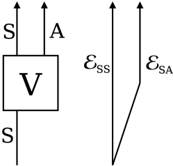
Figure 1: Interaction between a system $S$ and an apparatus $A$ of known initial state. Tracing over one of the two final system gives us one of two channels $\mathcal{E}_{SS}$ or $\mathcal{E}_{SA}$.

We can also trace out the final state of the system to get a channel from $\mathcal{L}(\mathcal{H}_{S})$ to $\mathcal{L}(\mathcal{H}_{A})$: $\mathcal{E}_{SA}(\rho)=\text{Tr}_{S}(V\rho V^{\dagger})$ where $\rho\in B(\mathcal{H}_{S})$. See Figure 1. The channel $\mathcal{E}_{SA}$ is uniquely defined by $\mathcal{E}_{SS}$, up to an arbitrary unitary operation on the apparatus, and is usually called the complementary channel of $\mathcal{E}_{SS}$. Its dual is simply

$$\mathcal{E}_{SA}^{\dagger}(Y)=V^{\dagger}({\bf 1}\otimes Y)V.$$

Using Theorem 9, we can determine which observables have been preserved by either $\mathcal{E}_{SS}$ or $\mathcal{E}_{SA}$, irrespectively of the system’s initial state. The answers are given by two subalgebras of $\mathcal{L}(\mathcal{H}_{S})$: respectively $\mathcal{A}_{SS}$ and $\mathcal{A}_{SA}$. The algebra $\mathcal{A}_{SS}$ characterizes the information about the system’s initial state which has been preserved by the system’s evolution, and $\mathcal{A}_{SA}$ characterizes the information about the system’s initial state which has been transferred to the environment.

Those algebras can be expressed in terms of the elements of one of the channels. For instance, if $E_{a}$ are elements for $\mathcal{E}_{SS}$, then $V$ can be expressed as $V=\sum_{b}E_{b}\otimes|\phi_{b}^{A}\rangle$ for some orthonormal set of vectors $|\phi_{b}^{A}\rangle$ of $\mathcal{H}_{A}$. Hence for any choice of a basis $|a\rangle$ of $\mathcal{H}_{S}$ we obtain a family of elements for the channel $\mathcal{E}_{SA}$, namely

$$F_{a}=\sum_{b}|\phi_{b}^{A}\rangle\langle a|E_{b}.$$

This means that the relevant operators entering Theorem 9 for the second channel are

$$F_{a}^{\dagger}F_{b}=\sum_{c}E_{c}^{\dagger}|a\rangle\langle b|E_{c}=\mathcal{E}_{SS}^{\dagger}(|a\rangle\langle b|).$$

Note that the operators $|a\rangle\langle b|$ form a basis for the whole operator algebra $\mathcal{L}(\mathcal{H}_{S})$. Hence the observables correctable for the apparatus form the algebra $\mathcal{A}_{SA}={\rm Alg}\bigl{(}{\rm Ran}\,\mathcal{E}_{SS}^{\dagger}\bigr{)}^{\prime}$: the algebra of operators commuting with all operators in the range of $\mathcal{E}_{SS}^{\dagger}$. Hence we see that a direct consequence of Theorem 9 is that in an open dynamics defined by a channel $\mathcal{E}$, full information about a projective observable can escape the system if and only if it commutes with the range of the dual map $\mathcal{E}^{\dagger}$, which is the set of observables with first moment information conserved by $\mathcal{E}$. This generalizes results in lindblad99 .

We can characterize the observables representing information which has been “duplicated” between the system and the apparatus. They form the intersection

$$\mathcal{C}:=\mathcal{A}_{SS}\cap\mathcal{A}_{SA}.$$

From the correctability of $\mathcal{A}_{SS}$ (Eq. (7)) we have that $\mathcal{A}_{SS}\subseteq{\rm Ran}\,\mathcal{E}_{SS}^{\dagger}$, from which it follows that ${\mathcal{A}}_{SA}={\rm Alg}\bigl{(}{\rm Ran}\,\mathcal{E}_{SS}^{\dagger}\bigr{)}^{\prime}\subseteq\mathcal{A}_{SS}^{\prime}$. Hence, the algebra of duplicated observables is $\mathcal{C}\subseteq\mathcal{A}_{SS}^{\prime}\cap\mathcal{A}_{SS}$, where $\mathcal{A}_{SS}^{\prime}\cap\mathcal{A}_{SS}$ is the center of $A_{SS}$: those elements of the algebra which commute with all other elements. In particular, the duplicated algebra $\mathcal{C}$ is commutative. Note that the contrary would have violated the no-cloning theorem after correction of both channels. Since the algebra $\mathcal{C}$ is commutative, it is generated by a single projective observable which can be represented by a self-adjoint operator $C$.

Given that, after the interaction, both the system and the apparatus contain information about the same observable $C$ on the initial state of the system, we may expect that they are correlated. Let $P_{i}\in\mathcal{C}$ be the projectors on the eigenspaces of $C$. There exists a POVM with elements $X_{i}$ on the system as well as a POVM $Y_{i}$ on the apparatus such that

$$\mathcal{E}^{\dagger}_{SS}(X_{i})=\mathcal{E}^{\dagger}_{SA}(Y_{i})=P_{i}.$$

Note that if $\mathcal{R}_{SS}$ and $\mathcal{R}_{SA}$ are correction channels for $\mathcal{E}_{SS}$ and respectively $\mathcal{E}_{SA}$, then $X_{i}=\mathcal{R}_{SS}^{\dagger}(P_{i})$ and $Y_{i}=\mathcal{R}_{SA}^{\dagger}(P_{i})$.

We will show that the observables $X_{i}$ and $Y_{i}$ are correlated. First note that $\text{Tr}(P_{i}P_{k})=\delta_{ki}$, which we can also write

$$\text{Tr}(P_{i}P_{k})=\text{Tr}(P_{i}\mathcal{E}^{\dagger}_{SS}(X_{k}))=\text{Tr}(P_{i}V^{\dagger}(X_{k}\otimes{\bf 1})V)=\delta_{ki}$$

This means that when $k\neq i$, $(X_{k}\otimes{\bf 1})VP_{i}=0$, which can be seen by expending $P_{i}$ in terms of eigenvectors. Also since $\sum_{k}X_{k}={\bf 1}$, then $VP_{i}=(X_{i}\otimes{\bf 1})VP_{i}$. The same argument is true also for $Y_{k}$. Therefore $(X_{k}\otimes{\bf 1})VP_{i}=({\bf 1}\otimes Y_{k})VP_{i}=\delta_{ik}VP_{i}$. Hence

$$\begin{split}V^{\dagger}(X_{i}\otimes Y_{j})V&=\sum_{kl}P_{k}V^{\dagger}(X_{i}\otimes Y_{j})VP_{l}=\sum_{kl}\delta_{ik}\delta_{jl}P_{i}P_{j}=\delta_{ij}P_{k}\end{split}$$

which means that for any state $\rho$ of the system

$$\text{Tr}(V\rho V^{\dagger}(X_{i}\otimes Y_{j}))=\delta_{ij}\text{Tr}(\rho P_{i}).$$

Hence the probability that the outcome of a measurement of $X$ differs from that of $Y$ is zero. This means that the information that the apparatus “learns” about the system and which is characterized by the observable $C$ is correlated with a property of the system after the interaction. Therefore $C$ represents the only information that the apparatus acquires about the system and which stays pertinent through the interaction.

This analysis has implication for the theory of decoherence giulini96 ; zurek03 as well as for the theory of measurements. We have shown that any interaction between a system and its environment (which took the role of the apparatus) automatically selects a unique observable $C$ as being the only predictive information about the system acquired by the environment. Even though an observer who has access to the environment could learn about any observable contained in the algebra $\mathcal{A}_{SA}$, only the information encoded by $C$ bears any information about the future state of the system. This suggests that the pointer states which characterize decoherence should not be selected only for their stability under the interaction with the environment: One should also add the requirement that they encode information that the environment learns about the system. Indeed any one of those requirements taken separately does not select a single observable unambiguously, but together they do. This is a new way of solving the basis ambiguity problem zurek81 .

V Error Correction of Operator Spaces

In this section we discuss an extension of OAQEC theory to the setting of operator spaces generated by observables. We shall leave a deeper analysis of this extension for investigation elsewhere. An operator space Pau02 is a linear manifold (a subspace) of operators inside $\mathcal{L}(\mathcal{H})$. Operator spaces, and their Hermitian closed counterpart “operator systems”, have arisen recently in the study of channel capacity problems in quantum information devetak05 . Observe that (by design) Definitions 3 and 8 include the case of operator spaces and systems generated by observables, and hence these cases fit into the mathematical framework for error correction introduced here. Let us describe how operator spaces physically arise in the present setting.

In Section III.1 we showed how to build the correction channel for active error correction. We were free to choose what to do to the system in the case that the syndrome measurement revealed the state had not initially been in the code prior to the action of the error channel. In fact, there is an advantage in choosing to send that state back in the code, meaning that we choose the correction channel such that $\mathcal{R}^{\dagger}(X)=\mathcal{R}^{\dagger}(PXP)$ for any operator $X$, which is indeed the case for the correction channel defined in Theorem 11. Consider the set of operators defined by

$$\mathcal{V}:=\mathcal{E}^{\dagger}(\mathcal{R}^{\dagger}(\mathcal{A})).$$

This set is not an algebra in general. Nevertheless, it is an operator system by the linearity and positivity of channels. If $X\in\mathcal{V}$ then there exists $Y\in P\mathcal{A}P$ such that $X=\mathcal{E}^{\dagger}(\mathcal{R}^{\dagger}(Y))$ and also $PXP=Y$. Therefore for all $X\in\mathcal{V}$,

$$\mathcal{E}^{\dagger}(\mathcal{R}^{\dagger}(X))=\mathcal{E}^{\dagger}(\mathcal{R}^{\dagger}(Y))=X.$$

Hence the observables in $\mathcal{V}$ are exactly corrected, and this is independent of what the initial state was. For instance, if we “forgot” to make sure that the initial state was in the code, we can still recover all the information, provided that we measure the observable with elements $X_{k}=\mathcal{E}^{\dagger}(\mathcal{R}^{\dagger}(Y_{k}))$ whenever we would have measured $Y_{k}\in\mathcal{A}$. Typically this would involve measuring general (unsharp) POVMs instead of just sharp projective observables. This shows that it could be useful to consider the correction of general POVMs. Since POVM elements do not always span an algebra, this suggests that we should consider the correctability (passive or active) codes associated with operator systems in this way.

Consider the following simple example of a conserved operator space that is not an algebra. Let $\mathcal{H}$ be single qutrit Hilbert space with computational basis $\{|0\rangle,|1\rangle,|2\rangle\}$. Consider the channel $\mathcal{E}$ on $\mathcal{H}$ defined by its action on observables represented in this basis as follows:

$$\mathcal{E}^{\dagger}\Big{(}[a_{ij}]_{3\times 3}\Big{)}\quad=\quad\left[\begin{matrix}a_{11}&a_{12}&0\\ a_{21}&a_{22}&0\\ 0&0&\frac{a_{11}+a_{22}}{2}\end{matrix}\right].$$ (12)

Observe that $(\mathcal{E}^{\dagger})^{2}=\mathcal{E}^{\dagger}\circ\mathcal{E}^{\dagger}=\mathcal{E}^{\dagger}$ and that the range $\mathcal{V}$ of $\mathcal{E}^{\dagger}$ coincides with its fixed point set; $\{Y:Y=\mathcal{E}^{\dagger}(X)\,\,{\rm for\,\,some\,\,}X\}=\{X:\mathcal{E}^{\dagger}(X)=X\}$. Thus, the operator system $\mathcal{V}$ is conserved by $\mathcal{E}$. Moreover, $\mathcal{V}$ is not an algebra since it is not closed under multiplication.

Given results from other settings for quantum error correction, it is of course desirable to find a characterization of correction for operator spaces independent of any particular recovery operation. Here we derive a necessary condition, and we leave the general question as an open problem. Observe that if there exists a channel $\mathcal{R}$ such that $P\mathcal{E}^{\dagger}(\mathcal{R}^{\dagger}(X))P=PXP$ for all $X\in\mathcal{V}$ then, $0\leq X\leq{\bf 1}$ implies $0\leq\mathcal{R}^{\dagger}(X)\leq{\bf 1}$, since $\mathcal{R}^{\dagger}$ is a contractive map. This in turn implies that there exists $0\leq Y\leq{\bf 1}$ such that $PXP=P\mathcal{E}^{\dagger}(Y)P$; namely, $Y=\mathcal{R}^{\dagger}(X)$.

Proposition 12.

A necessary condition for an operator space $V$ to be correctable on states $P\mathcal{H}$ for $\mathcal{E}$ is that for all $X\in\mathcal{V}$ such that $0\leq X\leq{\bf 1}$, there exists $0\leq Y\leq{\bf 1}$ such that $PXP=P\mathcal{E}^{\dagger}(Y)P$. This condition is also sufficient when $\mathcal{V}$ is an algebra containing $P$.

Proof. The first part of the statement has been proved. We show that the condition expressed implies correctability of $\mathcal{V}$ if it is an algebra containing $P$.

Since $P\in\mathcal{V}$, we know that $\mathcal{B}:=P\mathcal{V}P$ is a subalgebra of $\mathcal{V}$. Note it is sufficient to prove the correctability of $\mathcal{B}$. Indeed, if $\mathcal{B}$ is correctable then in particular $P$ is correctable. Let $\mathcal{R}$ be a correction channel for the largest correctable algebra on $P\mathcal{H}$. Then we have seen in the proof of Theorem 11 that the correctability of $P$ implies that $P\mathcal{E}^{\dagger}(\mathcal{R}^{\dagger}(X))P=P\mathcal{E}^{\dagger}(\mathcal{R}^{\dagger}(PXP))P$ for any $X$. From this it follows that the correctability of $\mathcal{B}$ on $P\mathcal{H}$ implies that of $\mathcal{V}$.

Let ${\mathbb{E}}:=\{X\;|\;0\leq X\leq{\bf 1}\}$. Suppose that $P\mathcal{(}V\cap{\mathbb{E}})P=\mathcal{B}\cap{\mathbb{E}}\subseteq P\mathcal{E}^{\dagger}({\mathbb{E}})P$. Then for all projectors $Q\in\mathcal{B}$, there exists a self-adjoint operator $0\leq X\leq{\bf 1}$ such that $P\mathcal{E}^{\dagger}(X)P=Q$. Hence $(P-Q)\mathcal{E}^{\dagger}(X)(P-Q)=0$, which implies $XE_{k}(P-Q)=0$, or $XE_{k}P=XE_{k}Q$ for all $k$. Also we have $P\mathcal{E}^{\dagger}({\bf 1}-X)P=P-Q$, so that $Q\mathcal{E}^{\dagger}({\bf 1}-X)Q=0$ from which $({\bf 1}-X)E_{k}Q=0$, or $E_{k}Q=XE_{k}Q$ for all $k$. Therefore

$$X(E_{k}P)=XE_{k}Q=E_{k}Q=(E_{k}P)Q.$$

Combining the two results we obtain

$$QPE_{k}^{\dagger}E_{j}P=PE_{k}^{\dagger}XE_{j}P=PE_{k}^{\dagger}E_{j}PQ$$

for all $k$ and all $j$. This result can linearly be extended to the whole of $\mathcal{B}$, since an algebra is spanned by its projectors. Hence $[X,PE_{k}^{\dagger}E_{j}P]=0$ for all $X\in\mathcal{B}$. From Theorem 11 this implies that $\mathcal{B}$, and therefore the algebra $\mathcal{V}$ is correctable on $P\mathcal{H}$. ∎

As a final example, consider the noise model corresponding to a single random bit flip on three qubits. The noise operators are $\{{\bf 1},X_{1},X_{2},X_{3}\}$ where $X_{i}$ is a Pauli $x$ matrix on the $i$th qubit. One can correct the standard quantum code with projector $P=|000\rangle\langle 000|+|111\rangle\langle 111|$ expressed in the computational basis. It is easy to check that a correction channel for this code is

$$\mathcal{R}^{\dagger}(A)=PAP+\sum_{i}X_{i}PAPX_{i}$$

This channel has the properties that we need in order to “lift” the code to an operator space code correctable on all states. Indeed, we have $\mathcal{R}^{\dagger}(P)={\bf 1}$ and $\mathcal{R}^{\dagger}(A)=\mathcal{R}^{\dagger}(PAP)$ for all $A$. The algebra correctable on the code $P$ is

$$\mathcal{A}=\Bigl{\{}\sum_{ij}\alpha_{ij}|iii\rangle\langle jjj|:\alpha_{ij}\in\mathbb{C}\Bigr{\}}$$

In order to proceed however we need a specific error channel, which is given by choosing a probability for the occurrence of each error:

$$\mathcal{E}(\rho)=p_{0}\rho+\sum_{i}p_{i}X_{i}\rho X_{i}$$

Then, writing $X_{0}={\bf 1}$, the operator space

$$\mathcal{V}=(\mathcal{R}\circ\mathcal{E})^{\dagger}(\mathcal{A})=\Bigl{\{}\sum_{i,j=0}^{1}\alpha_{ij}\sum_{k,l=0}^{3}p_{k}X_{k}X_{l}|iii\rangle\langle jjj|X_{l}X_{k}:\alpha_{ij}\in\mathbb{C}\Bigr{\}}$$

is correctable by $\mathcal{R}$ on all states. We should have $P\mathcal{V}P=\mathcal{A}$. This can be seen from the fact that $|iii\rangle=P|iii\rangle$ and $PX_{k}X_{l}P=\delta_{kl}P$. Explicitly separating the components respectively inside $\mathcal{A}$ and orthogonal to $\mathcal{A}$ we have operators in $\mathcal{V}$ which live in $\mathcal{A}$ and outside of $\mathcal{A}$:

$$\mathcal{V}=\Bigl{\{}\sum_{ij}\alpha_{ij}\Bigl{(}{|iii\rangle\langle jjj|+\sum_{k\neq l}p_{k}X_{k}X_{l}|iii\rangle\langle jjj|X_{l}X_{k}}\Bigr{)}:\alpha_{ij}\in\mathbb{C}\Bigr{\}}$$

Acknowledgements. We are grateful to the Banff International Research Station for kind hospitality. Some of the work for this paper took place during workshop 07w5119 on “Operator structures in quantum information theory”. This work was partially supported by NSERC, PREA, ERA, CFI, OIT, and the Canada Research Chairs program.

References

- (1) C. Bény, A. Kempf, and D. W. Kribs, Phys. Rev. Lett., 98, 100502 (2007).
- (2) C. H. Bennett, D. P. DiVincenzo, J. A. Smolin, and W. K. Wootters, Phys. Rev. A 54, 3824 (1996).
- (3) E. Knill and R. Laflamme, Phys. Rev. A 55, 900 (1997).
- (4) P. W. Shor, Phys. Rev. A 52, R2493 (1995).
- (5) A. M. Steane, Phys. Rev. Lett. 77, 793 (1996).
- (6) D. Gottesman, Phys. Rev. A 54, 1862 (1996).
- (7) D. Kribs, R. Laflamme, and D. Poulin, Phys. Rev. Lett. 94, 180501 (2005).
- (8) D. W. Kribs, R. Laflamme, D. Poulin, and M. Lesosky, Quant. Inf. & Comp. 6, 382 (2006).
- (9) G. Kuperberg, IEEE Trans. Inform. Theory 49, 1465 (2003).
- (10) M. A. Nielsen, and I. Chuang, Quantum computation and quantum information, Cambridge University Press (2000).
- (11) J. von Neumann, Mathematical foundations of quantum mechanics, Princeton University Press, Princeton, 1955.
- (12) K. R. Davidson, -algebras by example, Fields Institute Monographs, 6. American Mathematical Society, Providence, RI, 1996.
- (13) P. Zanardi and M. Rasetti, Phys. Rev. Lett. 79, 3306 (1997).
- (14) G. Palma, K.-A. Suominen, and A. Ekert, Proc. Royal Soc. A 452, 567 (1996).
- (15) L.-M. Duan and G.-C. Guo, Phys. Rev. Lett. 79, 1953 (1997).
- (16) D. A. Lidar, I. L. Chuang, and K. B. Whaley, Phys. Rev. Lett. 81, 2594 (1998).
- (17) E. Knill, R. Laflamme, and L. Viola, Phys. Rev. Lett. 84, 2525 (2000).
- (18) P. Zanardi, Phys. Rev. A 63, 12301 (2001).
- (19) J. Kempe, D. Bacon, D. A. Lidar, and K. B. Whaley, Phys. Rev. A 63, 42307 (2001).
- (20) M. Junge, P. Kim, and D. W. Kribs, J. Math. Phys. 46, 022102 (2005).
- (21) J.A. Holbrook, D.W. Kribs, R. Laflamme, and D. Poulin, Integral Eqtns. & Operator Thy., 51 (2005), 215-234.
- (22) J.A. Holbrook, D.W. Kribs, and R. Laflamme, Quant. Inf. Proc. 2, (2004), 381-419.
- (23) M.-D. Choi and D. W. Kribs, Phys. Rev. Lett. 96, 050501 (2006).
- (24) E. Knill, e-print quant-ph/0603252 (2006).
- (25) G. Lindblad, Lett. Math. Phys. 47, 189 (1999).
- (26) D. W. Kribs, Proc. Edin. Math. Soc. 46, 421 (2003).
- (27) E. Knill, R. Laflamme, A. Ashikhmin, H. Barnum, L. Viola, W. H. Zurek, LA Science 27, 188 (2002).
- (28) M. A. Nielsen and D. Poulin, e-print quant-ph/0506069 (2005).
- (29) D. Giulini et al., Decoherence and the Appearance of a Classical World in Quantum Theory (Springer, Berlin, 1996).
- (30) W. H. Zurek, Rev. Mod. Phys. 75, 715 (2003).
- (31) W. H. Zurek, Phys. Rev. D 24, 1516 (1981).
- (32) V. Paulsen, Completely bounded maps and operator algebras, Cambridge University Press, Cambridge, United Kingdom, 2002.
- (33) I. Devetak, M. Junge, C. King, and M. B. Ruskai, Comm. Math. Phys., 266 (2006), 37-63.