Cs CPT magnetometer for cardio-signal detection in unshielded environment

Abstract

We present first, encouraging results obtained with an experimental apparatus based on Coherent Population Trapping and aimed at detecting biological (cardiac) magnetic field in magnetically compensated, but unshielded volume. The work includes magnetic-field and magnetic-field-gradient compensation and uses differential detection for cancellation of (common mode) magnetic noise. Synchronous data acquisition with a reference (electro-cardiographic or pulse-oximetric) signal allows for improving the S/N in an off-line averaging. The set-up has the relevant advantages of working at room temperature with a small-size head, and of allowing for fast adjustments of the dc bias magnetic field, which results in making the sensor suitable for detecting the bio-magnetic signal at any orientation with respect to the heart axis and in any position around the patient chest, which is not the case with other kinds of magnetometers.

I Introduction

Spectroscopy of transitions involving long-lived levels in alkali atoms has shown impressive potentialities in the field of high resolution and high sensitivity magnetometry since the birth of coherent spectroscopy Blo62 ; Cohen69 ; Bud06 . In the last years, many research groups, with different experimental techniques like non linear magneto-optical rotationbudk_rev02 , spin-exchange relaxation free - Faraday rotation romalisSERF , double resonance optical pumping Groe06 , and Coherent Population Trapping (CPT) Kna02 ; NOI have obtained important records in optical magnetometry sensitivity, so to prove that atomic magnetometers are presently competitive even with SQUID magnetometers in terms of sensitivity, and can find applications in fields like geomagnetism monitoring, testing of materials, testing of fundamental symmetries of Physics and bio-magnetism detection.

The first mapping of the cardiomagnetic field with a Rubidium double resonance magnetometer has been demonstrated in ref.wei03a , and good agreement with the magnetocardiogram obtained by a SQUID magnetocardiograph has been foundwei03b .

The unique experiment of M. Romalis and coworkers Xia06 , recently showed that laser magnetometers can perform records in registration of such weak (few hundreds fT) magnetic fields as those produced by the human brain activity.

A fundamental request for actually reaching the sensitivity level needed for bio-signal detection is to reduce dramatically the environmental magnetic field. Usually high magnetic permeability materials like $\mu$-metal are employed to build small volumes inside of which it is possible to have very effective shielding of the external, undesired magnetic fields.

The high cost of such magnetically clean chambers represents a strong limitation for the diffusion of high sensitive magnetometry in clinical application, also because of their delicateness and possible magnetization with consequent requirement of periodical demagnetizing treatments.

The main limits of working in unshielded environmental conditions, typical in a scientific laboratory, are given by the presence of strong magnetic field gradients, ac magnetic fields in the volume of sensor cell and by the magnetic noise produced by other human activities and ionospheric phenomena.

Field gradients affect the sensitivity limit of the instrument by introducing a broadening of the detected resonance line. Time-dependent magnetic fields represent a further additional source limiting the magnetic field detection sensitivity.

The possibility of achieving high sensitivity, simply by passively quenching magnetic noise (placing thick Al plates around the magnetic sensor), has been shown in ref.seltz04 . There a sensitivity of the order of $1\rm{pT}/\sqrt{\rm{Hz}}$ is obtained thanks to a sophisticated feedback system that, keeping around zero the total magnetic field value in the volume of a K cell (heated to $170^{\circ}C$), suppresses the broadening due to spin-exchange-collisions.

In the present work, we show that a cheap system for eliminating spatial inhomogeneities of the background magnetic field, joined to an accurately balanced differential detection scheme, allows for detecting the magnetic signal produced by the heart activity without the use of neither expensive and bulky shielding chambers nor aluminum shields that attenuate high-frequency magnetic noise. The device consists in a full optical sensor operating at room temperature, placed inside a frame of compensation coils that can be easily accessed by a human body.

II Basics of the measurement principle

Magnetic field optical detection is performed by creating CPTNOI ; And03 on Zeeman sublevels of the F=3 hyperfine ground state of Cs atoms.

This is an all optical technique as it does not require the presence of coils in the proximity of the sensor cell in order to produce direct RF magnetic excitation. This feature makes easy to optimize the sensitivity to any orientation of the magnetic field, thus allowing for measuring any component of it. CPT is produced when circularly polarized laser radiation, resonant with a $\rm{D}_{2}$ optical transition, is frequency modulated exactly at the Zeeman frequency splitting of the ground Zeeman sublevels. The CPT signal can be seen as a resonant decrement of the absorption in the optical transition. The measure of the resonant frequency $\omega_{L}$ gives directly an absolute measurement of the modulus of the magnetic field interacting with the atomic probe.

This kind of magnetic field measurement is absolute and self-calibrated because the magnetic field strength $B$ is given by: $B=\frac{\omega_{L}}{\mu_{0}g_{F}}$, where $\mu_{0}$ is the Bohr magneton, $g_{F}$ is the Landé factor of the considered ground-state and $\omega_{L}$ is the resonance (Larmor) frequency. The magnetometer is a scalar one and the estimation of the magnetic field modulus is obtained by scaling the Larmor frequency by atomic constants, and only minor deviations may occur Wyn99 , introducing small systematic errors. Long time living coherence between Zeeman sublevels allows for creating very narrow (few Hz) resonances and then for getting very sensitive magnetic field estimations. Cs optical transitions can be excited by means of diode laser radiation, that can be easily modulated in frequency by means of the modulation of its injection current. Magnetic field intensities in the geophysical range, correspond to frequency modulations of the order of 100 kHz. This gives the possibility of performing high precision magnetic field measurement while operating in the presence of the local Earth magnetic field, by employing RF modulation of the laser currentbudk_mod_02 ; Aco06 ; NOI .

The presented experimental investigation is dedicated to the detection of a small, time varying field in the presence of about $10^{6}$ times stronger dc bias field, for any relative orientation of the two fields. As any scalar magnetometer, our setup is sensitive to the component of the varying magnetic field in the direction of the bias field (see also Section IV.1).

III Sensor set-up

The sensor set-up is sketched in Fig.1. Laser source is a single-mode edge-emitting pigtail laser ($\lambda$= 852 nm) with 15 mW of laser power and an intrinsic line-width of less than 5 MHz. Laser light is coupled to a single-mode polarization-maintaining fiber 10 m in length and the laser head, containing the laser chip, a 40 dB optical isolator, the temperature stability system (Peltier junction and the thermistor), and the fiber collimator is contained into a compact butterfly housing of $\mbox{4}0~{}\textrm{cm}^{3}$.

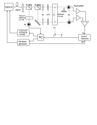
Figure 1: Experimental setup. PMOF: polarization maintaining optical fiber, CL:collimating lens, IBS: intensity beam splitter, NF: neutral filters, PD: photodiode.

The beam exiting from the fiber is collimated then split by an intensity beam splitter (IBS1). The beam reflected by IBS1 passes trough a vacuum reference cell and the transmitted light is detected in order to monitor the laser frequency tuning with respect to the Doppler line. The beam transmitted trough IBS1 is split again by a second intensity beam splitter IBS2. The beam reflected by IBS2 is made parallel to the transmitted one after reflection on a mirror M and plays the role of a second arm of the sensor. The two arms interaxial separation $\Delta$ is chosen to be about 7 cm. The polarization of both the beams is adjusted by means of two $\lambda/4$ plates. Both beams cross, in different points, a single cell, containing Cs and 5 Torr of $Ar$ as a buffer gas. The use of a single cylindrical cell, 9 cm in length and 1.5 cm in radius guarantees equal conditions for CPT creation (equal Cs and Ar vapor density in the two laser-atoms interaction volumes). All the component represented in Fig.1 are mounted on a non magnetic plate and the overall dimensions of the sensor are $25\times 12\times 4$ $\rm{cm}^{3}$.

In order to reduce power broadening, laser power is reduced to less than $50~{}\mbox{$\mu W$}$ in each sensor arm using a set of neutral filters. A non magnetic translating blade is placed after the cell, in front of one (the most sensitive) of the two photo-diodes, in order to have the possibility of fine balancing the detected photo-currents.

In order to increase the signal to noise ratio of the detected signal, phase sensitive detection is used. At this aim, we impose a 20 kHz frequency modulation on the RF frequency modulating the laser current and then detect the component of the signal oscillating at this frequency.

IV Sensitivity optimization for cardio-signal detection

The magnetic field produced by a human heart is characterized by a maximum intensity of about 100 pT in the close vicinity of the chest, and the main features are well reconstructed if sampled in a bandwidth of at least 30 Hz wei03a .

Magnetic heart-beat spatially confined distribution, of the order of the heart dimensions, allows for performing differential detection in a rather small volume in front of the patient’s chest, while the possibility of triggering the acquisition on other signal, taken for example from the electro-cardiogram (or even from a simple pulse oximeter), allows for effective noise rejection in an off-line analysis.

As introduced before, unshielded environmental conditions limit the instrumental sensitivity essentially because of the temporal and spatial fluctuation of the background magnetic field. Field gradients in our laboratory have the typical magnitude of about 100 $\rm{nT}/\rm{cm}$ depending on the presence of magnetic material both in the instrumentation and in the building structure. Alternating magnetic fields contribute instead, mainly with $50~{}\rm{Hz}$ and higher odd order harmonics, with a typical rms amplitude of the order of 100 nT depending on the vicinity of electric lines and power supply transformers. For frequencies higher than the lock-in cut-off frequency, ac fields determine an effective broadening of the CPT line, while for lower frequencies they directly introduce time fluctuation of the CPT resonance center. Optimization of the magnetometer sensitivity is fundamentally performed on the basis of the spatial and temporal characteristics of the bio-signal to be measured.

In order to improve the common mode noise rejection it is important to have, in absence of the magnetic source to be measured, exactly the same resonance profile at the two inputs of the differential lock-in amplifier. As shown in Ref.Kna02 small differences in laser power, polarization, beam-size contribute significantly to the unbalance by changing the amplitude and the shape (mainly) of the CPT resonance. Difference between the magnetic field values inside the two laser-atom interaction volumes shifts instead the positions of the resonances centers.

The cardiac signal measurement procedure consists in, first, adjustment of amplitude and width of the CPT signals in the two arms separately (single input mode of the lock-in amplifier) and, second, fine optimization of those parameters by looking at the maximum common mode noise cancellation in the differential signal (differential input mode of the lock-in amplifier).

IV.1 Field inhomogeneities compensation

As mentioned in Section II, measuring the modulus of $B$ in the presence of a strong dc component, leads to detect only the variations $\Delta B$ of the field in the component parallel to the dc, bias field since $\Delta\left|\vec{B}\right|\simeq\frac{\vec{B}}{\left|\vec{B}\right|}\cdot\Delta\vec{B}$.

By zeroing two of the three spatial component of the local background magnetic field, one is able to measure one selected component of the signal produced by the biological source. This gives the possibility of studying the different components of the measured field and eventually reconstructing the entire vectorial signal.

The typical configuration for a cardio-signal detection measurement is sketched in Fig.2. In this particular configuration both $x$ and $y$ components of the laboratory magnetic field are compensated (the residual magnetic field is in the 0.1 ${\rm{\mu}T}$ range) and thus, the $z$ component of the human heart magnetic beat is being detected.

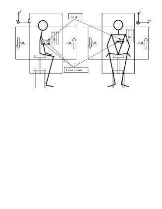
Figure 2: Schematics of the apparatus. The selected component of the background bias field $B_{0}$, parallel to $\hat{z}$ in the scheme, determines the direction of the detected component of the bio-signal, while laser beams separated by $\Delta$ are directed along $\hat{x}$. Dipoles are used for gradients compensation.

This detection scheme has important advantages in view of simplifying the compensation of magnetic field inhomogeneities. As explained in deeper detail in the Appendix, in fact, only 3 currents for the compensation of the spatial gradients inside the cell volume, are needed in addiction to the 2 currents employed for the zeroing of two of the three component of the laboratory magnetic field. These three currents flow respectively in one anti-Helmholtz pair and in two small coils playing the role of magnetic dipoles.

After the optimization of the gradient compensation we get a strong reduction of the line broadening due to magnetic field inhomogeneities. Fig. 3 shows the CPT resonance signal registered with and without the compensation of spatial gradients. Without compensation a best fit analysis gives a linewidth (FWHM) of about 1.7 kHz which is reduced down to less than 300 Hz in case of gradients compensation.

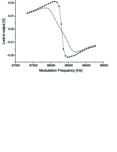
Figure 3: CPT line-shapes produced with circular polarization and magnetic field orientation orthogonal to the laser beam (along $\widehat{z}$ direction). Circles: static gradients are not compensated. Fitted line-width is 1.67 kHz. Squares: optimized compensation of the gradient components. Fitted line-width is reduced to 280 Hz.

IV.2 Differential measurement procedure and noise characterization

Depending on the spatial configuration of the local magnetic field in correspondence of the two light-atoms interaction volumes, we are able to cancel different noise contributions at the cost of increasing the uncorrelated electronic noise in the detection stage by namely a factor of $\sqrt{2}$. Other noise sources, like laser frequency noise and amplitude noise are systematically canceled from the signal provided that the two arms are balanced. If, furthermore, both arms of the sensor give CPT resonance exactly at the same resonant frequency, then even the common mode magnetic field noise, generated for example by all far magnetic sources is eliminated.

In Fig. 4 is presented the magnetometric noise spectral density for different operating conditions of the device. Trace (a) is relative to a single arm operation: laser noise and magnetic common mode noise contribute entirely. Trace (b) is obtained in differential input acquisition, where the two CPT resonances occur at frequencies separated by more than the CPT linewidth. In this case one mainly gets the cancellation of the laser frequency and intensity noise. Evident gain in the reduction of residual noise is obtained in the differential acquisition when CPT resonances detected by the two sensors are accurately overlapped (trace (c)). Trace (d) and (e) are recorded respectively in differential and single input mode, when the laser frequency is tuned out of the single photon (Doppler) resonance. It is evident that the uncorrelated electronic noise increases in the differential detection.

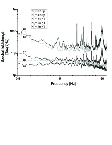
Figure 4: a) Single input acquisition: laser frequency is tuned to the center of the CPT resonance. b) Differential input acquisition: CPT signals on the two arms of the sensor are separated by more than the CPT linewidth. c) Differential input acquisition: CPT signals overlapping is optimized. d) Out of Doppler absorption resonance noise in differential input mode. e) Out of Doppler absorption resonance noise in single input mode. In the inset is reported the total rms noise $N$ integrated betweeen 1 Hz and 30 Hz (cardio-signal bandwidth) relative to each trace.

V Cardio signal data analysis

The signal-to-noise (S/N) ratio is not high enough to make single cardiac pulse directly observable, so that off-line analysis must include both linear filtration and averaging of the data. We use a standard technique for acquiring a reference signal simultaneously with the magnetometric data. Our digital lock-in amplifier (Stanford SR830) allows for storing up to 16384 data in a buffer, which can be synchronously acquired using an external clock. Thus we use an external DAQ card (MCC 1608FS, 16 bit resolution, with USB interface) whose ADC operation triggers the lock-in data storage. Such DAQ is used to sample reference data produced by either the pulse-oximeter or an electrocardiographic connection.

In the case of the pulse-oximeter, we arranged an IR led and a phototransistor in such a way to sense the transparency variation of a finger, and give several hundred mV signal peak-to-peak. Alternatively, the ECG was performed by acquiring digitally the electric signal collected by two electrodes placed in the vicinity of the heart, after a passive low-pass filtering, necessary to reduce the noise aliasing. Specifically, as we use typically a 128 S/s acquisition rate, a 18 dB/oct filter made with a three-stage RC cutting at 40 Hz, produced a clean signal about 1 mV at the QRS complex.

In both cases, the reference signal needs some preliminary (off-line) numerical conditioning before being used as a trigger. Namely, some linear filtering is performed to remove slow drifts and high frequency noise (a 3rd order bandpass numerical filter from 0.2 Hz to 30 Hz is usually suitable). After this, the envelope of the reference is evaluated, and used to normalize the peak-to-peak amplitude all along the registration. Finally, the normalized reference is used to produce a trigger signal which is adjustable in slope, threshold and hold-off, similarly to standard oscilloscopes. Additionally, and in particular when using pulse-oximeter reference, it is important to adjust a (negative) trigger delay, of some tenths of second, due to the relevant lag between the heart pulse and the change on the finger transparency. Both references showed to be suitable for data average triggering.

The magnetocardiographic data downloaded from the lock-in data buffer are firstly numerically filtered with the aim of removing specific spectral components (such as 50 Hz noise) and other spectral peaks due to artifacts (such as mechanical vibration of the Helmholtz coils) then split in traces corresponding to single heart pulses, from which the average pulse can be reconstructed by averaging.

The averaging process is not straightforward, due to the fact that the pulse duration is not stable. We tried two different approaches to superpose and average the single-pulse traces. In the first one, we strengthen the arrays containing the single pulse traces to a given size by linear interpolation, to make all of them equal in length; while in the second procedure we add zeros at the end of the shorter arrays to make all of them as long as the longest one. It turns out that the second procedure is more effective and correct, due to the fact that (as can be seen also by the ECG traces) the traces corresponding to single pulse cardiac activity are not similar to each other.

Specifically, each trace starts with a P-QRS-T complex having a pretty stable duration, followed by a quiescent interval whose duration is rather variable in time, which is the main responsible for the non-periodicity of the signal. As a consequence, using ECG reference, one finds that the averaging is the best (and the best is the S/N obtained) when triggering on the QRS complex (the highest peak) with a delay suitable to include the P wave of the same beat, while the location where the quiescent phase is being cut is not relevant, provided that the T wave of the previous beat is not included. In the case of pulse-oximeter as a reference the correct trigger delay must be found empirically due to its intrinsic additional delay.

In Fig. 5 is reported a reconstructed magnetic heart-beat, obtained by placing the sensor close to the chest of one of the authors. The peak is obtained from a data set consisting in 16384 points acquired at a sampling rate of 128 Hz. Average is thus performed on a set of about 150 heart-beats, corresponding to 128 sec of measuring time.

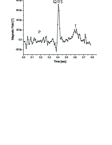
Figure 5: Reconstructed cardiac pulse. The signal is averaged over a set of about 150 cardiac pulses acquired at 128 Hz sampling rate. The lock-in equivalent noise band-width is 41.7  Hz.

VI Conclusions

We have demonstrated the potential of a fully optical, CPT based, differential magnetometers for magneto-cardiographic applications in unshielded environment, using a sample of Cs vapor at room temperature in a compact sensor head. We discussed simple approaches for magnetic-field and magnetic-field-gradient compensation, as well as off-line data analysis of quasi-periodic signals. The noise characterization showed that a severe limitation to the sensitivity would be set by the background magnetic field fluctuation, which, thanks to its essential uniformity can be effectively canceled in differential measurements. Specific features of the presented magnetometer, compared to others used at present lie in the facts that it works at room temperature and can be fast adjusted to detect different components of the weak biologic magnetic field vector, as the sensor, being purely optical, does not include coils, which would constitute geometrical constraints. The simplicity of the method, its low cost and low maintenance cost can be a crucial factor for its dissemination in clinical applications.

Magnetic-field and gradient compensation

In this appendix, we report the principles of the strategy for the resonance narrowing, shown in Fig. 3, obtained by means of magnetic field and magnetic field gradient conditioning.

In order to be able to independently compensate each of the three components of the magnetic field vector, while introducing minimum inhomogeneities, it is straightforward to use three pairs of coils in Helmholtz configuration (which for squared coils means to place them at a distance of about 0.544 L, L being the length of the coil side).

The center of the Cs vapor cell, the core of the optical sensor, is then placed at the geometrical center of a ”cube” composed by a set of three pairs of squared ($180\times 180\,\rm{cm}^{2}$) coils ($180\times 0.544$ is just enough to make possible a human body to access the cube).

Basic arguments give that not only $\vec{\nabla}\cdot\vec{B}$, but also $\vec{\nabla}\times\vec{B}$ is zero in the position of the sensor, as no current flows there. As a direct consequence, only five out of the nine elements of the matrix $\partial B_{i}/\partial x_{j}$ are independent, i.e. only five parameters have to be controlled for their compensation. More precisely, a complete compensation requires to controll two of the three diagonal elements, and three of the six off-diagonal elements.

The diagonal elements can be compensated by anti-Helmholtz coils. This means that two additional couples of coils with counter-propagating currents could be used to compensate $\partial B_{x}/\partial x$ and $\partial B_{y}/\partial y$ (which would guarantee also the compensation of $\partial B_{z}/\partial z$). In principle, such anti-Helmholtz coils should be at a larger distance, in order to produce the linear term $\partial B_{i}/\partial x_{i}$ and not the cubic one. But for simplicity, considering the small corrections to be made, is preferable to use the already existing Helmholtz pairs (with which, by the way, one has also the advantage of producing a maximum gradient, given the current).

This choice leads to simultaneously compensate the $x$ and $y$ components of the field and the three diagonal components of the gradient, by separately controlling the currents in the four Helmholtz coils for $B_{x}$ and $B_{y}$ compensation. Specifically, indicating with $I_{x1}$ and $I_{x2}$ the currents in the coils around the $x$ axis, $B_{x}$ is controlled by $(I_{x1}+I_{x2})$ and $\partial B_{x}/\partial x$ is controlled by $(I_{x1}-I_{x2})$ (similarly for the y direction). If only $B_{x}$ and $B_{y}$ are to be compensated, so that only $B_{z}$ inhomogeneities are relevant a simpler control can be made with three currents only, using pure Helmholtz configuration in $x$ and $y$ directions ($(I_{x1}=I_{x2})$, $(I_{y1}=I_{y2})$), and pure anti-Helmholtz $(I_{z1}=-I_{z2})$ configuration in the $z$ direction. In our present set-up, we opted for this latter, simpler choice.

The three independent off-diagonal elements of the gradient ($\partial B_{y}/\partial x$, $\partial B_{z}/\partial x$, $\partial B_{z}/\partial y$) can be controlled with couples of magnetic dipoles symmetrically located far away from the sensor in order to produce a vanishing, quadrupole field in the region of the cell. Again, provided that $\partial B_{y}/\partial x$ produces negligible effects because not responsible for $B_{z}$ inhomogeneities, only two of these three couples needs to be effectively adjusted. We actually use dipoles oriented in $z$ direction and located in the $xy$ plane. As the dipole field gradient decreases with the fourth power of the distance, fixing the dipoles on the frame of the large Helmholtz coils would make necessary to use pretty large current and pretty heavy coils. We simplified our task by using several couples of Nd permanent magnets in order to coarsely compensate the off-diagonal gradient components, and smaller electromagnets with few hundreds mA current for fine adjustments.

- (1) A. L. Bloom, ”Principles of operation of the rubidium vapor magnetometer”, Appl. Opt. 1, 61-68 (1962).
- (2) J. Dupont-Roc, S. Haroche, and C. Cohen-Tannoudji, ”Detection of very weak magnetic fields (10-9 Gauss) by 87Rb-zero-field level crossing resonances”, Phys. Lett. 28A, 638-639 (1969).
- (3) D. Budker and M. Romalis, ”Optical Magnetometry”, arXiv:physics/0611246v1 26Nov2006.
- (4) D. Budker, W. Gawlik, D. F. Kimball, M. Rochester, V. V. Yashchuk, and A. Weis, ”Resonant nonlinear magneto-optical effect in atoms” Rev.Mod.Phys. 74, 1154-1210 (2002).
- (5) J. Allred, R. Lyman, T. Kornack, M. Romalis. ”A high-sensitivity atomic magnetometer unaffected by spin-exchange relaxation.” PRL 89, 130801 (2002).
- (6) S. Groeger, G. Bison, J.-L. Schenker, R. Wynands and A. Weis, ”A high-sensitivity laser-pumped magnetometer”, European Phys. Jour. D 38, 239-247 (2006).
- (7) C. Affolderbach, M. Stahler, S. Knappe, R. Wynands, ”An all-optical, high-sensitivity magnetic gradiometer”, Appl.Phys. B 75, 605-612 (2002).
- (8) J. Belfi, G. Bevilacqua, V. Biancalana, Y. Dancheva, and L. Moi ”All optical sensor for automated magnetometry based on coherent population trapping”, Josa B (July 2007, in press).
- (9) G. Bison, R. Wynands, and A. Weis, ”A laser-pumped magnetometer for the mapping of human cardio-magnetic fields”, Appl.Phys. B 76, 325-328 (2003).
- (10) G. Bison, R. Wynands, and A. Weis, ”Dynamical mapping of the human cardiomagnetic field with a room-temperature, laser-optical sensor”, Optics Exp. 11, 904-909 (2003).
- (11) H. Xia, A. Ben-Amar Baranga, D. Hoffman, and M. V. Romalis, ”Magnetoencephalography with an atomic magnetometer”, Appl.Phys.Lett. 89, 211104 (2006).
- (12) S. J. Seltzer and M. Romalis, ”Unshielded three axis vector operation of a spin-exchange-relaxation-free atomic magnetometer”, Appl.Phys.Lett. 85, 4804-4806 (2004).
- (13) Ch. Andreeva, G. Bevilacqua, V. Biancalana, S. Cartaleva, Y. Dancheva, T. Karaulanov, C. Marinelli, E. Mariotti, and L. Moi, ”Two-color coherent population trapping in a single Cs hyperfine transition, with application in magnetometry”, Appl.Phys. B 76, 667-675 (2003).
- (14) R. Wynands and A. Nagel, ”Precision spectroscopy with coherent dark states”, Appl.Phys. B 68, 1-25 (1999).
- (15) D. Budker, D. F. Kimball, V. V. Yashchuk, and M. Zolotorev, ”Nonlinear magneto-optical rotation with frequency-modulated light”, PRA 65, 055403 (2002).
- (16) V. Acosta, M. P. Ledbetter, S. M. Rochester, and D. Budker, ”Nonlinear magneto-optical rotation with frequency-modulated light in the geophysical field range”, PRA 73, 053404 (2006).