Design of a Three-Axis Isotropic Parallel Manipulator for Machining Applications: The Orthoglide

Abstract

The orthoglide is a 3-DOF parallel mechanism designed at IRCCyN for machining applications. It features three fixed parallel linear joints which are mounted orthogonally and a mobile platform which moves in the Cartesian $x$-$y$-$z$ space with fixed orientation. The orthoglide has been designed as function of a prescribed Cartesian workspace with prescribed kinetostatic performances. The interesting features of the orthoglide are a regular Cartesian workspace shape, uniform performances in all directions and good compactness. A small-scale prototype of the orthoglide under development is presented at the end of this paper.

1 Introduction

Parallel kinematic machines (PKM) are interesting alternative designs for high-speed machining applications and have been attracting the interest of more and more researchers and companies. Since the first prototype presented in 1994 during the IMTS in Chicago by Gidding&Lewis (the Variax), many other prototypes have appeared.

However, the existing PKM suffer from two major drawbacks, namely, a complex Cartesian workspace and highly non linear input/output relations. For most PKM, the Jacobian matrix which relates the joint rates to the output velocities is not constant and not isotropic. Consequently, the performances (e.g. maximum speeds, forces accuracy and rigidity) vary considerably for different points in the Cartesian workspace and for different directions at one given point. This is a serious drawback for machining applications (Kim (1997); Treib et al. (1998); Wenger et al. (1999)). To be of interest for machining applications, a PKM should preserve good workspace properties, that is, regular shape and acceptable kinetostatic performances throughout. In milling applications, the machining conditions must remain constant along the whole tool path (Rehsteiner (1999); Rehsteiner et al. (1999)). In many research papers, this criterion is not taking into account in the algorithmic methods used for the optimization of the workspace volume (Luh et al. (1996); Merlet (1999)).

The orthoglide optimization is conducted to define a $3$-axis PKM with the advantages a classical serial PPP machine tool but not its drawbacks. Most industrial 3-axis machine-tool have a serial PPP kinematic architecture with orthogonal linear joint axes along the x, y and z directions. Thus, the motion of the tool in any of these directions is linearly related to the motion of one of the three actuated axes. Also, the performances are constant in the most part of the Cartesian workspace, which is a parallelepiped. The main drawback is inherent to the serial arrangement of the links, namely, poor dynamic performances.

The orthoglide is a PKM with three fixed linear joints mounted orthogonally. The mobile platform is connected to the linear joints by three articulated parallelograms and moves in the Cartesian x-y-z space with fixed orientation. Its workspace shape is close to a cube whose sides are parallel to the planes $xy$, $yz$ and $xz$ respectively. The optimization is conducted on the basis of the size of a prescribed cubic workspace with bounded velocity and force transmission factors. Two criteria are used for the architecture optimization of the orthoglide, (i) the conditioning of the Jacobian matrix of the PKM (Golub et al. (1989); Salisbury et al. (1982); Angeles (1997)) and (ii) the manipulability ellipsoid (Yoshikawa (1985)).

The first criterion leads to an isotropic architecture and to homogeneous performances in the workspace. The second criterion permits to optimize the actuated joint limits and the link lengths of the orthoglide with respect to the aforementioned two criteria.

Next section presents the orthoglide. The kinematic equations and the singularity analysis is detailed in Section 3. Section 4 is devoted to the optimization process of the orthoglide and to the presentation of the prototype.

2 Description of the Orthoglide

Most existing PKM can be classified into two main families. The PKM of the first family have fixed foot points and variable length struts and are generally called “hexapods”. They have a Stewart-Gought parallel kinematic architecture. Many prototypes and commercial hexapod PKM already exist like the Variax-Hexacenter (Gidding&Lewis), the CMW300 (Compagnie Mécanique des Vosges), the TORNADO 2000 (Hexel), the MIKROMAT 6X (Mikromat/IWU), the hexapod OKUMA (Okuma), the hexapod G500 (GEODETIC). In this first family, we find also hybrid architectures with a 2-axis wrist mounted in series to a 3-DOF tripod positioning structure (the TRICEPT from Neos Robotics).

The second family of PKM has been more recently investigated. In this category we find the HEXAGLIDE (ETH Zürich) which features six parallel (also in the geometrical sense) and coplanar linear joints. The HexaM (Toyoda) is another example with non coplanar linear joints. A 3-axis translational version of the hexaglide is the TRIGLIDE (Mikron), which has three coplanar and parallel linear joints. Another 3-axis translational PKM is proposed by the ISW Uni Stuttgart with the LINAPOD. This PKM has three vertical (non coplanar) linear joints. The URANE SX (Renault Automation) and the QUICKSTEP (Krause & Mauser) are 3-axis PKM with three non coplanar horizontal linear joints. The SPRINT Z3 (DS Technology) is a 3-axis PKM with one degree of translation and two degrees of rotations. A hybrid parallel/serial PKM with three parallel inclined linear joints and a two-axis wrist is the GEORGE V (IFW Uni Hanover).

PKMs of the second family are more interesting because the actuators are fixed and thus the moving masses are lower than in the hexapods and tripods.

The orthoglide presented in this article is a $3$-axis translational parallel kinematic machine with variable foot points and fixed length struts. Figure 2 shows the general kinematic architecture of the orthoglide.

The orthoglide has three parallel $PRPaR$ identical chains (where $P$, $R$ and $Pa$ stands for Prismatic, Revolute and Parallelogram joint, respectively). The actuated joints are the three orthogonal linear joints. These joints can be actuated by means of linear motors or by conventional rotary motors with ball screws. The output body is connected to the linear joints through a set of three parallelograms of equal lengths $L~{}=~{}B_{i}C_{i}$, so that it can move only in translation. The first linear joint axis is parallel to the $x$-axis, the second one is parallel to the $y$-axis and the third one is parallel to the $z$-axis. In figure 2, the base points $A_{1}$, $A_{2}$ and $A_{3}$ are fixed on the $i^{th}$ linear axis such that $A_{1}A_{2}=~{}A_{1}A_{3}=~{}A_{2}A_{3}$, $B_{i}$ is at the intersection of the first revolute axis ${\bf{i}}_{i}$ and the second revolute axis ${\bf{j}}_{i}$ of the $i^{th}$ parallelogram, and $C_{i}$ is at the intersection of the last two revolute joints of the $i^{th}$ parallelogram. When each $B_{i}C_{i}$ is aligned with the linear joint axis $A_{i}B_{i}$ , the orthoglide is in an isotropic configuration (see  4.4) and the tool center point $P$ is located at the intersection of the three linear joint axes. In this configuration, the base points $A_{1}$, $A_{2}$ and $A_{3}$ are equally distant from $P$. The symmetric design and the simplicity of the kinematic chains (all joints have only one degree of freedom, Fig. 2) should contribute to lower the manufacturing cost of the orthoglide.

The orthoglide is free of singularities and self-collisions. The workspace has a regular, quasi-cubic shape. The input/output equations are simple and the velocity transmission factors are equal to one along the $x$, $y$ and $z$ direction at the isotropic configuration, like in a serial $PPP$ machine (Wenger et al. (2000)).

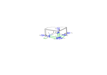
Figure 1: Orthoglide kinematic architecture

Figure 2: Leg kinematics

3 Kinematic Equations and Singularity Analysis

3.1 Static Equations

Let $\theta_{i}$ and $\beta_{i}$ denote the joint angles of the parallelogram about the axes ${\bf{i}}_{i}$ and ${\bf{j}}_{i}$, respectively (fig. 2). Let ${\bf{\rho}}_{1}$, ${\bf{\rho}}_{2}$, ${\bf{\rho}}_{3}$ denote the linear joint variables, ${\bf{\rho}}_{i}=A_{i}B_{i}$. In a reference frame (O, $x$, $y$, $z$) centered at the intersection of the three linear joint axes (note that the reference frame has been translated in Fig. 2 for more legibility) , the position vector p of the tool center point $P$ can be defined in three different ways:

$${\bf{p}}\!\! = \!\!\left[\begin{array}[]{c}a+\rho_{1}+\cos(\theta_{1})\cos(\beta_{1})L+e\\ \sin(\theta_{1})\cos(\beta_{1})L\\ -\sin(\beta_{1})L\end{array}\right]$$ (1d)

$${\bf{p}}\!\! = \!\!\left[\begin{array}[]{c}-\sin(\beta_{2})L\\ a+\rho_{2}+\cos(\theta_{2})\cos(\beta_{2})L+e\\ \sin(\theta_{2})\cos(\beta_{2})L\\ \end{array}\right]$$ (1h)

$${\bf{p}}\!\! = \!\!\left[\begin{array}[]{c}\sin(\theta_{3})\cos(\beta_{3})L\\ -\sin(\beta_{3})L\\ a+\rho_{3}+\cos(\theta_{3})\cos(\beta_{3})L+e\\ \end{array}\right]$$ (1l)

where $a=OA_{i}$, $e=C_{i}P$ and we recall that $L=B_{i}C_{i}$, ${\bf{\rho}}_{i}=A_{i}B_{i}$.

3.2 Kinematic Equations

Let $\dot{\mbox{\boldmath${\rho}$\unboldmath}}$ be referred to as the vector of actuated joint rates and $\dot{{\bf{p}}}$ as the velocity vector of point $P$:

$$\dot{\mbox{\boldmath${\rho}$\unboldmath}}=[\dot{\rho}_{1}~{}\dot{\rho}_{2}~{}\dot{\rho}_{3}]^{T},\quad\dot{{\bf{p}}}=[\dot{x}~{}\dot{y}~{}\dot{z}]^{T}$$

$\dot{{\bf{p}}}$ can be written in three different ways by traversing the three chains $A_{i}B_{i}C_{i}P$:

$$\dot{{\bf{p}}}\!\!\! = \!\!\!\!{\bf{n}}_{1}\dot{\rho}_{1}+(\dot{\theta}_{1}{\bf{i}}_{1}+\dot{\beta}_{1}{\bf{j}}_{1})\times({\bf{c}}_{1}-{\bf{b}}_{1})$$ (2a)

$$\dot{{\bf{p}}}\!\!\! = \!\!\!\!{\bf{n}}_{2}\dot{\rho}_{1}+(\dot{\theta}_{2}{\bf{i}}_{2}+\dot{\beta}_{2}{\bf{j}}_{2})\times({\bf{c}}_{2}-{\bf{b}}_{2})$$ (2b)

$$\dot{{\bf{p}}}\!\!\! = \!\!\!\!{\bf{n}}_{3}\dot{\rho}_{3}+(\dot{\theta}_{3}{\bf{i}}_{3}+\dot{\beta}_{3}{\bf{j}}_{3})\times({\bf{c}}_{3}-{\bf{b}}_{3})$$ (2c)

where ${\bf{b}}_{i}$ and ${\bf{c}}_{i}$ are the position vectors of the points $B_{i}$ and $C_{i}$, respectively, and ${\bf{n}}_{i}$ is the direction vector of the linear joints, for $i=1,2,$3.

3.3 Singular configurations

We want to eliminate the two idle joint rates $\dot{\theta}_{i}$ and $\dot{\beta}_{i}$ from Eqs. (2a–c), which we do upon dot-multiplying Eqs. (2a–c) by ${\bf{c}}_{i}-{\bf{b}}_{i}$:

$$({\bf{c}}_{1}-{\bf{b}}_{1})^{T}\dot{{\bf{p}}} = ({\bf{c}}_{1}-{\bf{b}}_{1})^{T}{\bf{n}}_{1}\dot{\rho}_{1}$$ (3a)

$$({\bf{c}}_{2}-{\bf{b}}_{2})^{T}\dot{{\bf{p}}} = ({\bf{c}}_{2}-{\bf{b}}_{2})^{T}{\bf{n}}_{2}\dot{\rho}_{2}$$ (3b)

$$({\bf{c}}_{3}-{\bf{b}}_{3})^{T}\dot{{\bf{p}}} = ({\bf{c}}_{3}-{\bf{b}}_{3})^{T}{\bf{n}}_{3}\dot{\rho}_{3}$$ (3c)

Equations (3a–c) can now be cast in vector form, namely

$${\bf{A}}\dot{\bf p}={\bf{B}}\dot{\mbox{\boldmath${\rho}$\unboldmath}}$$

where A and B are the parallel and serial Jacobian matrices, respectively:

$${\bf{A}}=\left[\begin{array}[]{c}({\bf{c}}_{1}-{\bf{b}}_{1})^{T}\\ ({\bf{c}}_{2}-{\bf{b}}_{2})^{T}\\ ({\bf{c}}_{3}-{\bf{b}}_{3})^{T}\end{array}\right]$$ (4d)

$${\bf{B}}=\left[\begin{array}[]{ccc}\eta_{1}&0&0\\ 0&\eta_{2}&0\\ 0&0&\eta_{3}\end{array}\right]$$ (4h)

with $\eta_{i}=({\bf{c}}_{i}-{\bf{b}}_{i})^{T}{\bf{n}}_{i}$ for $i=1,2,3$.

The parallel singularities (Chablat et al. (1998)) occur when the determinant of the matrix A vanishes, i.e. when $det({\bf{A}})=0$. In such configurations, it is possible to move locally the mobile platform whereas the actuated joints are locked. These singularities are particularly undesirable because the structure cannot resist any force. Eq. (4a) shows that the parallel singularities occur when:

$$({\bf{c}}_{1}-{\bf{b}}_{1})=\alpha({\bf{c}}_{2}-{\bf{b}}_{2})+\lambda({\bf{c}}_{3}-{\bf{b}}_{3})$$

that is when the points $B_{1}$, $C_{1}$, $B_{2}$, $C_{2}$, $B_{3}$ and $C_{3}$ are coplanar (Fig. 4). A particular case occurs when the links $B_{i}C_{i}$ are parallel (Fig. 4):

$$({\bf{c}}_{1}-{\bf{b}}_{1}) // ({\bf{c}}_{2}-{\bf{b}}_{2})\quad{\rm and}$$

$$({\bf{c}}_{2}-{\bf{b}}_{2}) // ({\bf{c}}_{3}-{\bf{b}}_{3})\quad{\rm and}$$

$$({\bf{c}}_{3}-{\bf{b}}_{3}) // ({\bf{c}}_{1}-{\bf{b}}_{1})$$

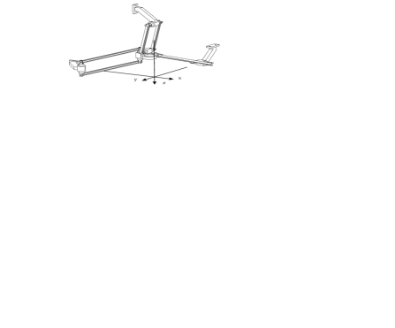
Figure 3: Parallel singular configuration when $B_{i}C_{i}$ are coplanar

Figure 4: Parallel singular configuration when $B_{i}C_{i}$ are parallel

Serial singularities arise when the serial Jacobian matrix B is no longer invertible i.e. when $det({\bf{B}})=0$. At a serial singularity a direction exists along which any cartesian velocity cannot be produced. Eq. (4b) shows that $\det({\bf{B}})=0$ when for one leg $i$, $({\bf{b}}_{i}-{\bf{a}}_{i})\perp({\bf{c}}_{i}-{\bf{b}}_{i})$.

The optimization of the orthoglide will put the serial and parallel singularities far away from the workspace (see  4.4).

4 Design and Performance Analysis of the Orthoglide

For usual machine tools, the Cartesian workspace is generally given as a function of the size of a right-angled parallelepiped. Due to the symmetrical architecture of the orthoglide, the Cartesian workspace has a fairly regular shape in which it is possible to include a cube whose sides are parallel to the planes $xy$, $yz$ and $xz$ respectively (Fig. 6).

The aim of this section is to define the dimensions of the orthoglide as a function of the size $L_{Workspace}$ of a prescribed cubic workspace with bounded transmission factors. We first show that the orthogonal arrangement of the linear joints is justified by the condition on the isotropy and manipulability: we want the orthoglide to have an isotropic configuration with velocity and force transmission factors equal to one. Then, we impose that the transmission factors remain under prescribed bounds throughout the prescribed workspace and we deduce the link dimensions and the joint limits.

4.1 Condition Number and Isotropic Configuration

The Jacobian matrix is said to be isotropic when its condition number attains its minimum value of one (Angeles (1997)). The condition number of the Jacobian matrix is an interesting performance index which characterises the distortion of a unit ball under the transformation represented by the Jacobian matrix. The Jacobian matrix of a manipulator is used to relate (i) the joint rates and the Cartesian velocities, and (ii) the static load on the output link and the joint torques or forces. Thus, the condition number of the Jacobian matrix can be used to measure the uniformity of the distribution of the tool velocities and forces in the Cartesian workspace.

4.2 Isotropic Configuration of the Orthoglide

For parallel manipulators, it is more convenient to study the conditioning of the Jacobian matrix that is related to the inverse transformation, ${\bf{J}}^{-1}$. When B is not singular, ${\bf{J}}^{-1}$ is defined by:

$$\dot{\mbox{\boldmath${\rho}$\unboldmath}}={\bf{J}}^{-1}\dot{{\bf{p}}}{\rm~{}~{}with~{}~{}}{\bf{J}}^{-1}={\bf{B}}^{-1}{\bf{A}}$$

Thus:

$${\bf{J}}^{-1}=\left[\begin{array}[]{c}(1/\eta_{1})({\bf{c}}_{1}-{\bf{b}}_{1})^{T}\\ (1/\eta_{2})({\bf{c}}_{2}-{\bf{b}}_{2})^{T}\\ (1/\eta_{3})({\bf{c}}_{3}-{\bf{b}}_{3})^{T}\end{array}\right]$$ (8)

with $\eta_{i}=({\bf{c}}_{i}-{\bf{b}}_{i})^{T}{\bf{n}}_{i}$ for $i=1,2,3$.

The matrix ${\bf{J}}^{-1}$ is isotropic when ${\bf{J}}^{-1}{\bf{J}}^{-T}=\sigma^{2}{\bf{1}}_{3\times 3}$, where ${\bf{1}}_{3\times 3}$ is the $3\times 3$ identity matrix. Thus, we must have,

$$\frac{1}{\eta_{1}}||{\bf{c}}_{1}-{\bf{b}}_{1}||=\frac{1}{\eta_{2}}||{\bf{c}}_{2}-{\bf{b}}_{2}||=\frac{1}{\eta_{3}}||{\bf{c}}_{3}-{\bf{b}}_{3}||$$ (9a)

$$({\bf{c}}_{1}-{\bf{b}}_{1})^{T}({\bf{c}}_{2}-{\bf{b}}_{2})=0$$ (9b)

$$({\bf{c}}_{2}-{\bf{b}}_{2})^{T}({\bf{c}}_{3}-{\bf{b}}_{3})=0$$ (9c)

$$({\bf{c}}_{3}-{\bf{b}}_{3})^{T}({\bf{c}}_{1}-{\bf{b}}_{1})=0$$ (9d)

Equation (9da) states that the orientation between the axis of the linear joint and the link $B_{i}C_{i}$ must be the same for each leg $i$. Equations (9db–d) mean that the links $B_{i}C_{i}$ must be orthogonal to each other. Figure 6 shows the isotropic configuration of the orthoglide. Note that the orthogonal arrangement of the linear joints is not a consequence of the isotropy condition, but it stems from the condition on the transmission factors at the isotropic configuration (see next section).

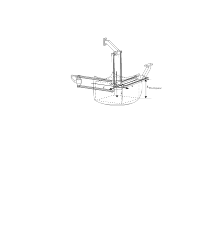
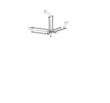
Figure 5: Cartesian workspace

Figure 6: Isotropic configuration of the Orthoglide mecanism

4.3 Manipulability Analysis

For a serial $PPP$ machine tool, Fig. 7, a motion of an actuated joint yields the same motion of the tool (the transmission factors are equal to one). In the purpose on our study, this factor is calculated from linear joint to the end-effector.

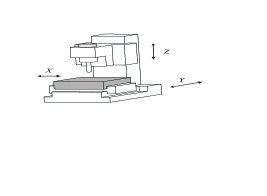
Figure 7: Typical industrial $3$-axis $PPP$ machine-tool

For a parallel machine, these motions are generally not equivalent. When the mechanism is close to a parallel singularity, a small joint rate can generate a large velocity of the tool. This means that the positioning accuracy of the tool is lower in some directions for some configurations close to parallel singularities because the encoder resolution is amplified. In addition, a velocity amplification in one direction is equivalent to a loss of rigidity in this direction.

The manipulability ellipsoids of the Jacobian matrix of robotic manipulators was defined several years ago (Salisbury et al. (1982)). This concept has then been applied as a performance index to parallel manipulators (Kim (1997)). Note that, although the concept of manipulability is close to the concept of condition number, these two concepts do not provide the same information. The condition number quantifies the proximity to an isotropic configuration, i.e. where the manipulability ellipsoid is a sphere, or, in other words, where the transmission factors are the same in all the directions, but it does not inform about the value of the transmission factor.

The manipulability ellipsoid of ${\bf{J}}^{-1}$ is used here for (i) justifying the orthogonal orientation of the linear joints and (ii) defining the joint limits of the orthoglide such that the transmission factors are bounded in the prescribed workspace.

We want the transmission factors to be equal to one at the isotropic configuration like for a $PPP$ machine tool. This condition implies that the three terms of Eq. (9d) must be equal to one:

$$\frac{1}{\eta_{1}}||{\bf{c}}_{1}-{\bf{b}}_{1}||=\frac{1}{\eta_{2}}||{\bf{c}}_{2}-{\bf{b}}_{2}||=\frac{1}{\eta_{3}}||{\bf{c}}_{3}-{\bf{b}}_{3}||=1$$ (10)

which implies that $({\bf{b}}_{i}-{\bf{a}}_{i})$ and $({\bf{c}}_{i}-{\bf{b}}_{i})$ must be collinear for each i.

Since, at this isotropic configuration, links $B_{i}C_{i}$ are orthogonal, Eq. (10) implies that the links $A_{i}B_{i}$ are orthogonal, i.e. the linear joints are orthogonal. For joint rates belonging to a unit ball, namely, $||\dot{\mbox{\boldmath${\rho}$\unboldmath}}||\leq 1$, the Cartesian velocities belong to an ellipsoid such that:

$$\dot{\mbox{\boldmath${p}$\unboldmath}}^{T}({\bf{J}}{\bf{J}}^{T})\dot{\mbox{\boldmath${p}$\unboldmath}}\leq 1$$

The eigenvectors of matrix $({\bf{J}}{\bf{J}}^{T})^{-1}$ define the direction of its principal axes of this ellipsoid and the square roots $\xi_{1}$, $\xi_{2}$ and $\xi_{3}$ of the eigenvalues of $({\bf{J}}{\bf{J}}^{T})^{-1}$ are the lengths of the aforementioned principal axes. The velocity transmission factors in the directions of the principal axes are defined by $\psi_{1}=1/\xi_{1}$, $\psi_{2}=1/\xi_{2}$ and $\psi_{3}=1/\xi_{3}$. To limit the variations of this factor in the Cartesian workspace, we impose

$$\psi_{min}\leq\psi_{i}\leq\psi_{max}$$ (11)

throughout the workspace. This condition determines the link lengths and the linear joint limits. To simplify the problem, we set $\psi_{min}=1/\psi_{max}$.

4.4 Design of the Orthoglide for a Prescribed Workspace

The aim of this section is to define the position of the fixed point $A_{i}$, the link lengths $L$ and the linear actuator range $\Delta\rho$ with respect to the limits on the transmission factors defined in Eq. (11) and as a function of the size of the prescribed workspace $L_{Workspace}$.

Our process of optimization is divided into three steps.

1. First, we determine two points $Q_{1}$ and $Q_{2}$ in the prescribed cubic workspace such that if the transmission factor bounds are satisfied at these points, they are satisfied in all the prescribed workspace.

2. The points $Q_{1}$ and $Q_{2}$ are used to define the leg length $L$ as function of the size of the prescribed cubic workspace.

3. Finally, the positions of the base points $A_{i}$ and the linear actuator range $\Delta\rho$ are calculated such that the prescribed cubic workspace is fully included in the Cartesian workspace of the orthoglide.

Step 1: The transmission factors are equal to one at the isotropic configuration. These factors increase or decrease when the tool center point moves away from the isotropic configuration and they tend towards zero or infinity in the vicinity of the singularity surfaces. It turns out that the points $Q_{1}$ and $Q_{2}$ defined at the intersection of the workspace boundary with the axis $x=y=z$ (figure 8) are the closest ones to the singularity surfaces, as illustrated in figure 9 which shows on the same top view the orthoglide in the two parallel singular configurations of figures  4 and  4. Thus, we may postulate the intuitive result that if the prescribed bounds on the transmission factors are satisfied at $Q_{1}$ and $Q_{2}$, then these bounds are satisfied throughout the prescribed cubic workspace. Although we could not derive a simple formal proof, we have verified numerically that this result holds.

Figure 8: Points $Q_{1}$ and $Q_{2}$

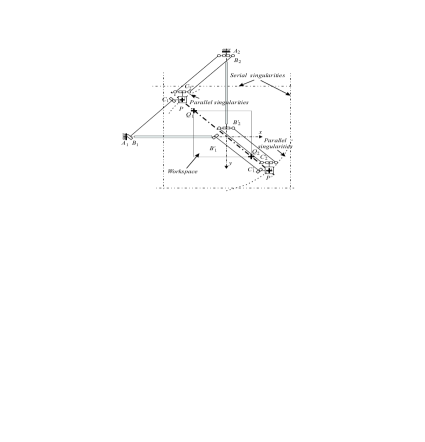
Figure 9: Points $Q_{1}$ and $Q_{2}$ and the singular configurations (top view)

Step 2: At the isotropic configuration, the angles $\theta_{i}$ and $\beta_{i}$ are equal to zero by definition. When the tool center point $P$ is at $Q_{1}$, $\rho_{1}=\rho_{2}=\rho_{3}=\rho_{min}$ (Fig. 10). When $P$ is at $Q_{2}$, $\rho_{1}=\rho_{2}=\rho_{3}=\rho_{max}$ (Fig. 11).

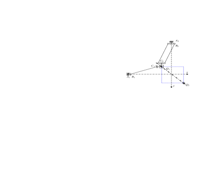
Figure 10: $Q_{1}$ configuration

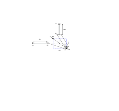
Figure 11: $Q_{2}$ configuration

We pose $\rho_{min}=0$ for more simplicity.

On the axis $(Q_{1}Q_{2})$, $\beta_{1}=\beta_{2}=\beta_{3}$ and $\theta_{1}=\theta_{2}=\theta_{3}$. We note,

$$\beta_{1}=\beta_{2}=\beta_{3}=\beta\quad{\rm and}\quad\theta_{1}=\theta_{2}=\theta_{3}=\theta$$ (12)

Upon substitution of Eq. (12) into Eqs. (1a–c), the angle $\beta$ can be written as a function of $\theta$,

$$\beta=-\arctan(\sin(\theta))$$ (13)

Finally, by substituting Eq. (13) into Eq. (8), the inverse Jacobian matrix ${\bf{J}}^{-1}$ can be simplified as follows

$${\bf{J}}^{-1}=\left[\begin{array}[]{ccc}1&-\tan(\theta)&-\tan(\theta)\\ -\tan(\theta)&1&-\tan(\theta)\\ -\tan(\theta)&-\tan(\theta)&1\end{array}\right]$$

Thus, the square roots of the eigenvalues of $({\bf{J}}{\bf{J}}^{T})^{-1}$ are,

$$\xi_{1}=|2\tan(\theta)-1|\quad{\rm and}\quad\xi_{2}=\xi_{3}=|\tan(\theta)+1|$$

And the three velocity transmission factors are,

$$\psi_{1}=\frac{1}{|2\tan(\theta)-1|}\quad{\rm and}\quad\psi_{2}=\psi_{3}=\frac{1}{|\tan(\theta)+1|}$$ (14)

Figure 12 depicts $\psi_{1}$, $\psi_{2}$ and $\psi_{3}$ as function of $\theta$ along the axis $(Q_{1}Q_{2})$.

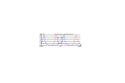
Figure 12: The three velocity transmission factors as function of $\theta$ along the axis $(Q_{1}Q_{2})$

The joint limits on $\theta$ are located on both sides of the isotropic configuration. To calculate the joint limits, we solve the following inequations,

$$\frac{1}{\psi_{max}}\leq\frac{1}{|2\tan(\theta)-1|}\leq\psi_{max}$$ (15a)

$$\frac{1}{\psi_{max}}\leq\frac{1}{|\tan(\theta)+1|}\leq\psi_{max}$$ (15b)

where the value of $\psi_{max}$ depends on the performance requirements. Two sets of joint limits ($[\theta_{Q_{1}}~{}\beta_{Q_{1}}]$ and $[\theta_{Q_{2}}~{}\beta_{Q_{2}}]$) are found. The detail of this calculation is given in the Appendix.

The position vectors ${\bf{q}}_{1}$ and ${\bf{q}}_{2}$ of the points $Q_{1}$ and $Q_{2}$, respectively, can be easily defined as a function of $L$ (Figs. 10 and 11),

$${\bf{q}}_{1}=[q_{1}~{}q_{1}~{}q_{1}]^{T}\quad{\rm and}\quad{\bf{q}}_{2}=[q_{2}~{}q_{2}~{}q_{2}]^{T}$$ (16a)

with

$$q_{1}=-\sin(\beta_{Q_{1}})L\quad{\rm and}\quad q_{2}=-\sin(\beta_{Q_{2}})L$$ (16b)

The size of the Cartesian workspace is,

$$L_{Workspace}=|q_{2}-q_{1}|$$

Thus, $L$ can be defined as a function of $L_{Workspace}$.

$$L=\frac{L_{Workspace}}{|\sin(\beta_{Q_{2}})-\sin(\beta_{Q_{1}})|}$$

Step 3: We want to determine the positions of the base points, namely, $a$. When the tool center point P is at $Q_{1}^{\prime}$ defined as the projection onto the $y$-axis of $Q_{1}$, $\rho=0$ and, (Fig. 13)

$$OA_{2}=OQ_{1}^{\prime}+Q_{1}^{\prime}C_{2}+C_{2}A_{2}$$

with $OA_{2}=a$, $OQ_{1}^{\prime}=q_{1}$, $Q_{1}^{\prime}C_{2}=PC_{2}=-e$ and since $\rho=0$, $C_{2}A_{2}=C_{2}B_{2}-L$. Thus,

$$a=q_{1}-e-L$$

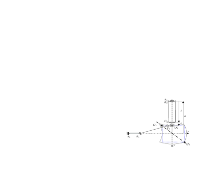
Figure 13: The point $Q_{1}^{\prime}$ used for the determination of $a$

Since $q_{1}$ is known from Eqs. (16a) and  (22b), $a$ can be calculated as function of $e$, $L$ and $\psi_{max}$.

Now, we have to calculate the linear joint range $\Delta\rho=\rho_{max}$ (we have posed $\rho_{min}$=0).

When the tool center point $P$ is at $Q_{2}$, $\rho=\rho_{max}$. The equation of the direct kinematics (Eq. (1b)) written at $Q_{2}$ yields,

$$\rho_{max}=q_{2}-a-\cos(\theta_{Q_{2}})\cos(\beta_{Q_{2}})L-e$$

4.5 Prototype

Using the aforementioned two kinetostatic criteria, a small-scale prototype is under development in our laboratory. The mechanical structure is now finished, (Fig. 14).

Figure 14: The orthoglide prototype

The actuated joints used for this prototype are rotative motors with ball screws. The prescribed performances of the orthoglide prototype are a Cartesian velocity of $1.2m/s$ and an acceleration of $14m/s^{2}$ at the isotropic point. The desired payload is $4kg$. The size of its prescribed cubic workspace is $200\times 200\times 200~{}mm$. We limit the variations of the velocity transmission factors as,

$$1/2\leq\psi_{i}\leq 2$$ (17)

The resulting length of the three parallelograms is $L=310~{}mm$ and the resulting range of the linear joints is $\Delta~{}\rho=~{}257~{}mm$. Thus, the ratio of the range of the actuated joints to the size of the prescribed Cartesian workspace is $r=200/257=0.78$. This ratio is high compared to other mechanisms. The three velocity transmission factors are depicted in Fig. 15. These factors are given in a $z$-cross section of the Cartesian workspace passing through $Q_{1}$.

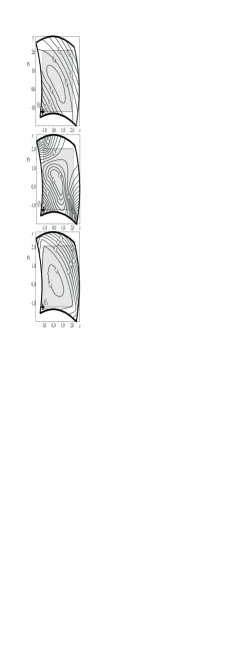
Figure 15: The three velocity transmission factors in a $z$-cross section of the Cartesian workspace passing through $Q_{1}$

5 Conclusions

Presented in this paper is a new kinematic structure of a PKM dedicated to machining applications: the Orthoglide. The main feature of this PKM design is its trade-off between the popular serial PPP architecture with homogeneous performances and the parallel kinematic architecture with good dynamic performances.

The workspace is simple, regular and free of singularities and self-collisions. The Jacobian matrix is isotropic at a point close to the center point of the workspace. Unlike most existing PKMs, the workspace is fairly regular and the performances are homogeneous in it. Thus, the entire workspace is really available for tool paths. In addition, the orthoglide is rather compact compared to most existing PKMs. A small-scale prototype of this mechanism is under construction at IRCCyN. First experiments with plastic parts will be conducted. The dynamic analysis has not been reported in this article. A rigid dynamic model has been proposed in (Guegan et al. (2002) and an elastic dynamic model is now being developed with the software package Meccano.

6 Appendix

To calculate the joint limits on $\theta$ and $\beta$, we solve the followings inequations, from the Eqs. 15,

$$|2\tan(\theta)-1|\leq\psi_{max}$$ (18a)

$$\frac{1}{|2\tan(\theta)-1|}\leq\psi_{max}$$ (18b)

Thus, we note,

$$f_{1}=|2\tan(\theta)-1|\quad f_{2}=1/|2\tan(\theta)-1|$$ (19a)

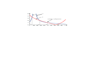
Figure 16: $f_{1}$ and $f_{2}$ as function of $\theta$ along $(Q_{1}Q_{2})$

Figure (16) shows $f_{1}$ and $f_{2}$ as function of $\theta$ along $(Q_{1}Q_{2})$. The four roots of $f_{1}=f_{2}$ in $[-\pi~{}\pi]$ are,

$$s_{1} = -\arctan\left((1+\sqrt{17})/4\right)$$ (20a)

$$s_{2} = -\arctan\left(1/2\right)$$ (20b)

$$s_{3} = 0$$ (20c)

$$s_{4} = \arctan\left((-1+\sqrt{17})/4\right)$$ (20d)

with

$$f_{1}(s_{1})=(-3+\sqrt{17})/4\quad f_{1}(s_{2})=2$$ (20e)

$$f_{1}(s_{3})=1\quad f_{1}(s_{4})=(3+\sqrt{17})/4$$ (20f)

and

$$f_{1}(\theta)=0 {\rm when} \theta=\arctan(1/2)-\pi$$ (21a)

$$f_{2}(\theta)=0 {\rm when} \theta=\arctan(1/2))$$ (21b)

The isotropic configuration is located at the configuration where $\theta=\beta=0$. The limits on $\theta$ and $\beta$ are in the vicinity of this configuration. Along the axis $(Q_{1}Q_{2})$, the angle $\theta$ is lower than $0$ when it is close to $Q_{2}$, and greater than $0$ when it is close to $Q_{1}$.

To find $\theta_{Q_{1}}$, we study the functions $f_{1}$ and $f_{2}$ which are both decreasing on $[0~{}\arctan(1/2)]$. Thus, we have,

$$\theta_{Q_{1}} = \arctan\left({\frac{{\psi_{max}}-1}{{2\psi_{max}}}}\right)$$ (22a)

$$\beta_{Q_{1}} = -\arctan\left({\frac{\psi_{max}-1}{\sqrt{5\psi_{max}^{2}-2\psi_{max}+1}}}\right)$$ (22b)

In the same way, to find $\theta_{Q_{2}}$, we study the functions $f_{1}$ and $f_{2}$ on $[s_{1}~{}0]$. The three roots $s_{1}$, $s_{2}$ and $s_{3}$ define two intervals. If $\psi_{max}\in[f_{1}(s_{1})~{}f_{1}(s_{2})]$, we have,

$$\theta_{Q_{2}} = -\arctan\left({\frac{{\psi_{max}}-1}{{\psi_{max}}}}\right)$$ (23a)

$$\beta_{Q_{2}} = \arctan\left({\frac{\psi_{max}-1}{\sqrt{2\psi_{max}^{2}-2\psi_{max}+1}}}\right)$$ (23b)

otherwise, if $$\psi_{max}\in[f_{1}(s_{2})~{}f_{1}(s_{3})]$$,

$$\theta_{Q_{2}} = -\arctan\left({\frac{\psi_{max}-1}{{2}}}\right)$$ (23c)

$$\beta_{Q_{2}} = \arctan\left({\frac{\psi_{max}-1}{\sqrt{{\psi_{max}}^{2}-2\psi_{max}+5}}}\right)$$ (23d)

References

- Treib et al. (1998) Treib, T. and Zirn, O. “Similarity laws of serial and parallel manipulators for machine tools”, Proc. Int. Seminar on Improving Machine Tool Performance, pp. 125–131, Vol. 1, 1998.
- Wenger et al. (1999) Wenger, P. Gosselin, C. and Maille. B. “A Comparative Study of Serial and Parallel Mechanism Topologies for Machine Tools”, Proc. PKM’99, Milano, pp. 23–32, 1999.
- Kim (1997) Kim J. , Park C., Kim J. and Park F.C., 1997, “Performance Analysis of Parallel Manipulator Architectures for CNC Machining Applications”, Proc. IMECE Symp. On Machine Tools, Dallas.
- Wenger et al. (1999) Wenger, P. Gosselin, C. and Chablat. D. “A Comparative Study of Parallel Kinematic Architectures for Machining Applications”, Proc. Workshop on Computational Kinematics’2001, Seoul, Korea, pp. 249–258, 2001.
- Rehsteiner (1999) Rehsteiner, F., Neugebauer, R.. Spiewak, S. and Wieland, F., 1999, “Putting Parallel Kinematics Machines (PKM) to Productive Work”, Annals of the CIRP, Vol. 48:1, pp. 345–350.
- Rehsteiner et al. (1999) Tlusty, J., Ziegert, J, and Ridgeway, S., 1999, “Fundamental Comparison of the Use of Serial and Parallel Kinematics for Machine Tools”, Annals of the CIRP, Vol. 48:1, pp. 351–356.
- Luh et al. (1996) Luh C-M., Adkins F. A., Haug E. J. and Qui C. C., 1996, “Working Capability Analysis of Stewart platforms”, Transactions of ASME, pp. 220–227.
- Merlet (1999) Merlet J-P., 1999, “Dertemination of 6D Workspace of Gough-Type Parallel Manipulator and Comparison between Different Geometries”, The Int. Journal of Robotic Research, Vol. 19, No. 9, pp. 902–916.
- Golub et al. (1989) Golub, G. H. and Van Loan, C. F., Matrix Computations, The John Hopkins University Press, Baltimore, 1989.
- Salisbury et al. (1982) Salisbury J-K. and Craig J-J., 1982, “Articulated Hands: Force Control and Kinematic Issues”, The Int. J. Robotics Res., Vol. 1, No. 1, pp. 4–17.
- Angeles (1997) Angeles J., 1997, Fundamentals of Robotic Mechanical Systems, Springer-Verlag.
- Yoshikawa (1985) Yoshikawa, T., “Manipulability of Robot Mechanisms”, 1985, The Int. J. Robotics Res., Vol. 4, No. 2, pp. 3–9.
- Wenger et al. (2000) Wenger, P., and Chablat, D., 2000, “Kinematic Analysis of a new Parallel Machine Tool: the Orthoglide”, in Lenarčič, J. and Stanišić, M.M. (editors), Advances in Robot Kinematic, Kluwer Academic Publishers, June, pp. 305–314.
- Chablat et al. (1998) Chablat D. and Wenger P., 1998, “Working Modes and Aspects in Fully-Parallel Manipulator”, IEEE Int. Conf. On Robotics and Automation, pp. 1964–1969.
- Guegan et al. (2002) Guegan S. and Khalil W., 2002, “Dynamic Modeling of the Orthoglide”, to appear in Advances in Robot Kinematic, Kluwer Academic Publishers, June.