Quark-lepton mass unification at TeV scales

Abstract

A scenario combining a model of early (TeV) unification of quarks and leptons with the physics of large extra dimensions provides a natural mechanism linking quark and lepton masses at TeV scale. This has been dubbed as early quark-lepton mass unification by one of us (PQH) in one of the two models of early quark-lepton unification, which are consistent with data, namely $\mathrm{SU}(4)_{\mathrm{PS}}\otimes\mathrm{SU}(2)_{L}\otimes\mathrm{SU}(2)_{R}\otimes\mathrm{SU}(2)_{H}$. In particular, it focused on the issue of naturally light Dirac neutrino. The present paper will focus on similar issues in the other model, namely $\mathrm{SU}(4)_{\mathrm{PS}}\otimes\mathrm{SU}(3)_{L}\otimes\mathrm{SU}(3)_{H}$.

I Introduction

Could quark and lepton masses be related at TeV scales? Not long ago, one of us explored this possibility in the framework of the so-called early quark-lepton mass unification Hung (2005). The idea was to combine two TeV scale scenarios, namely one of the two petite unification models $\mathrm{PUT}_{1}=\mathrm{SU}(4)_{\mathrm{PS}}\otimes\mathrm{SU}(2)_{L}\otimes\mathrm{SU}(2)_{R}\otimes\mathrm{SU}(2)_{H}$, and TeV scale large extra dimensions Antoniadis (1990); Arkani-Hamed et al. (1998).

The Petite Unification Theories (PUT’s) Hung et al. (1982); Buras and Hung (2003) are quark-lepton unification models, which occur at TeV scales and have the gauge group structure $G=G_{S}(g_{S})\otimes G_{W}(g_{W})$. Both PUT models propose unusually charged heavy quarks and leptons, in addition to the fermion content of the Standard Model (SM).

The model in Ref. Hung (2005) made use of the mechanism of wave function overlap along the large extra dimension Arkani-Hamed et al. (1998); Antoniadis et al. (1998), which was originally employed to justify the smallness of Dirac neutrino mass Arkani-Hamed and Schmaltz (2000); Hung (2003); Arkani-Hamed et al. (2001). The mechanism connects the strengths of the couplings in the mass terms of the fermions in four dimensions, as effective Yukawa couplings, to the magnitudes of wave function overlaps between the corresponding left- and right-handed fermionic zero modes along the large extra dimension Arkani-Hamed and Schmaltz (2000); Hung (2003).

In this framework, therefore, the shapes of the wave functions of left- and right-handed fermions plus distances between those wave functions in the extra dimension determine the strengths of the mass terms in four dimensions.

The geometry of the fermionic zero modes along the extra dimension was systematically set in Ref. Hung (2005) by breaking the symmetries of the model in the extra dimension down to that of the Standard Model, which was the approach originally suggested in Ref. Hung (2003). As a result, Ref. Hung (2005) obtained early quark-lepton mass unification, within which the four-dimensional (4D) Yukawa couplings of the chiral fermions of the model related to each other and a light Dirac neutrino was made possible.

The present work intends to build a model based on the marriage of the other petite unification model, ${\mathrm{PUT}}_{2}=\mathrm{SU}(4)_{\mathrm{PS}}\otimes\mathrm{SU}(3)_{L}\otimes\mathrm{SU}(3)_{H}$, and the physics of large extra dimension in the context of “brane world” picture, in order to explore its implications. Similar to the work in Ref. Hung (2005), we make use of the idea of wave function overlaps along the extra dimension and set the geometry of the zero modes by symmetry breakings.

Historically, questions on quark-lepton mass relation were addressed in a quark-lepton unification scenario, e.g., Grand Unified Theories (GUT’s) Georgi and Glashow (1974). A well-known example of this is the equality of $\tau$-lepton and bottom-quark masses Buras et al. (1978) at $M_{GUT}$ in $\mathrm{SU}(5)$ scenario. A TeV scale quark-lepton mass relation differs from a GUT one in the amount of “running” one needs to be concerned about if one attempts to explore the implications at lower energies, say $M_{Z}$.

On another front, the present work assumes a Dirac neutrino, which will turn out light in a direct correlation with the masses of heavy unconventional fermions. Such connection between a light Dirac neutrino and TeV-scale physics is in contrast with the traditional seesaw mechanism Gell-Mann et al. (1979), where its scale is limited perhaps only by Planck mass. Very recently, however, a TeV scale scenario for seesaw mechanism Hung (2007) has been put forward, which broadens the implications on TeV-scale physics to both Dirac and Majorana light neutrinos. Of course, the final word on the nature of neutrino, whether it is a Majorana or Dirac particle, must come from experiment, in particular those regarding lepton number violation.

The outline of the paper is as follows. First, we go over the idea of petite unification theories briefly followed by a review on the group structure and the particle content of $\mathrm{PUT}_{2}$ scenario. Then, we present a five dimensional model based on $\mathrm{PUT}_{2}$ scenario plus a short review on the wave function overlap mechanism. Afterward, we set the geometry of the zero mode wave functions of chiral fermions by systematic symmetry breakings in the extra dimension. In subsequent sections, we move toward the computation of chiral fermion mass scales by relating them to the magnitudes of applicable overlaps in the extra dimension. A numerical analysis concludes the mass scale computation, which substantiates the notion of early quark-lepton mass unification. Then, we examine the validity of our model by computing the electroweak oblique parameter $S$ and the lifetimes of heavy chiral fermions.

II Petite unification of quarks and leptons

Petite unification models Hung et al. (1982) were built around the idea of unifying quarks and leptons at an energy scale not too much higher than the electroweak scale. They have the gauge group structure of $G=G_{S}(g_{S})\otimes G_{W}(g_{W})$ with two independent couplings $g_{S}$ and $g_{W}$, which must contain the SM fields. The first PUT model was constructed based on the knowledge of the low-energy $\sin^{2}\theta_{W}$ value and known fermion representations at the time. With the $\mathrm{SU}(4)_{\mathrm{PS}}$ group of Pati and Salam Pati and Salam (1974) chosen for $G_{S}$ and the constraint from the experimental value of $\sin^{2}\theta_{W}(M_{Z}^{2})$, known at the time, the gauge group $\mathrm{PUT}_{0}=\mathrm{SU}(4)_{\mathrm{PS}}\otimes[\mathrm{SU}(2)]^{4}$ with unification scale of several hundreds of TeV emerged and was proposed in Ref. Hung et al. (1982).

Later precise measurements of $\sin^{2}\theta_{W}(M_{Z}^{2})$ plus renewed interest in TeV scale physics, however, resulted in a thorough re-examination of the PUT idea Buras and Hung (2003), yielding three favorable PUT models: $\mathrm{PUT}_{0}$ and $\mathrm{PUT}_{1,2}$, where

$${\mathrm{PUT}}_{1}=\mathrm{SU}(4)_{\mathrm{PS}}\otimes\mathrm{SU}(2)_{L}\otimes\mathrm{SU}(2)_{R}\otimes\mathrm{SU}(2)_{H},$$ (1)

and

$${\mathrm{PUT}}_{2}=\mathrm{SU}(4)_{\mathrm{PS}}\otimes\mathrm{SU}(3)_{L}\otimes\mathrm{SU}(3)_{H}.$$ (2)

The new measured value of $\sin^{2}\theta_{W}(M_{Z}^{2})$, which was higher than its old value, lowered the unification scale down to a few-TeV region. This lower scale rules out $\mathrm{PUT}_{0}$ scenario due to problems with the decay rate of $K_{L}\rightarrow\mu e$ at tree level. The remaining two models, $\mathrm{PUT}_{1}$ and $\mathrm{PUT}_{2}$, however, are found to naturally avoid the violation of the upper bound on the $K_{L}\rightarrow\mu e$ rate at tree level. The SM gauge group with three couplings, $\mathrm{SU}(3)_{c}(g_{3})\otimes\mathrm{SU}(2)_{L}(g_{2})\otimes\mathrm{U}(1)_{Y}(g_{1})$, is assumed to be embedded into the PUT groups with two couplings. The symmetry breaking scheme of PUT scenarios is given by

$$G\stackrel{{\scriptstyle\textstyle M}}{{\longrightarrow}}G_{1}\stackrel{{\scriptstyle\textstyle\tilde{M}}}{{\longrightarrow}}G_{2}\stackrel{{\scriptstyle\textstyle M_{Z}}}{{\longrightarrow}}\mathrm{SU}(3)_{c}\otimes\mathrm{U}(1)_{EM},$$ (3a)

where

$$G_{1}=\mathrm{SU}(3)_{c}(g_{3})\otimes\mathrm{U}(1)_{S}(\tilde{g}_{S})\otimes G_{W}(g_{W})\,,$$ (3b)

and

$$G_{2}=\mathrm{SU}(3)_{c}(g_{3})\otimes\mathrm{SU}(2)_{L}(g_{2})\otimes\mathrm{U}(1)_{Y}(g^{\prime})\ ,$$ (3c)

with $M_{Z}<\tilde{M}\leq M$. The two PUT scenarios have three new generations of unconventional quarks and leptons, in addition to the three standard generations of quarks and leptons. The magnitude of the charges of these new particles can reach up to $4/3$ (for “quarks”) and 2 (for “leptons”). The horizontal groups $\mathrm{SU}(2)_{H}$ and $\mathrm{SU}(3)_{H}$ connect the standard fermions to the unconventional ones, as well as the gauge bosons of $\mathrm{SU}(4)_{\mathrm{PS}}/\left[\mathrm{SU}(3)_{c}\otimes\mathrm{U}(1)_{S}\right]$.

In both PUT models the $\mathrm{SU}(4)_{\mathrm{PS}}$ quartets contain either “unconventional quark and the SM lepton” or “SM quark and unconventional lepton.” As a result, there is no tree-level transition between ordinary quarks and leptons mediated by the $\mathrm{SU}(4)_{\mathrm{PS}}/\left[\mathrm{SU}(3)_{c}\otimes\mathrm{U}(1)_{S}\right]$ gauge bosons. This important property prevents rare decays such as $K_{L}\rightarrow\mu e$ from acquiring large rates, since it can only occur through one-loop processes which can be made small enough to comply with the experimental bound.

Another property of PUT scenarios is the existence of new contributions to flavor changing neutral current (FCNC) processes, involving standard quarks and leptons, which are mediated by the horizontal $\mathrm{SU}(2)_{H}$ and $\mathrm{SU}(3)_{H}$ weak gauge bosons and the new unconventional quarks and leptons. Nonetheless, they appear at one-loop level and can be made consistent with the existing experimental bounds. A thorough analysis of $\mathrm{PUT}_{1}$ was carried out by the authors of Ref. Buras et al. (2004).

III $\text{PUT}_{2}$ model

In this scenario the weak gauge group is $G_{W}=\mathrm{SU}(3)_{L}\otimes\mathrm{SU}(3)_{H}$, where the SM’s $\mathrm{SU}(2)_{L}$ is the subgroup of its $\mathrm{SU}(3)_{L}$. The gauge symmetry breaking of $\mathrm{PUT}_{2}$ follows the scheme given in Eqs. (3).

Within such symmetry breaking, the strong $\mathrm{U}(1)_{S}$ group corresponds to the unbroken diagonal generator of $\mathrm{SU}(4)_{\mathrm{PS}}$, i.e., $\hat{Y}_{S}$. The weak hypercharge $\mathrm{U}(1)_{Y}$ group emerges from $\mathrm{U}(1)_{S}$ and $G_{W}$ breaking, whose generator $\hat{Y}_{W}$ can be written as $\hat{Y}_{W}=C_{S}\hat{T}_{15\mathrm{PS}}+C_{L}\hat{T}_{8L}+C_{1H}\hat{T}_{8H}+C_{2H}\hat{T}_{3H}$ where $\hat{T}$’s are the diagonal generators of $\tilde{G}_{S}$, $\mathrm{SU}(3)_{L}$ and $\mathrm{SU}(3)_{H}$ symmetries. The SM’s $\hat{T}_{3L}$ generator is simply the third generator of $\mathrm{SU}(3)_{L}$, which goes into the unbroken $\mathrm{SU}(2)_{L}$ subgroup. Note that this is all in the “unlocked standard model” picture of Ref. Hung et al. (1982), where the generators of $\mathrm{SU}(2)_{L}$ are the unbroken generators of $G_{W}$. The $C_{i}$ coefficients in $\hat{Y}_{W}$ define the embedment of the SM’s weak hypercharge group $\mathrm{U}(1)_{Y}$ into $G_{1}$.

The two symmetry breaking scales $M$ and $\tilde{M}$ were determined in Ref. Buras and Hung (2003) by renormalization group (RG) evolution combined with the very precise experimental value of $\sin^{2}\theta_{W}\left({M_{Z}^{2}}\right)$. The values could differ by up to an order of magnitude, roughly $3\leqslant M\leqslant 10{\text{ TeV}}$ and $0.8\leqslant\tilde{M}\leqslant 3{\text{ TeV}}$.

The charge operator in PUT scenarios is defined as $\hat{Q}=\hat{Q}_{W}+C_{S}\hat{T}_{15\mathrm{PS}}$, where $\hat{Q}_{W}$ is the weak charge given by $\hat{Q}_{W}=\hat{T}_{3L}+C_{L}\hat{T}_{8L}+C_{1H}\hat{T}_{8H}+C_{2H}\hat{T}_{3H}$. The weak charge $Q_{W}$, as shown in Ref. Hung et al. (1982), is related to $\sin^{2}\theta_{W}^{0}$ defining the charge distribution of the relevant representations of PUT scenarios. For $\mathrm{PUT}_{2}$ model, $C_{S}^{2}={8\mathord{\left/{\vphantom{83}}\right.\kern-1.2pt}3}$ and the important group theoretical factor $\sin^{2}\theta_{W}^{0}$ is given by $\sin^{2}\theta_{W}^{0}={1\mathord{\left/{\vphantom{1{\left({1+C_{W}^{2}}\right)}}}\right.\kern-1.2pt}{\left({1+C_{W}^{2}}\right)}}={3\mathord{\left/{\vphantom{38}}\right.\kern-1.2pt}8}$ , where $C_{W}^{2}=C_{L}^{2}+C_{1H}^{2}+C_{2H}^{2}={5\mathord{\left/{\vphantom{53}}\right.\kern-1.2pt}3}$.

For the model in question, the fermion representations, which together are anomaly-free, are $(4,3,\bar{3})$ and $(4,\bar{3},3)$. The charge distribution of the fermion content of $(4,3,\bar{3})$ representation is

$$\mathcal{Q}_{1}=\Biggl{(}{\left[{\left({\frac{1}{3},\frac{4}{3},\frac{4}{3}}\right),\left({-1,0,0}\right)}\right],\left[{\left({-\frac{2}{3},\frac{1}{3},\frac{1}{3}}\right),\left({-2,-1,-1}\right)}\right],\left[{\left({-\frac{2}{3},\frac{1}{3},\frac{1}{3}}\right),\left({-2,-1,-1}\right)}\right]}\Biggr{)}\,,$$ (4)

Similarly, for $(4,\bar{3},3)$ the charge distribution is given by

$$\mathcal{Q}_{2}=\Biggl{(}{\left[{\left({\frac{1}{3},-\frac{2}{3},-\frac{2}{3}}\right),\left({-1,-2,-2}\right)}\right],\left[{\left({\frac{4}{3},\frac{1}{3},\frac{1}{3}}\right),\left({0,-1,-1}\right)}\right],\left[{\left({\frac{4}{3},\frac{1}{3},\frac{1}{3}}\right),\left({0,-1,-1}\right)}\right]}\Biggr{)}\,,$$ (5)

In terms of $\mathrm{SU}(2)_{L}$ doublets and singlets, one can write $(4,3,\bar{3})$ as

$$\Psi_{1,L}=\Biggl{(}{\bigg{[}{\Big{(}{\bm{\psi}^{Q*},D^{c}}\Big{)},\Big{(}{\psi^{l},\nu^{c}}\Big{)}}\bigg{]},\bigg{[}{\Big{(}{\bm{\psi}^{q*},d^{c}}\Big{)},\Big{(}{\bm{\psi}^{L*},l_{d}^{c}}\Big{)}}\bigg{]},\bigg{[}{\Big{(}{\tilde{\bm{\psi}}^{q*},\tilde{\mathtt{d}}^{*}}\Big{)},\Big{(}{\tilde{\bm{\psi}}^{L*},\tilde{\mathtt{l}}^{*}}\Big{)}}\bigg{]}}\Biggr{)}_{L},$$ (6)

and $(4,\bar{3},3)$ as

$$\Psi_{2,L}=\Biggl{(}{\bigg{[}{\Big{(}{\tilde{\bm{\psi}}^{q,c},u^{c}}\Big{)},\Big{(}{\tilde{\bm{\psi}}^{L,c},l_{u}^{c}}\Big{)}}\bigg{]},\bigg{[}{\Big{(}{\tilde{\bm{\psi}}^{Q,c},U^{c}}\Big{)},\Big{(}{\tilde{\psi}^{l,c*},l^{c*}}\Big{)}}\bigg{]},\bigg{[}{\Big{(}{\tilde{\bm{\psi}}^{Q*},\tilde{\mathtt{d}}^{c}}\Big{)},\Big{(}{\tilde{\psi}^{l},\tilde{\mathtt{l}}^{c}}\Big{)}}\bigg{]}}\Bigg{)}_{L}.$$ (7)

Before we identify the $\mathrm{SU}(2)_{L}$ doublets and singlets appearing in Eqs. (6 and 7), let us first point out that in Eqs. (6 and 7) the right-handed fields are written in terms of the left-handed charge conjugates; so that the whole representation is left handed, e.g., $\nu_{L}^{c}$ or $u_{L}^{c}$. Besides, to match the charge distributions of Eqs. (4 and 5), some $\mathrm{SU}(2)_{L}$ doublets, in Eqs. (6 and 7), appear in italic-boldface typeset. To explain this notation, consider an arbitrary doublet

$$\psi_{L,R}=\left({\begin{array}[]{*{20}c}{\psi_{u}}\\ {\psi_{d}}\\ \end{array}}\right)_{L,R},$$ (8)

then $\bm{\psi}_{L,R}$, the rotated doublet in $\mathrm{SU}(2)$ space by $\pi$ about the second axis, is defined as

$$\bm{\psi}_{L,R}\equiv i\tau_{2}\psi_{L,R}=\left({\begin{array}[]{*{20}c}{\psi_{d}}\\ {-\psi_{u}}\\ \end{array}}\right)_{L,R}.$$ (9)

The $\mathrm{SU}(2)_{L}$ doublets and singlets present in $(4,3,\bar{3})$ are

$$\psi^{q}_{L}=\left(\begin{array}[]{c}u(2/3)\\ d(-1/3)\end{array}\right)_{L}\,;\,\,d^{c}_{L}(1/3)=C\bar{d}^{\,T}_{R}\,,$$ (10a)

$$\psi^{l}_{L}=\left(\begin{array}[]{c}\nu(0)\\ l(-1)\end{array}\right)_{L}\,;\,\,\nu^{c}_{L}=C\bar{\nu}_{R}^{T}\,,$$ (10b)

$$\psi^{Q}_{L}=\left(\begin{array}[]{c}U(-1/3)\\ D(-4/3)\end{array}\right)_{L}\,;\,\,D^{c}_{L}(4/3)=C\bar{D}^{T}_{R}\,,$$ (10c)

$$\psi^{L}_{L}=\left(\begin{array}[]{c}l_{u}(2)\\ l_{d}(1)\end{array}\right)_{L}\,;\,\,l^{c}_{d,L}(-1)=C\bar{l}^{\,T}_{d,R}\,,$$ (10d)

$$\tilde{\psi}^{L}_{L}=\left(\begin{array}[]{c}\tilde{l}_{u}(2)\\ \tilde{l}_{d}(1)\end{array}\right)_{L}\,;\,\,\tilde{\mathtt{l}}_{L}(+1)\,,$$ (10e)

$$\tilde{\psi}^{q}_{L}=\left(\begin{array}[]{c}\tilde{u}(2/3)\\ \tilde{d}(-1/3)\end{array}\right)_{L}\,;\,\,\tilde{\mathtt{d}}_{L}(-1/3)\,.$$ (10f)

In the above list, one notices normal quarks and leptons, and those with unusual electric charges. On the other hand, the $\mathrm{SU}(2)$ doublets and singlets of $(4,\bar{3},3)$ are

$$\tilde{\psi}^{l}_{L,R}=\left(\begin{array}[]{c}\tilde{\nu}(0)\\ \tilde{l}(-1)\end{array}\right)_{L,R}\,;\,\,\,l^{c}_{L}(+1)=C\bar{l}^{\,T}_{R}\,,$$ (11a)

$$\tilde{\mathtt{l}}_{R}(+1)\ \,;\ \,u_{L}^{c}\left({{{-2}\mathord{\left/{\vphantom{{-2}3}}\right.\kern-1.2pt}3}}\right)=C\bar{u}^{T}_{R}\,,$$ (11b)

$$\tilde{\psi}^{q}_{R}=\left(\begin{array}[]{c}\tilde{u}(+2/3)\\ \tilde{d}(-1/3)\end{array}\right)_{R}\ \,;\,\,\tilde{\mathtt{d}}_{R}(-1/3)\,,$$ (11c)

$$\tilde{\psi}^{L}_{R}=\left(\begin{array}[]{c}\tilde{l}_{u}(2)\\ \tilde{l}_{d}(1)\end{array}\right)_{R}\ \,;\,\,l^{c}_{u,L}(-2)=C\bar{l}^{\,T}_{u,R}\,,$$ (11d)

$$\tilde{\psi}^{Q}_{L,R}=\left(\begin{array}[]{c}\tilde{U}(-1/3)\\ \tilde{D}(-4/3)\end{array}\right)_{L,R}\ \,;\;\,U^{c}_{L}(1/3)=C\bar{U}^{T}_{R}\,.$$ (11e)

One notices two types of families with SM transformation property in both $\Psi_{1}$ and $\Psi_{2}$. This means left-handed doublets and right-handed singlets for each family. One family includes SM quarks and leptons (normal fermions) and the other contains unconventional quarks and leptons, i.e., those with unusual charges. These unconventional particles are $\psi^{Q}_{L}$, $D^{c}_{L}$, $U^{c}_{L}$, and $\psi^{L}_{L}$, $l^{c}_{d,L}$, $l^{c}_{u,L}$. The normal and unconventional quarks and leptons will receive mass through their couplings with the SM Higgs field.

In addition, the fermion content of $\mathrm{PUT}_{2}$ includes two vector-like $\mathrm{SU}(2)_{L}$ doublets of quarks and leptons $(\tilde{\psi}^{q},\tilde{\psi}^{l})_{L,R}$ and $(\tilde{\psi}^{Q},\tilde{\psi}^{L})_{L,R}$, with normal and unusual charges, and two vector-like $\mathrm{SU}(2)_{L}$ singlets $\tilde{\mathtt{l}}_{L,R}$ and $\tilde{\mathtt{d}}_{L,R}$. These vector-like particles can obtain large bare masses as mentioned in Ref. Buras and Hung (2003).

Let us write the two representations in terms of quartets and triplets of the corresponding gauge symmetry groups. For $\Psi_{1L}$, we have the following multiplets:

• $\mathrm{SU}(4)_{\mathrm{PS}}$ quartets

  $$\begin{array}[]{*{20}c}{\left({\begin{array}[]{*{20}c}{D^{*}_{L}\left({{4\mathord{\left/{\vphantom{43}}\right.\kern-1.2pt}3}}\right)}\\ {\nu_{L}\left(0\right)}\\ \end{array}}\right)}&;&{\left({\begin{array}[]{*{20}c}{-U^{*}_{L}\left({{1\mathord{\left/{\vphantom{13}}\right.\kern-1.2pt}3}}\right)}\\ {l_{L}\left({-1}\right)}\\ \end{array}}\right)}&;&{\left({\begin{array}[]{*{20}c}{D_{L}^{c}\left({{4\mathord{\left/{\vphantom{43}}\right.\kern-1.2pt}3}}\right)}\\ {\nu_{L}^{c}\left(0\right)}\\ \end{array}}\right)}\,,\\ \end{array}$$ (12a)

  $$\begin{array}[]{*{20}c}{\left({\begin{array}[]{*{20}c}{d^{*}_{L}\left({{1\mathord{\left/{\vphantom{13}}\right.\kern-1.2pt}3}}\right)}\\ {l^{*}_{d,L}\left({-1}\right)}\\ \end{array}}\right)}&;&{\left({\begin{array}[]{*{20}c}{-u^{*}_{L}\left({{{-2}\mathord{\left/{\vphantom{{-2}3}}\right.\kern-1.2pt}3}}\right)}\\ {-l^{*}_{u,L}\left({-2}\right)}\\ \end{array}}\right)}&;&{\left({\begin{array}[]{*{20}c}{d_{L}^{c}\left({{1\mathord{\left/{\vphantom{13}}\right.\kern-1.2pt}3}}\right)}\\ {l_{d,L}^{c}\left({-1}\right)}\\ \end{array}}\right)}\,,\\ \end{array}$$ (12b)

  $$\begin{array}[]{*{20}c}{\left({\begin{array}[]{*{20}c}{\tilde{d}^{*}_{L}\left({{{-2}\mathord{\left/{\vphantom{{-2}3}}\right.\kern-1.2pt}3}}\right)}\\ {\tilde{l}^{*}_{d,L}\left({-1}\right)}\\ \end{array}}\right)}&;&{\left({\begin{array}[]{*{20}c}{-\tilde{u}^{*}_{L}\left({{{-2}\mathord{\left/{\vphantom{{-2}3}}\right.\kern-1.2pt}3}}\right)}\\ {-\tilde{l}^{*}_{u,L}\left({-2}\right)}\\ \end{array}}\right)}&;&{\left({\begin{array}[]{*{20}c}{\tilde{\mathtt{d}}_{L}^{*}\left({{1\mathord{\left/{\vphantom{13}}\right.\kern-1.2pt}3}}\right)}\\ {\tilde{\mathtt{l}}_{L}^{*}\left({-1}\right)}\\ \end{array}}\right)}\,,\\ \end{array}$$ (12c)

• $\mathrm{SU}(3)_{L}$ triplets

  $$\begin{array}[]{*{20}c}{\left({\begin{array}[]{*{20}c}{D^{*}_{L}\left({{4\mathord{\left/{\vphantom{43}}\right.\kern-1.2pt}3}}\right)}\\ {-U^{*}_{L}\left({{1\mathord{\left/{\vphantom{13}}\right.\kern-1.2pt}3}}\right)}\\ {D_{L}^{c}\left({{4\mathord{\left/{\vphantom{43}}\right.\kern-1.2pt}3}}\right)}\\ \end{array}}\right)}&;&{\left({\begin{array}[]{*{20}c}{\nu_{L}\left(0\right)}\\ {l_{L}\left({-1}\right)}\\ {\nu_{L}^{c}\left(0\right)}\\ \end{array}}\right)}&;&{\left({\begin{array}[]{*{20}c}{d^{*}_{L}\left({{1\mathord{\left/{\vphantom{13}}\right.\kern-1.2pt}3}}\right)}\\ {-u^{*}_{L}\left({{{-2}\mathord{\left/{\vphantom{{-2}3}}\right.\kern-1.2pt}3}}\right)}\\ {d_{L}^{c}\left({{1\mathord{\left/{\vphantom{13}}\right.\kern-1.2pt}3}}\right)}\\ \end{array}}\right)}\,,\\ \end{array}$$ (13a)

  $$\begin{array}[]{*{20}c}{\left({\begin{array}[]{*{20}c}{l^{*}_{d,L}\left({-1}\right)}\\ {-l^{*}_{u,L}\left({-2}\right)}\\ {l_{d,L}^{c}\left({-1}\right)}\\ \end{array}}\right)}&;&{\left({\begin{array}[]{*{20}c}{\tilde{d}^{*}_{L}\left({{1\mathord{\left/{\vphantom{13}}\right.\kern-1.2pt}3}}\right)}\\ {-\tilde{u}^{*}_{L}\left({{{-2}\mathord{\left/{\vphantom{{-2}3}}\right.\kern-1.2pt}3}}\right)}\\ {\tilde{\mathtt{d}}_{L}^{*}\left({{1\mathord{\left/{\vphantom{13}}\right.\kern-1.2pt}3}}\right)}\\ \end{array}}\right)}&;&{\left({\begin{array}[]{*{20}c}{\tilde{l}^{*}_{d,L}\left({-1}\right)}\\ {-\tilde{l}^{*}_{u,L}\left({-2}\right)}\\ {\tilde{\mathtt{l}}_{L}^{*}\left({-1}\right)}\\ \end{array}}\right)}\,,\\ \end{array}$$ (13b)

• $\mathrm{SU}(3)_{H}$ antitriplets

  $$\begin{array}[]{*{20}c}{\left({\begin{array}[]{*{20}c}{d^{*}_{L}\left({{1\mathord{\left/{\vphantom{13}}\right.\kern-1.2pt}3}}\right)}\\ {D^{*}_{L}\left({{4\mathord{\left/{\vphantom{43}}\right.\kern-1.2pt}3}}\right)}\\ {\tilde{d}^{*}_{L}\left({{1\mathord{\left/{\vphantom{13}}\right.\kern-1.2pt}3}}\right)}\\ \end{array}}\right)}&;&{\left({\begin{array}[]{*{20}c}{-u^{*}_{L}\left({{{-2}\mathord{\left/{\vphantom{{-2}3}}\right.\kern-1.2pt}3}}\right)}\\ {-U^{*}_{L}\left({{1\mathord{\left/{\vphantom{13}}\right.\kern-1.2pt}3}}\right)}\\ {-\tilde{u}^{*}_{L}\left({{{-2}\mathord{\left/{\vphantom{{-2}3}}\right.\kern-1.2pt}3}}\right)}\\ \end{array}}\right)}&;&{\left({\begin{array}[]{*{20}c}{d_{L}^{c}\left({{1\mathord{\left/{\vphantom{13}}\right.\kern-1.2pt}3}}\right)}\\ {D_{L}^{c}\left({{4\mathord{\left/{\vphantom{43}}\right.\kern-1.2pt}3}}\right)}\\ {\tilde{\mathtt{d}}_{L}^{*}\left({{1\mathord{\left/{\vphantom{13}}\right.\kern-1.2pt}3}}\right)}\\ \end{array}}\right)}\,,\\ \end{array}$$ (14a)

  $$\begin{array}[]{*{20}c}{\left({\begin{array}[]{*{20}c}{l^{*}_{d,L}\left({-1}\right)}\\ {\nu_{L}\left(0\right)}\\ {\tilde{l}^{*}_{d,L}\left({-1}\right)}\\ \end{array}}\right)}&;&{\left({\begin{array}[]{*{20}c}{-l^{*}_{u,L}\left({-2}\right)}\\ {l_{L}\left({-1}\right)}\\ {-\tilde{l}^{*}_{u,L}\left({-2}\right)}\\ \end{array}}\right)}&;&{\left({\begin{array}[]{*{20}c}{l_{d,L}^{c}\left({-1}\right)}\\ {\nu_{L}^{c}\left(0\right)}\\ {\tilde{\mathtt{l}}_{L}^{*}\left({-1}\right)}\\ \end{array}}\right)}\,,\\ \end{array}$$ (14b)

For $\Psi_{2L}$, on the other hand, the corresponding multiplets are:

• $\mathrm{SU}(4)_{\mathrm{PS}}$ quartets

  $$\begin{array}[]{*{20}c}{\left({\begin{array}[]{*{20}c}{\tilde{d}_{L}^{c}\left({{1\mathord{\left/{\vphantom{13}}\right.\kern-1.2pt}3}}\right)}\\ {\tilde{l}_{d,L}^{c}\left({-1}\right)}\\ \end{array}}\right)}&;&{\left({\begin{array}[]{*{20}c}{-\tilde{u}_{L}^{c}\left({{{-2}\mathord{\left/{\vphantom{{-2}3}}\right.\kern-1.2pt}3}}\right)}\\ {-\tilde{l}_{u,L}^{c}\left({-2}\right)}\\ \end{array}}\right)}&;&{\left({\begin{array}[]{*{20}c}{u_{L}^{c}\left({{{-2}\mathord{\left/{\vphantom{{-2}3}}\right.\kern-1.2pt}3}}\right)}\\ {l_{u,L}^{c}\left({-2}\right)}\\ \end{array}}\right)}\,,\\ \end{array}$$ (15a)

  $$\begin{array}[]{*{20}c}{\left({\begin{array}[]{*{20}c}{\tilde{D}_{L}^{c}\left({{4\mathord{\left/{\vphantom{43}}\right.\kern-1.2pt}3}}\right)}\\ {\tilde{\nu}_{L}^{c*}\left(0\right)}\\ \end{array}}\right)}&;&{\left({\begin{array}[]{*{20}c}{-\tilde{U}_{L}^{c}\left({{1\mathord{\left/{\vphantom{13}}\right.\kern-1.2pt}3}}\right)}\\ {\tilde{l}_{L}^{\,c*}\left({-1}\right)}\\ \end{array}}\right)}&;&{\left({\begin{array}[]{*{20}c}{U_{L}^{c}\left({{1\mathord{\left/{\vphantom{13}}\right.\kern-1.2pt}3}}\right)}\\ {l_{L}^{c*}\left(-1\right)}\\ \end{array}}\right)}\,,\\ \end{array}$$ (15b)

  $$\begin{array}[]{*{20}c}{\left({\begin{array}[]{*{20}c}{\tilde{D}_{L}^{*}\left({{4\mathord{\left/{\vphantom{43}}\right.\kern-1.2pt}3}}\right)}\\ {\tilde{\nu}_{L}\left(0\right)}\\ \end{array}}\right)}&;&{\left({\begin{array}[]{*{20}c}{-\tilde{U}_{L}^{*}\left({{1\mathord{\left/{\vphantom{13}}\right.\kern-1.2pt}3}}\right)}\\ {\tilde{l}_{L}\left({-1}\right)}\\ \end{array}}\right)}&;&{\left({\begin{array}[]{*{20}c}{\tilde{\mathtt{d}}_{L}^{c}\left({{1\mathord{\left/{\vphantom{13}}\right.\kern-1.2pt}3}}\right)}\\ {\tilde{\mathtt{l}}_{L}^{c}\left({-1}\right)}\\ \end{array}}\right)}\,,\\ \end{array}$$ (15c)

• $\mathrm{SU}(3)_{L}$ antitriplets

  $$\begin{array}[]{*{20}c}{\left({\begin{array}[]{*{20}c}{-\tilde{u}_{L}^{c}\left({{{-2}\mathord{\left/{\vphantom{{-2}3}}\right.\kern-1.2pt}3}}\right)}\\ {\tilde{d}_{L}^{c}\left({{1\mathord{\left/{\vphantom{13}}\right.\kern-1.2pt}3}}\right)}\\ {u_{L}^{c}\left({{{-2}\mathord{\left/{\vphantom{{-2}3}}\right.\kern-1.2pt}3}}\right)}\\ \end{array}}\right)}&;&{\left({\begin{array}[]{*{20}c}{-\tilde{l}_{u,L}^{c}\left({-2}\right)}\\ {\tilde{l}_{d,L}^{c}\left({-1}\right)}\\ {l_{u,L}^{c}\left({-2}\right)}\\ \end{array}}\right)}&;&{\left({\begin{array}[]{*{20}c}{-\tilde{U}_{L}^{c}\left({{1\mathord{\left/{\vphantom{13}}\right.\kern-1.2pt}3}}\right)}\\ {\tilde{D}_{L}^{c}\left({{4\mathord{\left/{\vphantom{43}}\right.\kern-1.2pt}3}}\right)}\\ {U_{L}^{c}\left({{1\mathord{\left/{\vphantom{13}}\right.\kern-1.2pt}3}}\right)}\\ \end{array}}\right)}\,,\\ \end{array}$$ (16a)

  $$\begin{array}[]{*{20}c}{\left({\begin{array}[]{*{20}c}{\tilde{l}_{L}^{c*}\left({-1}\right)}\\ {\tilde{\nu}_{L}^{c*}\left(0\right)}\\ {l_{L}^{c*}\left({-1}\right)}\\ \end{array}}\right)}&;&{\left({\begin{array}[]{*{20}c}{-\tilde{U}_{L}^{*}\left({{1\mathord{\left/{\vphantom{13}}\right.\kern-1.2pt}3}}\right)}\\ {\tilde{D}_{L}^{*}\left({{4\mathord{\left/{\vphantom{43}}\right.\kern-1.2pt}3}}\right)}\\ {\tilde{\mathtt{d}}_{L}^{c}\left({{1\mathord{\left/{\vphantom{13}}\right.\kern-1.2pt}3}}\right)}\\ \end{array}}\right)}&;&{\left({\begin{array}[]{*{20}c}{\tilde{l}_{L}\left({-1}\right)}\\ {\tilde{\nu}_{L}\left(0\right)}\\ {\tilde{\mathtt{l}}_{L}^{c}\left({-1}\right)}\\ \end{array}}\right)}\,,\\ \end{array}$$ (16b)

• $\mathrm{SU}(3)_{H}$ triplets

  $$\begin{array}[]{*{20}c}{\left({\begin{array}[]{*{20}c}{\tilde{D}_{L}^{c}\left({{4\mathord{\left/{\vphantom{43}}\right.\kern-1.2pt}3}}\right)}\\ {\tilde{d}_{L}^{c}\left({{1\mathord{\left/{\vphantom{13}}\right.\kern-1.2pt}3}}\right)}\\ {\tilde{D}_{L}^{*}\left({{4\mathord{\left/{\vphantom{43}}\right.\kern-1.2pt}3}}\right)}\\ \end{array}}\right)}&;&{\left({\begin{array}[]{*{20}c}{-\tilde{U}_{L}^{c}\left({{1\mathord{\left/{\vphantom{13}}\right.\kern-1.2pt}3}}\right)}\\ {-\tilde{u}_{L}^{c}\left({{{-2}\mathord{\left/{\vphantom{{-2}3}}\right.\kern-1.2pt}3}}\right)}\\ {-\tilde{U}_{L}^{*}\left({{1\mathord{\left/{\vphantom{13}}\right.\kern-1.2pt}3}}\right)}\\ \end{array}}\right)}&;&{\left({\begin{array}[]{*{20}c}{U_{L}^{c}\left({{1\mathord{\left/{\vphantom{13}}\right.\kern-1.2pt}3}}\right)}\\ {u_{L}^{c}\left({{{-2}\mathord{\left/{\vphantom{{-2}3}}\right.\kern-1.2pt}3}}\right)}\\ {\tilde{\mathtt{d}}_{L}^{c}\left({{1\mathord{\left/{\vphantom{13}}\right.\kern-1.2pt}3}}\right)}\\ \end{array}}\right)}\,,\\ \end{array}$$ (17a)

  $$\begin{array}[]{*{20}c}{\left({\begin{array}[]{*{20}c}{\tilde{\nu}_{L}^{c*}\left(0\right)}\\ {\tilde{l}_{d,L}^{c}\left({-1}\right)}\\ {\tilde{\nu}_{L}\left(0\right)}\\ \end{array}}\right)}&;&{\left({\begin{array}[]{*{20}c}{\tilde{l}_{L}^{c*}\left({-1}\right)}\\ {-\tilde{l}_{u,L}^{c}\left({-2}\right)}\\ {\tilde{l}_{L}\left({-1}\right)}\\ \end{array}}\right)}&;&{\left({\begin{array}[]{*{20}c}{l_{L}^{c*}\left({-1}\right)}\\ {l_{u,L}^{c}\left({-2}\right)}\\ {\tilde{\mathtt{l}}_{L}^{c}\left({-1}\right)}\\ \end{array}}\right)}\,,\\ \end{array}$$ (17b)

Before we end this section, it is worth mentioning that all left-handed SM-type fermions are in $\Psi_{1}$. Plus, four of the corresponding right-handed fields are in $\Psi_{1}$ (i.e., $d_{L}^{c}$, $D_{L}^{c}$, $l_{d,L}^{c}$, $\nu_{L}^{c}$) and the other four in $\Psi_{2}$ (i.e., $u_{L}^{c}$, $U_{L}^{c}$, $l_{L}^{c*}$, $l_{u,L}^{c}$). The right-handed fields, in both representations, are the third components of the $\mathrm{SU}\left(3\right)_{L}$ triplets.

IV Early quark-lepton unification in five dimensions

Generalization to five-dimensional (5D) space is simply done by introducing an extra spatial dimension, $y$. It is well known that 5D fermions are of Dirac type and not chiral. As we would like the SM-type fermion content of our five dimensional model to mimic the chiral spectrum of the 4D SM-type fermions; we compactify the extra dimension on an ${{\mathrm{S}_{1}}\mathord{\left/{\vphantom{{S_{1}}{\mathbb{Z}_{2}}}}\right.\kern-1.2pt}{\mathbb{Z}_{2}}}$ orbifold with a TeV-scale size. That means the size of the extra dimension for our model is about the inverse of the partial unification scale ($M\sim 3.3-10$ TeV).

In the “brane world” picture, however, such chiral fermions are assumed to be trapped onto a three-dimensional (3D) sub-manifold (“brane” or “domain wall” Rubakov and Shaposhnikov (1983)) as zero modes. The localization of fermions into brane is achievable by coupling the fermionic field to a background scalar field with a kink solution.

In addition to localization, the shapes of zero-mode wave functions are to be set. For doing that, we follow the idea in Ref. Hung (2003) for which a short review is given here.

In Ref. Hung (2003) a 5D left-right symmetric model was considered. After localizing the right-handed fermions of a given doublet at the same point, the $\mathrm{SU}(2)_{R}$ symmetry was spontaneously broken along the extra dimension via the kink solution of a triplet scalar field. The outcome of such symmetry breaking is significant in the sense that one element of the right-handed doublet obtains a narrow, while the other element acquires a broad wave function along the extra dimension. With left handed doublet localized at some other point along the extra dimension, two very different left-right overlaps are resulted. An exaggerated depiction of such overlaps is shown in Fig. 1 for a leptonic doublet, $\nu$ and $l$. Fermionic Dirac mass terms involve left- and right-handed fields and when the extra dimension is integrated out, the Yukawa coupling in 4D space will be proportional to the corresponding left-right overlaps in the extra dimension. The spirit of the work presented in Ref. Hung (2003) is that when zero-mode wave functions of the right-handed fields overlap with the left-handed wave function (common for both $\nu$ and $l$) there will be a large difference between the effective Yukawa couplings of neutrino and charged lepton.

The objective in our 5D model is to localize the SM-type fermions of our model on 3D slices and break the relevant symmetries along the extra dimension, which in turn define the geometry of zero modes and ultimately will determine the effective Yukawa couplings in the 4D theory.

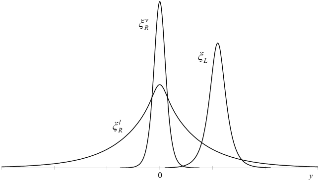
Figure 1: Schematic depiction of left-right overlaps for neutrino and charged lepton in the extra dimension: $\xi^{\nu.l}_{R}$, zero-mode wave function for right-handed neutrino and charged lepton; $\xi_{L}$, zero-mode wave function for left-handed leptonic doublet.

The localization and symmetry breakings along the extra dimension involve Yukawa couplings, e.g., in the form $f\bar{\Psi}_{1}\Phi\Psi_{1}+f\bar{\Psi}_{2}\Phi\Psi_{2}$, where $\Psi_{1}$ and $\Psi_{2}$ couple to the same scalar field with the same coupling constant to localize at the same point or shift position with the same amount. This suggests an $\mathrm{SU}(2)_{G}$ global symmetry among $\Psi_{1}$ and $\Psi_{2}$ in the extra-dimensional Yukawa sector. For the Yukawa sector in the extra dimension, therefore, the symmetry group of the theory can be written as the product of global and gauge groups, $G=G_{\text{gauge}}\otimes G_{\text{global}}$. Although the $\mathrm{SU}(2)_{G}$ global symmetry is limited to the extra-dimensional Yukawa sector, there is an analogous, however implicit, global $\mathrm{SU}(2)$ symmetry among $\Psi_{1}$ and $\Psi_{2}$ if only the strong $\mathrm{SU}(4)_{\mathrm{PS}}$ quartets are looked at, i.e., weak group neglected. The fact that the weak group representations of $\Psi_{1}$ and $\Psi_{2}$ differ means that such extensive symmetry is explicitly broken by $G_{W}$.

The fermion representation of the model for couplings with scalar fields in the extra dimension can be written as

$$\Psi\left({x^{\mu},y}\right)=\left({\begin{array}[]{*{20}c}{\begin{array}[]{*{20}c}{4,3,\bar{3}}\\ {4,\bar{3},3}\\ \end{array}}&;&2\\ \end{array}}\right)=\left({\begin{array}[]{*{20}c}{\Psi_{1}\left({x^{\mu},y}\right)}\\ {\Psi_{2}\left({x^{\mu},y}\right)}\\ \end{array}}\right),$$ (18)

where we used the notation $\left({\begin{array}[]{*{20}c}{\mathrm{Gauge}}&;&{\mathrm{Global}}\\ \end{array}}\right)$ to articulate the multiplet structure of $\Psi$ with respect to the gauge and global groups.

To find out the appropriate group representations of the background scalar fields, needed for localization and symmetry breakings, we should examine the bilinear form of $\Psi$ under $\mathrm{SU}(4)_{\mathrm{PS}}\otimes\mathrm{SU}(3)_{L}\otimes\mathrm{SU}(3)_{H}\otimes\mathrm{SU}(2)_{G}$, explicitly

$$\bar{\Psi}\left({x,y}\right)\Psi\left({x,y}\right)=\left({\begin{array}[]{*{20}c}{15\oplus 1,8\oplus 1,8\oplus 1}&;&{3\oplus 1}\\ \end{array}}\right).$$ (19)

From Eq. (19), one can pick suitable scalar fields to

1. Localize the right-handed and left-handed fermions in the extra dimension at different locations,

2. Give different profiles to up and down sectors of the right-handed fermions,

3. Differentiate between normal and unconventional fermions, also quarks and leptons.

In the following sections, we shall carry out these tasks one by one.

IV.1 Localization of fermions

To localize the SM-type fermions as chiral zero modes, we first note that we wrote the fermion representations of $\mathrm{PUT}_{2}$ as left-handed multiplets (see section III). Therefore, by choosing a chiral ${{\mathrm{S}_{1}}\mathord{\left/{\vphantom{{S_{1}}{\mathbb{Z}_{2}}}}\right.\kern-1.2pt}{\mathbb{Z}_{2}}}$ orbifold and positive couplings in the localization process Georgi et al. (2001), we can assign zero modes to all left-handed fields of the representation including the right handed fields which are written as charge conjugates. This way, the relevant 5D Dirac spinors transform as left-handed SM fermions. Symbolically, the 5D representation of the model as chiral zero mode can be imagined as

$$\Psi_{L}\left({x,y}\right)=\left({\begin{array}[]{*{20}c}{\Psi_{1L}\left(x\right)\xi_{1}\left(y\right)}\\ {\Psi_{2L}\left(x\right)\xi_{2}\left(y\right)}\\ \end{array}}\right),$$ (20)

where $\xi$’s take on the appropriate zero-mode wave functions for each constituent field of the multiplet. Throughout this work and for clarity, we denote the zero-mode wave functions of the left- and right-handed fields with subscripts $L$ and $R$, respectively.

For localization, consider a singlet scalar field $\Phi_{S}=\left({\begin{array}[]{*{20}c}{1,1,1}&;&1\\ \end{array}}\right)$. The gauge- and global-invariant Yukawa coupling of such scalar field with fermions looks like

$$\mathcal{L}_{S}=f_{S}\bar{\Psi}\Phi_{S}\Psi=f_{S}\left({\bar{\Psi}_{1}\Phi_{S}\Psi_{1}+\bar{\Psi}_{2}\Phi_{S}\Psi_{2}}\right),$$ (21)

where $f_{S}>0$. To localize at some non-zero point, $y\neq 0$, let the kink solution of $\Phi_{S}$ be in the form

$$\left\langle{\Phi_{S}}\right\rangle=h_{S}\left(y\right)+v_{S}\,.$$ (22)

The equation of motion for the zero-mode wave functions of the left- and right-handed SM-type fermions is then given by

$$\partial_{y}\xi_{L,R}+\left[{f_{S}h_{S}\left(y\right)+f_{S}v_{S}}\right]\xi_{L,R}=0\,.$$ (23)

However, if one wants to have left-right overlaps between the zero modes, one needs to separate the zero-mode wave functions of the left- and right-handed fields along the extra dimension. This can be done by moving the left- and right- handed zero-modes asymmetrically. To do this, we need to couple fermions to a background scalar field that would only acquire a minimum energy solution and not a kink solution. We introduce a scalar field $\Phi_{O}=\left({\begin{array}[]{*{20}c}{1,8,1}&;&1\\ \end{array}}\right)$, whose coupling with fermions takes the form

$$\mathcal{L}_{O}=-f_{O}\bar{\Psi}\Phi_{O}\Psi=-f_{O}\left(\bar{\Psi}_{1}\Phi_{O}\Psi_{1}+\bar{\Psi}_{2}\Phi_{O}\Psi_{2}\right),$$ (24)

where $f_{O}>0$. The minimum energy solution of $\Phi_{O}$ (which leaves $\mathrm{SU}(2)_{L}$ unbroken) for such asymmetrical shift can simply take on the eighth direction of $\mathrm{SU}(3)_{L}$, i.e.,

$$\left\langle{\Phi_{O}}\right\rangle=\delta\left({\begin{array}[]{*{20}c}1&0&0\\ 0&1&0\\ 0&0&{-2}\\ \end{array}}\right),$$ (25)

where $\delta$ is the vacuum expectation value (VEV) of $\Phi_{O}$. The coupling in Eq. (24), when $\Phi_{O}$ develops VEV, shifts the position of the left- and right-handed zero modes along the extra dimension differently, which is obvious from their equations of motion

$$\partial_{y}\xi_{L}\left(y\right)+\left[{f_{S}h_{S}\left(y\right)+f_{S}v_{S}-f_{O}\delta}\right]\xi_{L}\left(y\right)=0,$$ (26a)

$$\partial_{y}\xi_{R}\left(y\right)+\left[{f_{S}h_{S}\left(y\right)+f_{S}v_{S}+2f_{O}\delta}\right]\xi_{R}\left(y\right)=0.$$ (26b)

with $\delta\neq 0$. The possibility of $\delta=0$ will be discussed later. We remind ourselves that the left-handed zero-mode wave functions $\xi_{L}$, are $\mathrm{SU}(2)_{L}$ doublets, while the right-handed zero-mode wave functions $\xi_{R}$, are just singlets.

IV.2 Distinguishing the up and down sectors of the right-handed fermions

Since one sector of the right-handed SM-type fields are in $\Psi_{1}$ and the other in $\Psi_{2}$, distinguishing these two sectors along the extra dimension demands a coupling which differentiates between them in the extra dimension. Looking at Eq. (19), we consider two $\mathrm{SU}(2)_{G}$ triplet fields $\Phi_{T}=\left({\begin{array}[]{*{20}c}{1,1,1}&;&3\\ \end{array}}\right)$ and $\Phi^{\prime}_{T}=\left({\begin{array}[]{*{20}c}{1,8,1}&;&3\\ \end{array}}\right)$, for an asymmetrical profile changing. The Yukawa couplings with fermions would be

$$\mathcal{L}_{T}=f_{T}\bar{\Psi}\Phi_{T}\Psi+f^{\prime}_{T}\bar{\Psi}\Phi^{\prime}_{T}\Psi,$$ (27)

where $f_{T},f^{\prime}_{T}>0$. To alter the shapes of the right-handed zero-mode wave functions, these two triplet fields must attain kink solutions, they are

$$\left\langle{\Phi_{T}}\right\rangle=h_{T}\left(y\right)\left({\begin{array}[]{*{20}c}1&0\\ 0&{-1}\\ \end{array}}\right),$$ (28)

and

$$\left\langle{\Phi^{\prime}_{T}}\right\rangle=h^{\prime}_{T}\left(y\right)\left({\begin{array}[]{*{20}c}1&0&0\\ 0&1&0\\ 0&0&{-2}\\ \end{array}}\right)\otimes\left({\begin{array}[]{*{20}c}1&0\\ 0&{-1}\\ \end{array}}\right),$$ (29)

where $h_{T}\left(y\right)$ and $h^{\prime}_{T}\left(y\right)$ are the kink solutions of $\Phi_{T}$ and $\Phi^{\prime}_{T}$, respectively. The equations of motion for the zero-mode wave functions now read

$$\partial_{y}\xi_{L}\left(y\right)+\left[{f_{S}h_{S}\left(y\right)+f_{T}h_{T}\left(y\right)+f^{\prime}_{T}h^{\prime}_{T}\left(y\right)+f_{S}v_{S}-f_{O}\delta}\right]\xi_{L}\left(y\right)=0\,,$$ (30a)

$$\partial_{y}\xi_{R}^{up}\left(y\right)+\left[{f_{S}h_{S}\left(y\right)+\left({f_{T}h_{T}\left(y\right)-2f^{\prime}_{T}h^{\prime}_{T}\left(y\right)}\right)+f_{S}v_{S}-2f_{O}\delta}\right]\xi_{R}^{up}\left(y\right)=0\,,$$ (30b)

$$\partial_{y}\xi_{R}^{up}\left(y\right)+\left[{f_{S}h_{S}\left(y\right)-\left({f_{T}h_{T}\left(y\right)-2f^{\prime}_{T}h^{\prime}_{T}\left(y\right)}\right)+f_{S}v_{S}-2f_{O}\delta}\right]\xi_{R}^{up}\left(y\right)=0\,,$$ (30c)

where $\xi_{R}^{up}$ and $\xi_{R}^{down}$ refer to the right-handed zero-mode wave functions of $\Psi_{1}$ (i.e., those of $d$, $D$, $l_{d}$, and $\nu$) and $\Psi_{2}$ (i.e., those of $u$, $U$, $l_{u}$, and $l$), respectively. The doublet $\xi_{L}$ still refers to both normal and unconventional left-handed fermion zero-mode wave functions, which means the left-handed fermions of $\Psi_{1}$.

It can be seen, from Eqs. (30b and 30c) that the profiles of the right-handed zero-mode wave functions of $\Psi_{1}$ and $\Psi_{2}$, which we denote by $\xi_{R}^{up}$ and $\xi_{R}^{down}$, are now different: a broad wave function for $\xi_{R}^{down}$ and a narrow wave function for $\xi_{R}^{up}$. This disparity between the profiles of the two sectors of right-handed zero modes may become more clear in section IV.5. Let us define

$$h_{sym}\left(y\right)\equiv f_{S}h_{S}\left(y\right)+\left({f_{T}h_{T}\left(y\right)-2f^{\prime}_{T}h^{\prime}_{T}\left(y\right)}\right)\,,$$ (31a)

$$h_{asym}\left(y\right)\equiv f_{S}h_{S}\left(y\right)-\left({f_{T}h_{T}\left(y\right)-2f^{\prime}_{T}h^{\prime}_{T}\left(y\right)}\right)\,,$$ (31b)

for future compactness of equations.

IV.3 Distinguishing normal and unconventional fermions, quarks and leptons

As the geometry of the zero-mode wave functions in the extra dimension determines the overlaps and therefore the effective Yukawa couplings, one would like to differentiate between the zero-mode wave functions of normal and unconventional fermions, also between those of quarks and leptons. Since these fermions are mixed by groups $\mathrm{SU}(4)_{\mathrm{PS}}$ and $\mathrm{SU}(3)_{H}$, breaking those symmetries along the extra dimension seems plausible. The desired symmetry breaking can be achieved by four scalar fields, which only develop VEV’s and not kink solutions. The scalar fields are $\Sigma=\left({\begin{array}[]{*{20}c}{15,8,1}&;&1\\ \end{array}}\right)$, $\Sigma^{\prime}=\left({\begin{array}[]{*{20}c}{15,1,1}&;&1\\ \end{array}}\right)$, $\Omega=\left({\begin{array}[]{*{20}c}{15,8,8}&;&1\\ \end{array}}\right)$, and $\Omega^{\prime}=\left({\begin{array}[]{*{20}c}{15,1,8}&;&1\\ \end{array}}\right)$, with Yukawa couplings in the form

$$\mathcal{L}_{Y}=\bar{\Psi}\left({f_{\Sigma}\Sigma+f_{\Sigma^{\prime}}\Sigma^{\prime}+f_{\Omega}\Omega+f_{\Omega^{\prime}}\Omega^{\prime}}\right)\Psi,$$ (32)

where $f_{\Sigma},\,f_{\Sigma^{\prime}},\,f_{\Omega},\,f_{\Omega^{\prime}}>0$. The minimum energy solutions of these fields are taken as

$$\left\langle{\Sigma}\right\rangle=\sigma\left({\begin{array}[]{*{20}c}1&0&0&0\\ 0&1&0&0\\ 0&0&1&0\\ 0&0&0&{-3}\\ \end{array}}\right)\otimes\left({\begin{array}[]{*{20}c}1&0&0\\ 0&1&0\\ 0&0&{-2}\\ \end{array}}\right),$$ (33a)

$$\left\langle{\Sigma^{\prime}}\right\rangle=\sigma^{\prime}\left({\begin{array}[]{*{20}c}1&0&0&0\\ 0&1&0&0\\ 0&0&1&0\\ 0&0&0&{-3}\\ \end{array}}\right),$$ (33b)

$$\left\langle{\Omega}\right\rangle=\left({\begin{array}[]{*{20}c}1&0&0&0\\ 0&1&0&0\\ 0&0&1&0\\ 0&0&0&{-3}\\ \end{array}}\right)\otimes\left({\begin{array}[]{*{20}c}1&0&0\\ 0&1&0\\ 0&0&{-2}\\ \end{array}}\right)\otimes\left({\begin{array}[]{*{20}c}{\omega}&0&0\\ 0&{-\omega}&0\\ 0&0&0\\ \end{array}}\right),$$ (33c)

$$\left\langle{\Omega^{\prime}}\right\rangle=\left({\begin{array}[]{*{20}c}1&0&0&0\\ 0&1&0&0\\ 0&0&1&0\\ 0&0&0&{-3}\\ \end{array}}\right)\otimes\left({\begin{array}[]{*{20}c}{\omega^{\prime}}&0&0\\ 0&{-\omega^{\prime}}&0\\ 0&0&0\\ \end{array}}\right).$$ (33d)

Similar to $\Phi_{O}$’s role in section IV.1, the role of these scalar fields is to shift the positions of the zero-mode wave functions of normal and unconventional fermions, even those of quarks and leptons along the extra dimension. That means different left-right separations for each one of those classes, which would indicate different overlaps and therefore effective Yukawa couplings.

Let us start with the left-handed zero-mode wave functions. Their equation of motion, Eq. (30a), now splits into four different equations

$$\partial_{y}\xi_{L}^{q}\left(y\right)+\left[{f_{S}h_{S}\left(y\right)+f_{T}h_{T}\left(y\right)+f^{\prime}_{T}h^{\prime}_{T}\left(y\right)+f_{S}v_{S}-f_{O}\delta+X_{L}^{q}}\right]\xi_{L}^{q}\left(y\right)=0\,,$$ (34a)

$$\partial_{y}\xi_{L}^{Q}\left(y\right)+\left[{f_{S}h_{S}\left(y\right)+f_{T}h_{T}\left(y\right)+f^{\prime}_{T}h^{\prime}_{T}\left(y\right)+f_{S}v_{S}-f_{O}\delta+X_{L}^{Q}}\right]\xi_{L}^{Q}\left(y\right)=0\,,$$ (34b)

$$\partial_{y}\xi_{L}^{l}\left(y\right)+\left[{f_{S}h_{S}\left(y\right)+f_{T}h_{T}\left(y\right)+f^{\prime}_{T}h^{\prime}_{T}\left(y\right)+f_{S}v_{S}-f_{O}\delta-3X_{L}^{q}}\right]\xi_{L}^{l}\left(y\right)=0\,,$$ (34c)

$$\partial_{y}\xi_{L}^{L}\left(y\right)+\left[{f_{S}h_{S}\left(y\right)+f_{T}h_{T}\left(y\right)+f^{\prime}_{T}h^{\prime}_{T}\left(y\right)+f_{S}v_{S}-f_{O}\delta-3X_{L}^{Q}}\right]\xi_{L}^{L}\left(y\right)=0\,,$$ (34d)

where

$$X_{L}^{q}=f_{\Sigma}\sigma+f_{\Sigma^{\prime}}\sigma^{\prime}+f_{\Omega}\omega+f_{\Omega^{\prime}}\omega^{\prime}\,,$$ (35a)

$$X_{L}^{Q}=f_{\Sigma}\sigma+f_{\Sigma^{\prime}}\sigma^{\prime}-f_{\Omega}\omega-f_{\Omega^{\prime}}\omega^{\prime}\,,$$ (35b)

In Eqs. (34), the superscripts $q$, $l$, $Q$, and $L$, correspond to normal quark, normal lepton, unconventional quark and unconventional lepton, respectively.

The two equations of motion for right-handed zero-mode wave functions, Eqs. (30b and 30c), also split into eight equations for those of quarks and leptons, unconventional and normal. For $\xi_{R}^{up}$, we obtain

$$\partial_{y}\xi_{R}^{q,up}\left(y\right)+\left[{h_{sym}\left(y\right)+f_{S}v_{S}+2f_{O}\delta+X_{R}^{q}}\right]\xi_{R}^{q}\left(y\right)=0\,,$$ (36a)

$$\partial_{y}\xi_{R}^{Q,up}\left(y\right)+\left[{h_{sym}\left(y\right)+f_{S}v_{S}+2f_{O}\delta+X_{R}^{Q}}\right]\xi_{R}^{Q}\left(y\right)=0\,,$$ (36b)

$$\partial_{y}\xi_{R}^{l,up}\left(y\right)+\left[{h_{sym}\left(y\right)+f_{S}v_{S}+2f_{O}\delta-3X_{R}^{q}}\right]\xi_{R}^{l}\left(y\right)=0\,,$$ (36c)

$$\partial_{y}\xi_{R}^{L,up}\left(y\right)+\left[{h_{sym}\left(y\right)+f_{S}v_{S}+2f_{O}\delta-3X_{R}^{Q}}\right]\xi_{R}^{L}\left(y\right)=0\,,$$ (36d)

where

$$X_{R}^{q}=-2f_{\Sigma}\sigma+f_{\Sigma^{\prime}}\sigma^{\prime}-2f_{\Omega}\omega+f_{\Omega^{\prime}}\omega^{\prime}\,,$$ (37a)

$$X_{R}^{Q}=-2f_{\Sigma}\sigma+f_{\Sigma^{\prime}}\sigma^{\prime}+2f_{\Omega}\omega-f_{\Omega^{\prime}}\omega^{\prime}\,,$$ (37b)

while for $\xi_{R}^{down}$ the same equations are valid with $h_{sym}\left(y\right)\rightarrow h_{asym}\left(y\right)$ of Eqs. (31). From Eqs. (34 and 36), it is clear that due to strong and horizontal symmetry breaking, each type of left- and right-handed zero mode is localized at different point in the extra dimension. Therefore, the left-right separations which determine the overlaps would be different for each type, as we desired. Although Eqs. (34 and 36) seem to suggest that the displacements due to strong and horizontal symmetry breakings are expressed in terms of four parameters $X_{L}^{q}$, $X_{L}^{Q}$, $X_{R}^{q}$, and $X_{R}^{Q}$, there are only two independent parameters involved. For example, since

$$X_{L}^{q}+X_{L}^{Q}=2f_{\Sigma}\sigma+2f_{\Sigma^{\prime}}\sigma^{\prime}\,,$$ (38a)

$$X_{R}^{q}+X_{R}^{Q}=-4f_{\Sigma}\sigma+2f_{\Sigma^{\prime}}\sigma^{\prime}\,,$$ (38b)

once one fixes the two coupling constants and vacua on the right hand side of Eqs. (38), the $X$’s can be expressed in terms of each other. That means two of these $X$’s are indeed arbitrary and can be viewed as references for the other two.

Hence, let us set $X_{R}^{q}=X_{R}^{Q}=0$ and let $X_{L}^{q}$, $X_{L}^{Q}$ be the two independent parameters of strong and horizontal symmetry breakings, they become

$$X_{L}^{q}=3f_{\Sigma}\sigma+3f_{\Omega}\omega\,,$$ (39a)

$$X_{L}^{Q}=3f_{\Sigma}\sigma-3f_{\Omega}\omega\,.$$ (39b)

At this stage and to differentiate the normal fermions from the unconventional ones, we demand the important phenomenological constraint

$$f_{\Sigma}\sigma=f_{\Omega}\omega\,.$$ (40)

This assumption separates the zero-mode wave functions of normal and unconventional SM-type fermions in a fashion that results in stronger left-right overlaps for unconventional fermions and consequently higher mass scales. That is what we expect, since the unconventional fermions have not been experimentally detected yet. With the constraint of Eq. (40), the two independent distances $X_{L}^{q}$ and $X_{L}^{Q}$ become

$$X_{L}^{q}=6f_{\Omega}\omega\,,$$ (41a)

$$X_{L}^{Q}=0\,,$$ (41b)

Therefore, the zero-mode wave functions of left-handed SM-type fermions satisfy

$$\partial_{y}\xi_{L}^{q}\left(y\right)+\left[{f_{S}h_{S}\left(y\right)+f_{T}h_{T}\left(y\right)+f^{\prime}_{T}h^{\prime}_{T}\left(y\right)+f_{S}v_{S}-f_{O}\delta+6f_{\Omega}\omega}\right]\xi_{L}^{q}\left(y\right)=0\,,$$ (42a)

$$\partial_{y}\xi_{L}^{Q}\left(y\right)+\left[{f_{S}h_{S}\left(y\right)+f_{T}h_{T}\left(y\right)+f^{\prime}_{T}h^{\prime}_{T}\left(y\right)+f_{S}v_{S}-f_{O}\delta}\right]\xi_{L}^{Q}\left(y\right)=0\,,$$ (42b)

$$\partial_{y}\xi_{L}^{l}\left(y\right)+\left[{f_{S}h_{S}\left(y\right)+f_{T}h_{T}\left(y\right)+f^{\prime}_{T}h^{\prime}_{T}\left(y\right)+f_{S}v_{S}-f_{O}\delta-18f_{\Omega}\omega}\right]\xi_{L}^{l}\left(y\right)=0\,,$$ (42c)

$$\partial_{y}\xi_{L}^{L}\left(y\right)+\left[{f_{S}h_{S}\left(y\right)+f_{T}h_{T}\left(y\right)+f^{\prime}_{T}h^{\prime}_{T}\left(y\right)+f_{S}v_{S}-f_{O}\delta}\right]\xi_{L}^{L}\left(y\right)=0\,,$$ (42d)

Looking at Eqs. (42b and 42d), one notices that $\xi_{L}^{Q}=\xi_{L}^{L}$. On the other hand, the zero-mode wave functions for the right-handed SM-type fermions still obey Eqs. (30b and 30c).

IV.4 Simplification of numerical algorithm

So far, we have localized SM-type fermions at different points and given different shapes to the right-handed zero mode wave functions by symmetry breakings along the extra dimension. The equations of motion for left- and right-handed zero mode wave functions can be simplified considerably, for numerical ease, however without affecting the values of left-right overlaps. To begin with, let us assume

$$f_{S}v_{S}=-2f_{O}\delta\,,$$ (43)

which preserves the distance between the left- and right-handed zero modes, however places the right-handed zero modes at the origin. As the distance and profiles of the zero modes are the only important factors in determining the overlaps, such assumption only simplifies numerical procedure.

On the other hand, in analogy with the idea presented in Refs. Hung (2003, 2005), where the difference in profiles for the up and down sectors of the right-handed zero-mode wave functions is sufficient to describe the sizes of corresponding overlaps, we may also consider

$$f^{\prime}_{T}h^{\prime}_{T}\left(y\right)=-f_{T}h_{T}\left(y\right)\,,$$ (44)

which simplifies the left-handed zero-mode wave functions. The dissimilar (narrow and broad) profiles of the right-handed zero-mode wave functions $\xi_{R}^{up}$ and $\xi_{R}^{down}$ remain in place regardless of the condition of Eq. (44) and since that difference in shapes is what matters (see Fig. 1), the numerical value of left-right overlaps will not change. With these simplifications, the equations of motion for zero-mode wave functions read

$$\partial_{y}\xi_{L}^{q}\left(y\right)+\left[{f_{S}h_{S}\left(y\right)-3f_{O}\delta+6f_{\Omega}\omega}\right]\xi_{L}^{q}\left(y\right)=0\,,$$ (45a)

$$\partial_{y}\xi_{L}^{Q}\left(y\right)+\left[{f_{S}h_{S}\left(y\right)-3f_{O}\delta}\right]\xi_{L}^{Q}\left(y\right)=0\,,$$ (45b)

$$\partial_{y}\xi_{L}^{l}\left(y\right)+\left[{f_{S}h_{S}\left(y\right)-3f_{O}\delta-18f_{\Omega}\omega}\right]\xi_{L}^{l}\left(y\right)=0\,,$$ (45c)

$$\partial_{y}\xi_{L}^{L}\left(y\right)+\left[{f_{S}h_{S}\left(y\right)-3f_{O}\delta}\right]\xi_{L}^{L}\left(y\right)=0\,,$$ (45d)

and

$$\partial_{y}\xi_{R}^{up}\left(y\right)+\left[{f_{S}h_{S}\left(y\right)+3f_{T}h_{T}\left(y\right)}\right]\xi_{R}^{up}\left(y\right)=0\,,$$ (46a)

$$\partial_{y}\xi_{R}^{down}\left(y\right)+\left[{f_{S}h_{S}\left(y\right)-3f_{T}h_{T}\left(y\right)}\right]\xi_{R}^{down}\left(y\right)=0\,.$$ (46b)

In mass scale calculations, we find out that the distances between localized left-handed and right-handed zero-mode wave functions along the extra dimension are needed. Estimating those separations is the subject of the next section.

IV.5 Left-right separations along the extra dimension

The localization process of SM-type fermions involved scalar fields, with classical kink solutions. The kink solutions, however, yet to be specified. In order to estimate the left-right separations, we give a Gaussian shape to zero mode wave functions. Let us consider a linear approximation for the kink solutions, explicitly

$$h_{S}\left(y\right)\approx\mu_{S}^{2}y\,,$$ (47a)

$$h_{T}\left(y\right)\approx\mu_{T}^{2}y\,.$$ (47b)

In this linear approximation, the equations of motion for the right-handed zero-mode wave functions, Eqs. (46), become

$$\partial_{y}\xi_{R}^{up}\left(y\right)+\left({f_{S}\mu_{S}^{2}+3f_{T}\mu_{T}^{2}}\right)y\xi_{R}^{up}\left(y\right)=0\,,$$ (48a)

$$\partial_{y}\xi_{R}^{down}\left(y\right)+\left({f_{S}\mu_{S}^{2}-3f_{T}\mu_{T}^{2}}\right)y\xi_{R}^{down}\left(y\right)=0\,,$$ (48b)

The Gaussians defined by Eqs. (48) are clearly localized at $y=0$, meaning

$$y_{R}^{up}=y_{R}^{down}=0\,,$$ (49)

where $y_{R}^{up}$ corresponds to the location of the right-handed zero modes of $\Psi_{1}$ (i.e., those of $d$, $D$, $l_{d}$, and $\nu$) and $y_{R}^{down}$ refers to the location of the right-handed zero modes of $\Psi_{2}$ (i.e., those of $u$, $U$, $l_{u}$, and $l$). From Eqs. (48), one clearly sees the shape notion of narrow $\xi_{R}^{up}$ and wide $\xi_{R}^{down}$. The locations of the left-handed zero-mode wave functions, on the other hand, can be determined from their differential equations, Eqs. (45). Those equations, in the linear approximation scheme, now read

$$\partial_{y}\xi_{L}^{q}\left(y\right)+\left({f_{S}\mu_{S}^{2}y-3f_{O}\delta+6f_{\Omega}\omega}\right)\xi_{L}^{q}\left(y\right)=0\,,$$ (50a)

$$\partial_{y}\xi_{L}^{Q}\left(y\right)+\left({f_{S}\mu_{S}^{2}y-3f_{O}\delta}\right)\xi_{L}^{Q}\left(y\right)=0\,,$$ (50b)

$$\partial_{y}\xi_{L}^{l}\left(y\right)+\left({f_{S}\mu_{S}^{2}y-3f_{O}\delta-18f_{\Omega}\omega}\right)\xi_{L}^{l}\left(y\right)=0\,,$$ (50c)

$$\partial_{y}\xi_{L}^{L}\left(y\right)+\left({f_{S}\mu_{S}^{2}y-3f_{O}\delta}\right)\xi_{L}^{L}\left(y\right)=0\,.$$ (50d)

For our future convenience, let us define

$$w\equiv\frac{3f_{O}\delta}{f_{\Omega}\omega}\,.$$ (51)

With this definition, The locations of localized left-handed zero-mode wave functions can be written as

$$y_{L}^{q} =\frac{f_{\Omega}\omega}{f_{S}\mu_{S}^{2}}\left({w-6}\right)\,,$$ (52a)

$$y_{L}^{Q} =\frac{f_{\Omega}\omega}{f_{S}\mu_{S}^{2}}w\,,$$ (52b)

$$y_{L}^{l} =\frac{f_{\Omega}\omega}{f_{S}\mu_{S}^{2}}\left({w+18}\right)\,,$$ (52c)

$$y_{L}^{L} =\frac{f_{\Omega}\omega}{f_{S}\mu_{S}^{2}}w\,.$$ (52d)

The superscripts on $y$’s in Eqs. (52) have the same meanings explained in sections IV.2 and IV.3 for $\xi$’s. Each location given in Eqs. (52) is applicable to both components of the left-handed zero-mode wave function doublet to which it refers. Since the mass terms involve left- and right-handed fields, the relevant wave function separations are those between the left- and right-handed ones. Using the locations we already found, those left-right separations can be computed easily. They are

• For normal quarks

  $$\left|{\Delta y^{q}}\right|=\left|{y_{R}-y_{L}^{q}}\right|=\left|{\frac{f_{\Omega}\omega}{f_{S}\mu_{S}^{2}}\left({6-w}\right)}\right|,$$ (53)

• For normal leptons

  $$\left|{\Delta y^{l}}\right|=\left|{y_{R}-y_{L}^{l}}\right|=\left|{\frac{f_{\Omega}\omega}{f_{S}\mu_{S}^{2}}\left({w+18}\right)}\right|,$$ (54)

• For unconventional quarks and leptons

  $$\left|{\Delta y^{L}}\right|=\left|{\Delta y^{Q}}\right|=\left|{y_{R}-y_{L}^{L}}\right|=\left|{y_{R}-y_{L}^{Q}}\right|=\left|{\frac{f_{\Omega}\omega}{f_{S}\mu_{S}^{2}}w}\right|.$$ (55)

In these left-right separations, $\Delta y$’s refer to both up and down sectors of each flavor doublet and $y_{R}=y_{R}^{up}=y_{R}^{down}$. The identical left-right separations of unconventional quarks and leptons, Eq. (55), imply similar mass scales. Obviously, the magnitude of such mass scale can be large and remains to be explored. Alternatively, and with the help of Eqs. (53 and 54), the relation between the wave function separations of quarks and leptons can be found, i.e.,

$$\left|{\Delta y^{l}}\right|=3\left|{\frac{{{w\mathord{\left/{\vphantom{w{18}}}\right.\kern-1.2pt}{18}}+1}}{{1-{w\mathord{\left/{\vphantom{w6}}\right.\kern-1.2pt}6}}}}\right|\left|{\Delta y^{q}}\right|$$ (56)

We can also find relationship between the left-right separations of unconventional fermions and ordinary quarks, i.e.,

$$\left|{\Delta y^{Q/L}}\right|=\left|{\frac{w}{6-w}}\right|\left|{\Delta y^{q}}\right|=\frac{1}{4}\left({\frac{\left|{\Delta y^{l}}\right|}{\left|{\Delta y^{q}}\right|}-3}\right)\left|{\Delta y^{q}}\right|.$$ (57)

Since the left-right separations are determinant factors in mass scale computations, Eq. (56) implies relationship between the mass scales of ordinary quarks and leptons in one generation, as fixing one would restrain the other.

This can also be extended to unconventional fermions, as Eq. (57) relates the left-right separations of unconventional fermions to those of ordinary fermions. Thus the masses of unconventional fermions cannot just be heavy enough to escape detection; they must yield meaningful masses for ordinary fermions, as the known physics is concerned.

We have then arrived at a point where the masses of unconventional fermions not only should comply with the existent experimental check on ordinary quarks and charged lepton’s masses but they could in principle restrain the mass scales for the neutrino sector of ordinary leptons, as their left-right separations in the extra dimension restrain the left-right separations of ordinary leptons including those of neutrinos.

Let us now discuss the possibility of having $\delta=0$, which we left aside in section IV.1. Obviously, $\delta=0$ corresponds to $w=0$, which would mean $\left|{\Delta y^{l}}\right|=3\left|{\Delta y^{q}}\right|$ and $\left|{\Delta y^{Q/L}}\right|=0$. Phenomenologically, we prefer $\delta\neq 0$ for the reason that will be clear when we give numerical results for the mass scales. With a minimum at $w=0$, Eq. (56) can be also written as $\left|{\Delta y^{l}}\right|\geq 3\left|{\Delta y^{q}}\right|$, which clearly indicates that lepton’s wave function overlaps can be potentially weaker than those of quarks. This seems plausible knowing the profound differences between the mass scales of quarks and leptons.

V Return to four dimensions: The mass scales

Speaking of SM-type fermion mass terms and mass scales implies that the gauge symmetry is reduced to that of the SM and is going to break further down by the SM Higgs vacuum. A complete analysis of the gauge symmetry breakdown of the model is rather lengthy and is not consistent with the flow of the paper at this point. However, the necessary scalar fields for the gauge symmetry breakdown and the mixing of charged gauge bosons are crucial to our analyses in sections VI and VII. For that reason and completeness, a detailed gauge symmetry breakdown is given in Appendix A.

As we only concentrate on the mass scales, we therefore will not discuss issues such as the fermion mixings in the mass matrix Dienes and Hossenfelder (2006). We follow the mass scale calculations with some rough numerical analysis.

V.1 Effective Yukawa couplings and the mass scales

Dirac mass terms for chiral fermions involve couplings of left-handed and right-handed fields with a Higgs field, which acquires VEV and breaks the SM symmetry as well. The minimal SM symmetry breakdown of our model can occur through a Higgs multiplet transforming as $\Theta=\left(1,8,8\right)$. The decomposition of $\Theta$’s $\mathrm{SU}(3)_{L}$ octet in terms of $\mathrm{SU}(2)_{L}\otimes\mathrm{U}(1)_{Y}$ multiplets or quantum numbers

$$\left[8\right]_{\mathrm{SU}\left(3\right)_{L}}=\left(3,0\right)\oplus\left(2,1\right)\oplus\left(2,-1\right)\oplus\left(1,0\right),$$ (58)

shows that $\Theta$ indeed possesses a SM Higgs field, which we denote by $H=\left({2,1}\right)$. Thus, $\Theta$ can break the SM symmetry and give mass to chiral fermions by developing a VEV in $H$. The Yukawa couplings between the left- and right-handed SM-type fermions can be written in the form

$$\mathcal{L}_{\mathrm{mass}}=\kappa_{1}\Psi_{1}^{T}\Theta C\Psi_{2}^{\ast}+\kappa_{2}\Psi_{1}^{T}\tilde{\Theta}C\Psi_{1}^{\ast}+h.c.\,.$$ (59)

In the above couplings, $\kappa_{1}$, $\kappa_{2}$ can be different in general, $\tilde{\Theta}=i\hat{\lambda}_{2L}\Theta^{*}$, and $C=i\gamma^{2}\gamma^{0}$. The mass terms in Eq. (59) seem compact but they can be expanded very easily. For example, they yield

$$\mathcal{L}_{\mathrm{mass}}^{q}=\kappa_{1}\frac{v}{{\sqrt{2}}}\bar{u}_{L}u_{R}-\kappa_{2}\frac{v}{{\sqrt{2}}}\bar{d}_{L}d_{R}+h.c.\;,$$ (60)

for normal quarks. These mass expressions have been worked out for transparency in Appendix A. Similar expressions for other SM-type fermions can be obtained easily.

We assume a delocalized Higgs field along the extra dimension and use its lowest KK mode, which entirely depends on 4D coordinates. This means that the zero mode of the Higgs field is independent of $y$, and can be written as, e.g., $H^{0}\left({x,y}\right)=K\phi\left(x\right)$. The zero mode of the SM Higgs field $\phi$, then obtains VEV in the usual form $\bigl{(}\begin{smallmatrix}0\\ {{v\mathord{\left/{\vphantom{v{\sqrt{2}}}}\right.\kern-1.2pt}{\sqrt{2}}}}\end{smallmatrix}\bigl{)}$.

The mass terms involve Yukawa couplings determining the magnitude of each mass term. In our model and in four dimensional space, those couplings can be viewed as “effective” Yukawa couplings whose strengths are determined by the geometry of the zero-mode wave functions in the extra dimension. The reduction to 4D space is simply done by integrating the extra dimension out, and that is how the couplings in mass terms become “effective” 4D Yukawa couplings.

Mass scales can be computed from the mass terms in Eq. (59). To proceed, we define dimensionless couplings

$$g_{Y1,2}=\kappa_{1,2}K\,.$$ (61)

The relationship between the mass scales and the mass matrix is given by

$$\mathcal{M}=\Lambda M\,,$$ (62)

where $M$ is a dimensionless matrix, whose form depends on the model for fermion masses. In our case, we may write explicitly

$$\mathcal{M}_{u,d,\nu,l,U,D,l_{u},l_{d}}=\Lambda_{u,d,\nu,l,U,D,l_{u},l_{d}}M_{u,d,\nu,l,U,D,l_{u},l_{d}}\;,$$ (63)

where $\Lambda_{u,d,\nu,l,U,D,l_{u},l_{d}}$ are the mass scales of interest and the subscripts refer to the SM-type fermions of the theory. The mass scales in 4D space are proportional to the 4D effective Yukawa couplings, which in turn are proportional to the overlaps between the relevant left- and right-handed zero-mode wave functions in the extra dimension. Therefore, they simply are

$$\Lambda_{u} =\frac{v}{\sqrt{2}}g_{Y1}\int_{0}^{L}{dy\xi_{L}^{q}}\left(y\right)\xi_{R}^{down}\left(y\right)\qquad; \Lambda_{d} =\frac{v}{\sqrt{2}}g_{Y2}\int_{0}^{L}{dy\xi_{L}^{q}}\left(y\right)\xi_{R}^{up}\left(y\right),$$ (64)

$$\Lambda_{\nu} =\frac{v}{\sqrt{2}}g_{Y2}\int_{0}^{L}{dy\xi_{L}^{l}}\left(y\right)\xi_{R}^{up}\left(y\right)\qquad\;\;\;; \Lambda_{l} =\frac{v}{\sqrt{2}}g_{Y1}\int_{0}^{L}{dy\xi_{L}^{l}}\left(y\right)\xi_{R}^{down}\left(y\right),$$ (65)

$$\Lambda_{U} =\frac{v}{\sqrt{2}}g_{Y1}\int_{0}^{L}{dy\xi_{L}^{Q}}\left(y\right)\xi_{R}^{down}\left(y\right)\qquad; \Lambda_{D} =\frac{v}{\sqrt{2}}g_{Y2}\int_{0}^{L}{dy\xi_{L}^{Q}}\left(y\right)\xi_{R}^{up}\left(y\right),$$ (66)

$$\Lambda_{l_{u}} =\frac{v}{\sqrt{2}}g_{Y1}\int_{0}^{L}{dy\xi_{L}^{L}}\left(y\right)\xi_{R}^{down}\left(y\right)\qquad; \Lambda_{l_{d}} =\frac{v}{\sqrt{2}}g_{Y2}\int_{0}^{L}{dy\xi_{L}^{L}}\left(y\right)\xi_{R}^{up}\left(y\right).$$ (67)

Note that the left-handed $\xi_{L}$’s appearing in Eqs. (64) are no longer doublets, but the relevant components of those doublets. The fact is that the geometry of each flavor component is the same as that assigned to the corresponding doublet. As we are only concerned with the geometry of zero-mode wave functions, we do not introduce new notation for the flavor components, as if they were the relevant doublets. There are two possibilities that one can explore: $g_{Y1}=g_{Y2}$ and $g_{Y1}\neq g_{Y2}$. The relationships between the mass scales may depend on those choices.

1. $g_{Y1}=g_{Y2}$ : One can write all sorts of ratios, which would only depend on wave function overlaps. For example, we can write ratios relating mass scales of two sectors of one family, or ratios involving mass scales from different families. Some of those ratios are

   $$\frac{{\Lambda_{d}}}{{\Lambda_{u}}}=\frac{{\int_{0}^{L}{dy\xi_{L}^{q}}\left(y\right)\xi_{R}^{up}\left(y\right)}}{{\int_{0}^{L}{dy\xi_{L}^{q}}\left(y\right)\xi_{R}^{down}\left(y\right)}}\,,$$ (68a)

   $$\frac{{\Lambda_{\nu}}}{{\Lambda_{l}}}=\frac{{\int_{0}^{L}{dy\xi_{L}^{l}}\left(y\right)\xi_{R}^{up}\left(y\right)}}{{\int_{0}^{L}{dy\xi_{L}^{l}}\left(y\right)\xi_{R}^{down}\left(y\right)}}\,,$$ (68b)

   $$\frac{{\Lambda_{D}}}{{\Lambda_{U}}}=\frac{{\int_{0}^{L}{dy\xi_{L}^{Q}}\left(y\right)\xi_{R}^{up}\left(y\right)}}{{\int_{0}^{L}{dy\xi_{L}^{Q}}\left(y\right)\xi_{R}^{down}\left(y\right)}}\,,$$ (68c)

   $$\frac{{\Lambda_{\nu}}}{{\Lambda_{u}}}=\frac{{\int_{0}^{L}{dy\xi_{L}^{l}}\left(y\right)\xi_{R}^{up}\left(y\right)}}{{\int_{0}^{L}{dy\xi_{L}^{q}}\left(y\right)\xi_{R}^{down}\left(y\right)}}\,,$$ (68d)

   $$\frac{{\Lambda_{l}}}{{\Lambda_{u}}}=\frac{{\int_{0}^{L}{dy\xi_{L}^{l}}\left(y\right)\xi_{R}^{down}\left(y\right)}}{{\int_{0}^{L}{dy\xi_{L}^{q}}\left(y\right)\xi_{R}^{down}\left(y\right)}}\,,$$ (68e)

   $$\frac{{\Lambda_{D}}}{{\Lambda_{u}}}=\frac{{\int_{0}^{L}{dy\xi_{L}^{Q}}\left(y\right)\xi_{R}^{up}\left(y\right)}}{{\int_{0}^{L}{dy\xi_{L}^{q}}\left(y\right)\xi_{R}^{down}\left(y\right)}}\,,$$ (68f)

   $$\frac{{\Lambda_{U}}}{{\Lambda_{d}}}=\frac{{\int_{0}^{L}{dy\xi_{L}^{Q}}\left(y\right)\xi_{R}^{down}\left(y\right)}}{{\int_{0}^{L}{dy\xi_{L}^{q}}\left(y\right)\xi_{R}^{up}\left(y\right)}}\,,$$ (68g)

   $$\frac{{\Lambda_{\nu}}}{{\Lambda_{U}}}=\frac{{\int_{0}^{L}{dy\xi_{L}^{l}}\left(y\right)\xi_{R}^{up}\left(y\right)}}{{\int_{0}^{L}{dy\xi_{L}^{Q}}\left(y\right)\xi_{R}^{down}\left(y\right)}}\,,$$ (68h)

   $$\frac{{\Lambda_{l}}}{{\Lambda_{D}}}=\frac{{\int_{0}^{L}{dy\xi_{L}^{l}}\left(y\right)\xi_{R}^{down}\left(y\right)}}{{\int_{0}^{L}{dy\xi_{L}^{Q}}\left(y\right)\xi_{R}^{up}\left(y\right)}}\,.$$ (68i)

   One notices that the ratios involving unconventional leptons are identical to those of unconventional quarks, since they share the same left-handed wave functions and the same separations.

2. $g_{Y1}\neq g_{Y2}$: In this case, we may still find some ratios, depending only on wave function overlaps. They are

   $$\frac{{\Lambda_{l}}}{{\Lambda_{u}}}=\frac{{\int_{0}^{L}{dy\xi_{L}^{l}}\left(y\right)\xi_{R}^{down}\left(y\right)}}{{\int_{0}^{L}{dy\xi_{L}^{q}}\left(y\right)\xi_{R}^{down}\left(y\right)}}\,,$$ (69a)

   $$\frac{{\Lambda_{\nu}}}{{\Lambda_{d}}}=\frac{{\int_{0}^{L}{dy\xi_{L}^{l}}\left(y\right)\xi_{R}^{up}\left(y\right)}}{{\int_{0}^{L}{dy\xi_{L}^{q}}\left(y\right)\xi_{R}^{up}\left(y\right)}}\,,$$ (69b)

   $$\frac{{\Lambda_{U}}}{{\Lambda_{u}}}=\frac{{\int_{0}^{L}{dy\xi_{L}^{Q}}\left(y\right)\xi_{R}^{down}\left(y\right)}}{{\int_{0}^{L}{dy\xi_{L}^{q}}\left(y\right)\xi_{R}^{down}\left(y\right)}}\,,$$ (69c)

   $$\frac{{\Lambda_{D}}}{{\Lambda_{d}}}=\frac{{\int_{0}^{L}{dy\xi_{L}^{Q}}\left(y\right)\xi_{R}^{up}\left(y\right)}}{{\int_{0}^{L}{dy\xi_{L}^{q}}\left(y\right)\xi_{R}^{up}\left(y\right)}}\,,$$ (69d)

   $$\frac{{\Lambda_{l}}}{{\Lambda_{U}}}=\frac{{\int_{0}^{L}{dy\xi_{L}^{l}}\left(y\right)\xi_{R}^{down}\left(y\right)}}{{\int_{0}^{L}{dy\xi_{L}^{Q}}\left(y\right)\xi_{R}^{down}\left(y\right)}}\,,$$ (69e)

   $$\frac{{\Lambda_{\nu}}}{{\Lambda_{D}}}=\frac{{\int_{0}^{L}{dy\xi_{L}^{l}}\left(y\right)\xi_{R}^{up}\left(y\right)}}{{\int_{0}^{L}{dy\xi_{L}^{Q}}\left(y\right)\xi_{R}^{up}\left(y\right)}}\,.$$ (69f)

So far, we have been able to find relationships between the mass scales of the fermions of interest. However, there exist parameters in these relations, which need to be determined in order to give numerical results. In the next section, we attempt to express mass scales in terms of the mass scales of up- and down-sectors of ordinary quarks and charged-sector of ordinary leptons by fixing some of the parameters and deriving others.

V.2 Numerical analysis

To obtain numerical values for the mass scales of neutrino and unconventional fermions, we first need to specify the analytical expressions for the zero mode wave functions involved in the overlap integrals. To start, let us consider the general case of $w\neq 0$. For the left- and right-handed zero-mode wave functions, we employ the same expressions as those used in Refs. Hung (2003, 2005); Georgi et al. (2001). The left-handed zero mode wave functions are

$$\xi_{L}^{i}\left(y\right)=N^{i}_{L}\exp\Big{[}{-C_{S}\ln\Big{(}{\cosh\left({\mu_{S}\left({y-y_{i}}\right)}\right)}\Big{)}}\Big{]},$$ (70)

where $i=q,l,Q,L$, and $N_{L}$’s are normalization factors, $C_{S}=f_{S}\sqrt{{2\mathord{\left/{\vphantom{2{\lambda_{S}}}}\right.\kern-1.2pt}{\lambda_{S}}}}$, and $y_{i}$’s are the positions of the left-handed zero modes along the extra dimension. The right-handed zero mode wave functions, which are slightly more complicated, are expressed in the form

$$\xi_{R}^{up}\left(y\right)=N_{R}^{up}\exp\Big{[}{-\Big{(}{C_{S}\ln\left({\cosh\mu_{S}y}\right)+C_{T}\ln\left({\cosh\mu_{T}y}\right)}\Big{)}}\Big{]},$$ (71a)

and

$$\xi_{R}^{down}\left(y\right)=N_{R}^{down}\exp\Big{[}{-\Big{(}{C_{S}\ln\left({\cosh\mu_{S}y}\right)-C_{T}\ln\left({\cosh\mu_{T}y}\right)}\Big{)}}\Big{]},$$ (71b)

where $N_{R}$’s are normalization factors and $C_{T}=3f_{T}\sqrt{{2\mathord{\left/{\vphantom{2{\lambda_{T}}}}\right.\kern-1.2pt}{\lambda_{T}}}}$. Note that $C_{S}$ and $C_{T}$ contain factors from both the Yukawa coupling with fermions $f_{S,T}$, and the scalar field self-interaction $\lambda_{S,T}$.

To calculate the mass scales of interest, we note that the mass scale ratios of ordinary quarks and leptons may be estimated from the experimental values for mass eigenstates (we shall elucidate this issue momentarily). Therefore, we can use the estimated value of ${{\Lambda_{d}}\mathord{\left/{\vphantom{{\Lambda_{d}}{\Lambda_{u}}}}\right.\kern-1.2pt}{\Lambda_{u}}}$ in conjunction with the relevant mass scale ratio of Eq. (68a) to obtain the quark left-right separation, $\Delta y^{q}$. In addition, we may use the estimated value of ${{\Lambda_{l}}\mathord{\left/{\vphantom{{\Lambda_{l}}{\Lambda_{d}}}}\right.\kern-1.2pt}{\Lambda_{d}}}$ and the ratio in Eq. (68e) to find the lepton left-right separation, $\Delta y^{l}$, which in turn can determine the mass scale of Dirac neutrino, say using Eqs. (68b,68d). Once $\Delta y^{q}$ and $\Delta y^{l}$ are known, we can find the unconventional fermion left-right separation, using Eq. (57), in the linear approximation scheme of section IV.5. Consequently, we can estimate unconventional fermion mass scales, say using Eqs. (68f,68g,68i).

The outlined numerical method makes use of the ratios of Eqs. (68), which are obtained assuming that $g_{Y1}=g_{Y2}$. It turns out that $g_{Y1}\neq g_{Y2}$ case gives the same mass scales, however with a bit different numerical approach. We shall explain this at the closing of this section.

To evaluate the mass scales, we need to fix some of the parameters in zero-mode wave function expressions, Eqs. (70 and 71), and vary some. Since the difference between $C_{S}\ln\left({\cosh\mu_{S}y}\right)$ and $C_{T}\ln\left({\cosh\mu_{T}y}\right)$, in Eqs. (71), is what matters, we choose $C_{S}=C_{T}=1$, set $\mu_{S}=1$ (in some units) and let $\mu_{T}$ vary. Therefore, for a given $\mu_{T}$ we may find the quark and lepton left-right separations that satisfy the phenomenological constraints and use those separations to estimate the Dirac neutrino and unconventional fermion mass scales. Technically speaking, varying $\mu_{T}$ means varying the width of the right-handed zero-mode wave functions; therefore we look for width-separation combinations that would satisfy the estimated mass scale ratios.

To estimate the phenomenological constraints on the mass scale ratios, we need to make an assumption concerning the nature of mass matrices of up- and down-quark sectors and charged-lepton sector of ordinary fermions. The mass matrix $\mathcal{M}$, is related to the mass scale $\Lambda$, through the expression

$$\mathcal{M}=\Lambda M\,,$$ (72)

where $M$ is a dimensionless matrix. Obviously, mass scale $\Lambda$ is a common factor in the mass matrix and $M$, which determines the flavor mixings and masses, is to be specified by the model describing the mass issues. We shall not engage in discussing mass matrices here, as the subject itself is rich and well beyond the scope of this work. Nevertheless, to relate the mass scales of up-quark, down-quark and charged-lepton sectors of ordinary fermions to experimentally measured mass eigenvalues, a general case could be considered, where the relevant mass scales lie within two bounds, namely

$$\begin{gathered}\frac{{m_{t}}}{3}\leqslant\Lambda_{u}\leqslant m_{t},\hfill\\ \frac{{m_{b}}}{3}\leqslant\Lambda_{d}\leqslant m_{b},\hfill\\ \frac{{m_{\tau}}}{3}\leqslant\Lambda_{l}\leqslant m_{\tau},\hfill\\ \end{gathered}$$ (73)

where $m_{t}$, $m_{b}$, and $m_{\tau}$ are the largest eigenvalues of up-quark, down-quark and charged-lepton mass matrices, respectively. The lower bounds correspond to pure democratic mass matrices Harari et al. (1978), which are impractical since they cannot replicate proper mass spectrum and CKM matrix. The upper bounds, on the other hand, refer to “highly hierarchical” mass matrices, where the largest eigenvalues are approximately equal to the mass scales, i.e.,

$$\begin{gathered}\Lambda_{u}\approx m_{t}\,,\hfill\\ \Lambda_{d}\approx m_{b}\,,\hfill\\ \Lambda_{l}\approx m_{\tau}\,.\hfill\\ \end{gathered}$$ (74)

To carry out the mass scale calculations, we consider this highly hierarchical scheme. We will come back to Eqs. (73) and the mass scales within the two bounds, which do not correspond to pure democratic mass matrices.

Table 1: Values of $\mu_{T}$, $\Delta y^{l}$, $\Delta y^{q}$, and $\Delta y^{L,Q}$ that give meaningfull results in accordance with the phenomenological constraints of Eqs. (76). Each set of values is labeled with a roman letter.

	$\mu_{T}$	$\left|{\Delta y^{l}}\right|$	$\left|{\Delta y^{q}}\right|$	$\left|{\Delta y^{Q/L}}\right|$
a	0.81	31.360	6.940	2.635
b	0.80	30.200	7.000	2.300
c	0.79	29.170	7.070	1.990
d	0.75	24.715	7.530	0.531
e	0.73	24.115	7.690	0.211
f	0.70	23.285	7.815	0.040

We employ the masses of top and bottom quarks and tau lepton at $M_{Z}$ for $m_{t}$, $m_{b}$, and $m_{\tau}$, and to simplify our numerical computations ignore any running between $M_{Z}$ and the early unification scale. That seems plausible as the early unification scale is not much higher than $M_{Z}$, meaning that there would not be much of a “running.” We use

$$\begin{gathered}m_{t}\left({M_{Z}}\right)=181{\text{ GeV,}}\hfill\\ m_{b}\left({M_{Z}}\right)=3{\text{ GeV,}}\hfill\\ m_{\tau}\left({M_{Z}}\right)=1.747{\text{ GeV}}{\text{.}}\hfill\\ \end{gathered}$$ (75)

Therefore, the phenomenological constraints on the mass scale ratios can be written as

$$\frac{{\Lambda_{d}}}{{\Lambda_{u}}}\approx\frac{{m_{b}\left({M_{Z}}\right)}}{{m_{t}\left({M_{Z}}\right)}}\approx 0.0166,$$ (76a)

and

$$\frac{{\Lambda_{l}}}{{\Lambda_{u}}}\approx\frac{{m_{\tau}\left({M_{Z}}\right)}}{{m_{t}\left({M_{Z}}\right)}}\approx 0.00965.$$ (76b)

With the mass scale ratios of Eqs. (76), the left-right separations of normal quarks and leptons are at grab, which then lead us to the left-right separation for unconventional fermions and finally the mass scales for neutrino and unconventional fermions.

It turns out that there are a few width-separation combinations that satisfy the phenomenological constraints. Consequently, there will be a few sets of mass scales for neutrino and unconventional fermions which in turn imply a relationship between the masses. The possible values of $\mu_{T}$, $\Delta y^{l}$, $\Delta y^{q}$, and $\Delta y^{L,Q}$, which satisfy the phenomenological conditions are listed in Table 1 for completeness. The left-right separations of Table 1 demonstrate a hierarchy in the form $\Delta y^{l}>\Delta y^{q}>\Delta y^{L,Q}$, which means a hierarchy in overlaps where the largest is that of unconventional fermions and the smallest belongs to ordinary leptons.

With the values of Table 1, the left- and right-handed zero mode wave functions are specified and finally the mass scales of Dirac neutrino and unconventional fermions for each allowed case can be determined. Those mass scales are listed in Table 2 for each allowed set of parameters.

Table 2: Predicted mass scales for Dirac neutrino $\Lambda_{\nu}$, and unconventional quarks $\Lambda_{U}$, $\Lambda_{D}$, and leptons $\Lambda_{l_{u}}$, $\Lambda_{l_{d}}$. Note that $\Lambda_{U}\approx\Lambda_{l_{u}}$ and $\Lambda_{D}\approx\Lambda_{l_{d}}$ and that each label in the left column refers to the corresponding set of parameters in Table 1.

	$\Lambda_{\nu}\,\,\text{(eV)}\approx$	$\Lambda_{U}\,\,\text{(GeV)}\approx$	$\Lambda_{D}\,\,\text{(GeV)}\approx$
a	0.065	406	181
b	0.23	456	252
c	0.67	513	336
d	23	802	791
e	87	988	1053
f	486	1321	1435

Looking at Table 2, it is obvious that the mass scales of neutrino and unconventional fermions increase monotonically together. One can argue that there is a correlation between the masses of neutrino and those of unconventional fermions, such that the mass of one can set a bound on the mass of the other. For instance, we could start with a mass scale for unconventional fermions and find the corresponding left-right separation, which together with quark left-right separation would determine that of lepton and therefore the mass scale of neutrino. Such relationship can also be seen, however naively, by looking at Eq. (68h) where the mass scales of one sector can set a bound on another.

The neutrino oscillation data provide mass differences between the neutrinos of different families. The most recent data Yao et al. (2006) on neutrino mass differences indicate $\Delta m_{21}^{2}=\left({8.0_{-0.3}^{+0.4}}\right)\times 10^{-5}{\text{ eV}}^{2}$ and $\left|{\Delta m_{32}^{2}}\right|=1.9\text{ to }3.0\times 10^{-3}{\text{ eV}}^{2}$.

The neutrino mass scales of of Table 2 increase with those of unconventional fermions. One could see two distinct possibilities by looking at $\Delta m_{21}^{2}$ and $\left|{\Delta m_{32}^{2}}\right|$, namely:

1. For the lightest unconventional fermions, i.e., mass scales not smaller than 180 GeV, the neutrino sector is very light, about 0.065 eV. That corresponds to either quasi-degenerate or hierarchical mass matrix for neutrinos.

2. For heavier unconventional fermions, i.e., mass scales between 250 and 500 GeV, the neutrino sector is light, ranging between 0.2 and 0.7 eV. In this case the neutrino mass matrix ought to be quasi-degenerate in order to satisfy the neutrino oscillation data.

The mass scales in Table 2 are similar to those obtained in Ref. Hung (2005) based on $\mathrm{PUT}_{1}$ scenario. This similarity is mainly due to the common strong $\mathrm{SU}(4)_{\mathrm{PS}}$ group. The breaking of this symmetry in the extra dimension yields similar relations between the left-right distances of quarks and leptons. Nevertheless, the actual masses for unconventional fermions in each scenario can be different in principal, as the mass matrices can be different.

In obtaining the mass scales of Table 2, we assumed highly hierarchical mass matrices for up-quark, down-quark and charged-lepton sectors of ordinary fermions, which resulted in phenomenological conditions of Eqs. (76). However, between the two bounds defined by Eqs. (73), the corresponding mass matrices are no longer purely democratic Branco et al. (1990). There are models (e.g., those in Refs. Hung and Seco (2003)) where the mass matrices deviate enough from pure democratic case that can generate suitable mass spectrum and CKM matrix. In those models, the mass scales of interest can be taken nearly as low as half of the largest eigenvalues. In such regime, we end up with mass scales at least half of those given in Table 2, which make the degeneracy of neutrino sector for heavier (250 - 500 GeV) unconventional fermions seem less reflective.

Let us talk about the possible mass scales that can be computed when $w=0$. Although such case simplifies the relation between the left-right separations of ordinary quarks and leptons, it yields ordinary charged lepton with mass scale in order of 11 GeV. That alone is sufficient to dismiss the $w=0$ case, as Ref. Hung (2005) also suggests.

Now that we know $w=0$ leads to unphysical mass scales, we may explain the numerical method for computing mass scales if we were to use the ratios in Eqs. (69) when $g_{Y1}\neq g_{Y2}$, which would only make sense if $w\neq 0$. Similar to $g_{Y1}=g_{Y2}$ case, the ratios of Eqs. (69) should also comply with the corresponding estimated ratios. That, nevertheless, requires adjusting the left-right separations of quarks and leptons accordingly (e.g., to fix the ratio in Eq. (69a)), which means varying one more parameter and that is $w$. Once $\Delta y^{l}$ and $\Delta y^{q}$ are known, $\Delta y^{Q/L}$ can be estimated and then the mass scales of interest can be evaluated.

A few remarks are in order here. If the unconventional fermions are very heavy, the neutrinos are quasi-degenerate. That would imply that the mixing angles in PMNS matrix Pontecorvo (1967) will be mainly determined by the angles of the charged lepton sector. If the unconventional fermions are lighter, it would imply that the mixing angles could come from both charged lepton and neutrino sectors, since the neutrino sector could also be hierarchical in this case.

VI Constraints from precision electroweak measurements

The oblique corrections to the SM are best presented in terms of the so-called electroweak oblique parameters $S$, $T$, and $U$ Peskin and Takeuchi (1990). They are primarily defined for sorts of new physics that have no or insignificant direct couplings to the SM particle content and have mass scales larger than $M_{Z}$.

Of these parameters, $U$ plays a relatively minor role and is not linked to any precision measurement but that of $M_{W}$. The other two, however, are strongly correlated and important in limiting the type of new physics that could couple to the SM. To give a conceptual sense, $S$ measures the momentum dependence of the vacuum polarization and $T$ measures the custodial isospin violation.

The new physics corrections to oblique parameters in our model come from the SM-type unconventional fermions, and the scalars of the theory, since the vector-like fermions decouple for large vector-like masses (decoupling theorem).

The experimental values of oblique parameters refer to the allowed contributions from new physics with respect to the SM reference point. The latest experimental values of oblique parameters are Yao et al. (2006)

$$S=-0.13\pm 0.10\left({-0.08}\right),$$ (77a)

$$T=-0.13\pm 0.11\left({-0.09}\right),$$ (77b)

$$U=0.20\pm 0.12\left({+0.01}\right),$$ (77c)

where the central values assume the SM Higgs mass $M_{H}=117$ GeV, and the values in parentheses show the change for $M_{H}=300$ GeV.

The custodial isospin symmetry constraint presented by $T$, forbids too much of a difference between the masses of $U$, $l_{u}$ and $D$, $l_{d}$ respectively. This will have implications on the decay modes of unconventional fermions, as it constrains the phase space for decays such as $U\to D+W_{L}$ or $D\to U+W_{L}$ happening in real $W_{L}$’s.

The $S$ parameter, on the other hand, can be estimated for our model. For fermionic contribution to $S$, we note that the mass scales give the maximum masses for unconventional fermions and therefore their maximum contributions to $S$. The total $S$ from one extra generation of fermions can be estimated that way, i.e.,

$$S=\frac{1}{{6\pi}}\left[{16x_{U}+32x_{D}+2\ln\frac{{x_{U}}}{{x_{D}}}+\left({4x_{U}-1}\right)G\left({x_{U}}\right)+\left({8x_{D}+1}\right)G\left({x_{D}}\right)}\right],$$ (78)

with

$$x_{U}=\frac{{M_{U}}}{{M_{Z}}}\approx\frac{{M_{l_{u}}}}{{M_{Z}}}\,\,\,{\text{ and }}\,\,\,x_{D}=\frac{{M_{D}}}{{M_{Z}}}\approx\frac{{M_{l_{d}}}}{{M_{Z}}}\,\,.$$

This expression obviously depends only on the masses of unconventional fermions for which we use the calculated mass scales. The derivation of Eq. (78) is given in Appendix B, for completeness. The minimum and maximum fermionic contributions to the electroweak $S$ parameter, obtained using the computed mass scales as maximum masses, are given in Table 3. The $S$ values in Table 3 indicate $0.391\geq S\geq 0.195$, form one generation of unconventional fermions.

Table 3: Minimum and maximum values of electroweak $S$ parameter from one generation of unconventional fermions for given masses.

$M_{U}$(GeV)	$M_{D}$(GeV)	$S$
406	181	0.391
1321	1435	0.195

If we assume generational mass degeneracy among the three generations of unconventional fermions, the total fermionic correction to $S$ can reach up to three times those values.

Correction to electroweak $S$ parameter from scalar fields, generally, takes negative sign Georgi (1991); Dugan and Randall (1991). The scalar contributions to $S$ come from the Higgs multiplets responsible for the gauge symmetry breakdown (see Appendix A). The gauge symmetry breaking of our model involves many scalar multiplets. However, only those with $\mathrm{SU}(2)_{L}$ quantum number can contribute to $S$. Those are $\Phi_{L}=\left({1,8,1}\right)$, $\Phi_{H}^{\left(2\right)}=\left({4,3,3}\right)$, and $\Theta=\left({1,8,8}\right)$. In terms of their $\mathrm{SU}(2)_{L}$ multiplets, the scalar fields which carry $\mathrm{SU}(2)_{L}$ quantum number consist of 9 triplets and 18 doublets. The computations of scalar corrections to $S$, in the paradigm of Ref.  Dugan and Randall (1991), are given in detail in Appendix B. The $S$ parameter due to an $\mathrm{SU}(2)_{L}$ doublet with mass $m$ and mass splitting parameter $m^{\prime}\geq 0$ is

$$S_{\mathrm{doublet}}=\frac{1}{\pi}\int_{0}^{1}{dx{\text{ }}x\left({1-x}\right)\ln\left({x+\zeta\left({1-x}\right)}\right)}\,,$$ (79)

where $\zeta={{\left({1-{{3\beta^{2}}\mathord{\left/{\vphantom{{3\beta^{2}}2}}\right.\kern-1.2pt}2}}\right)}\mathord{\left/{\vphantom{{\left({1-{{3\beta^{2}}\mathord{\left/{\vphantom{{3\beta^{2}}2}}\right.\kern-1.2pt}2}}\right)}{\left({1+{{\beta^{2}}\mathord{\left/{\vphantom{{\beta^{2}}2}}\right.\kern-1.2pt}2}}\right)}}}\right.\kern-1.2pt}{\left({1+{{\beta^{2}}\mathord{\left/{\vphantom{{\beta^{2}}2}}\right.\kern-1.2pt}2}}\right)}}$ with $\beta={{m^{\prime}}\mathord{\left/{\vphantom{{m^{\prime}}m}}\right.\kern-1.2pt}m}$. For an $\mathrm{SU}(2)_{L}$ triplet with mass $m$ and mass splitting parameter $m^{\prime}\geq 0$, contribution to $S$ is

$$S_{\mathrm{triplet}}=\frac{2}{{9\pi}}\left\{{\frac{1}{3}\ln\zeta+8\int_{0}^{1}{dx{\text{ }}x\left({1-x}\right)\ln\left({x+\zeta\left({1-x}\right)}\right)}}\right\},$$ (80)

where $\zeta={{\left({1-2\beta^{2}}\right)}\mathord{\left/{\vphantom{{\left({1-2\beta^{2}}\right)}{\left({1+\beta^{2}}\right)}}}\right.\kern-1.2pt}{\left({1+\beta^{2}}\right)}}$ with $\beta={{m^{\prime}}\mathord{\left/{\vphantom{{m^{\prime}}m}}\right.\kern-1.2pt}m}$. The integrals in Eqs. (79 and 80) can be easily computed, which yield $S$ parameters that depend only on $\beta$ for each scalar multiplet. Figure 2 shows the dependence of those $S$ parameters on $\beta$.

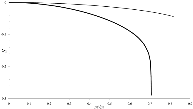
Figure 2: Electroweak $S$ parameter from left-handed doublet and triplet scalars: thick solid line, left-handed triplet; thin solid line, left-handed doublet.

Since the $S$ parameters in Fig. 2 are bounded from above, at $\beta=0$, the contribution from the scalars of the theory is net negative. The total contribution from the scalar fields to $S$, however, is a sum of all scalar contributions. As the $\beta$ parameter for each scalar multiplet is not known, we may only speak of the bounds the total scalar contribution should lie within, namely

$$0\geqslant S_{\mathrm{scalars}}\geqslant-3.13\,\,.$$ (81)

To be inclusive, we may also consider the contribution from a heavy SM model Higgs to $S$, which can be positive depending on its mass. This contribution, however, is relatively small even for an exotic Higgs with 1 TeV mass, where it can reach up to 0.06. With such contribution, if heavy SM Higgs exists at all, it would not change the maximum negative $S$ provided by other scalars, significantly. On the other hand, the fermionic contribution to $S$ from three generations of unconventional fermions is within

$$1.17\geqslant S_{\mathrm{fermions}}\geqslant 0.58\,\,.$$ (82)

The positive contribution from unconventional fermions obviously violates the experimental bounds. Nonetheless, the negative scalar contribution to $S$ has the potential to bring the total $S$ in agreement with the experimental constraint on new physics, given in Eq. (77a). Therefore, the notion of three extra generations of heavy fermions can, in principal, be accommodated within the model.

VII The decay of unconventional fermions

Although unconventional fermions can have transitions involving ordinary fermions via $\mathrm{SU}(4)_{\mathrm{PS}}$ and $\mathrm{SU}(3)_{H}$ mediated processes, the lightest unconventional fermion cannot decay into light ordinary fermions, even through weak channels. That poses an alarming danger: a stable unconventional fermion. There are stringent constraints on heavy stable fermions (quarks or leptons) from cosmology (e.g., nucleosynthesis) and earth-based experiments. Those constraints are discussed in length in Ref. Frampton et al. (2000) and the references therein.

Fortunately, the decay of the lightest unconventional fermion is possible via the mixing among the charged gauge bosons. Such mixing is possible through $\Theta$’s VEV, which mixes the charged gauge bosons $W_{\mu H}^{\pm}$ and $W_{\mu L}^{\pm}$, since it carries $\mathrm{SU}(2)_{L}$ and $\mathrm{SU}(2)_{H}$ quantum numbers. This mixing has been discussed in Appendix A, where its rather long expressions are given for completeness.

The mixing between the charged gauge bosons corresponds to an equivalent mixing among the relevant currents as well. If we denote gauge eigenstates of charged bosons by $W_{\mu H}^{\pm}$ and $W_{\mu L}^{\pm}$, and mass eigenstates by $\tilde{W}_{\mu H}^{\pm}$ and $\tilde{W}_{\mu L}^{\pm}$, we may write (to first approximation)

$$\tilde{W}_{\mu L}^{\pm}=W_{\mu L}^{\pm}+\mathcal{O}\left({\frac{{v^{2}}}{{v_{H}^{{}^{\prime}2}}}}\right)W_{\mu H}^{\pm}\,,$$ (83a)

$$\tilde{W}_{\mu H}^{\pm}=W_{\mu H}^{\pm}+\mathcal{O}\left({\frac{{v^{2}}}{{v_{H}^{{}^{\prime}2}}}}\right)W_{\mu L}^{\pm}\,,$$ (83b)

where $v$ and $v^{\prime}_{H}$ are the VEV’s of the SM Higgs $H$, and the horizontal breaking Higgs $\Phi_{H}^{\left(2\right)}$, respectively. Let us also denote currents coupled to gauge eigenstates by $J_{\mu H}$ and $J_{\mu L}$, and those coupled to mass eigenstates by $\tilde{J}_{\mu H}$ and $\tilde{J}_{\mu L}$. The same matrix that connects the gauge and mass eigenstate charged bosons relates the corresponding currents to each other as well. Therefore, we have

$$\tilde{J}_{\mu L} =J_{\mu L}+\mathcal{O}\left({\frac{{v^{2}}}{{v_{H}^{{}^{\prime}2}}}}\right)J_{\mu H}\,,$$ (84a)

$$\tilde{J}_{\mu H} =J_{\mu H}+\mathcal{O}\left({\frac{{v^{2}}}{{v_{H}^{{}^{\prime}2}}}}\right)J_{\mu L}\,.$$ (84b)

The consequent interaction terms are then given by

$$\mathcal{L}_{L}=g_{W}\tilde{J}_{L}^{\mu}\tilde{W}_{\mu L}=g_{W}\left[{J_{L}^{\mu}+\mathcal{O}\left({\frac{{v^{2}}}{{v_{H}^{{}^{\prime}2}}}}\right)J_{H}^{\mu}}\right]\tilde{W}_{\mu L},$$ (85a)

and

$$\mathcal{L}_{H}=g_{W}\tilde{J}_{H}^{\mu}\tilde{W}_{\mu H}=g_{W}\left[{J_{H}^{\mu}+\mathcal{O}\left({\frac{{v^{2}}}{{v_{H}^{{}^{\prime}2}}}}\right)J_{L}^{\mu}}\right]\tilde{W}_{\mu H}.$$ (85b)

The interaction term of Eq. (85a) portrays how the lightest unconventional fermion, in $J_{\mu H}$, can couple to $\tilde{W}_{\mu L}^{\pm}$ and therefore decay into ordinary fermions. The decay mechanism falls within one of the two possibilities:

1. The mass of the lightest unconventional fermion is large enough to decay into a real $\tilde{W}_{L}$ and a regular fermion, according to $g_{W}\mathcal{O}\left({{{v^{2}}\mathord{\left/{\vphantom{{v^{2}}{v_{H}^{{}^{\prime}2}}}}\right.\kern-1.2pt}{v_{H}^{{}^{\prime}2}}}}\right)J_{H}^{\mu}\tilde{W}_{\mu L}$. Although the $\mathcal{O}\left({{{v^{2}}\mathord{\left/{\vphantom{{v^{2}}{v_{H}^{{}^{\prime}2}}}}\right.\kern-1.2pt}{v_{H}^{{}^{\prime}2}}}}\right)$ factor is small, the corresponding decay rate can be sizeable, since the unconventional fermion decays into a real $\tilde{W}_{L}$.

2. The mass of the lightest unconventional fermion is not large enough to decay into a real $\tilde{W}_{L}$ and a regular fermion. In that case, $\tilde{W}_{L}$ would be virtual and the interaction involves a $\tilde{W}_{L}$ propagator, i.e.,

   $$\mathcal{L}_{\mathrm{int}}\sim g_{W}^{2}\mathcal{O}\left({\frac{{v^{2}}}{{v_{H}^{{}^{\prime}2}}}}\right)J_{L}^{\mu\dagger}\frac{{1}}{{p^{2}-M_{\tilde{W}_{L}}^{2}}}J_{\mu H}.$$

The fermions appearing in $J_{\mu L}$ and $J_{\mu H}$ should be expressed in terms of mass eigenstates. This means new mixing angels, which are totally different from the known CKM matrix elements. Thus, the computation of the lifetimes of unconventional fermions involves unknown mixing angels; one could only have a rational estimate for.

To estimate the lifetime and decay length of the lightest unconventional fermion, which is the long-lived one, we note that the dominant decay is that into a real $\tilde{W}_{L}$. For illustration purposes, let us assume that the lightest unconventional quark and lepton are $D$ and $l_{d}$, respectively. Their dominant decay modes would be

$$D\left(-{\frac{4}{3}}\right)\to d^{j}\left(-{\frac{1}{3}}\right)+\tilde{W}_{L}^{-},$$ (86a)

$$l_{d}\left(1\right)\to\nu^{k}\left(0\right)+\tilde{W}_{L}^{+},$$ (86b)

where $j=d,s,b$, and $k=e,\mu,\tau$, and all fermions ought to be mass eigenstates. The decay widths can be found easily. For $m_{d^{j},\nu^{k}}\ll m_{D,l_{d}}$ , the decay widths are simply given by

$$\Gamma_{D}=\frac{{G_{F}m_{D}^{3}}}{{8\pi\sqrt{2}}}\left|{\mathcal{O}\left({\frac{{v^{2}}}{{v_{H}^{{}^{\prime}2}}}}\right)}\right|^{2}\left|{V_{Q}}\right|^{2}\left({1+\frac{{2M_{\tilde{W}_{L}}^{2}}}{{m_{D}^{2}}}}\right)\left({1-\frac{{M_{\tilde{W}_{L}}^{2}}}{{m_{D}^{2}}}}\right)^{2},$$ (87a)

$$\Gamma_{l_{d}}=\frac{{G_{F}m_{l_{d}}^{3}}}{{8\pi\sqrt{2}}}\left|{\mathcal{O}\left({\frac{{v^{2}}}{{v_{H}^{{}^{\prime}2}}}}\right)}\right|^{2}\left|{V_{L}}\right|^{2}\left({1+\frac{{2M_{\tilde{W}_{L}}^{2}}}{{m_{l_{d}}^{2}}}}\right)\left({1-\frac{{M_{\tilde{W}_{L}}^{2}}}{{m_{l_{d}}^{2}}}}\right)^{2}.$$ (87b)

The factors $V_{Q}$ and $V_{L}$ are the relevant elements of matrices $V_{Q}=\mathrm{U}_{D}^{-1}\mathrm{U}_{U}$ and $V_{L}=\mathrm{U}_{l_{d}}^{-1}\mathrm{U}_{l_{u}}$, which describe the mixings among the unconventional quarks and leptons, respectively. To be precise, $\mathrm{U}_{U}$, $\mathrm{U}_{D}$ and $\mathrm{U}_{l_{u}}$, $\mathrm{U}_{l_{d}}$ are matrices which diagonalize the up-, down-sector of unconventional quarks and leptons, respectively. To obtain an estimate, let us take a rational value for the masses of $D$ and $l_{d}$, namely $m_{D}\approx m_{l_{d}}\approx 250$ GeV and apply realistic assumption $\mathcal{O}\left({{{v^{2}}\mathord{\left/{\vphantom{{v^{2}}{v_{H}^{{}^{\prime}2}}}}\right.\kern-1.2pt}{v_{H}^{{}^{\prime}2}}}}\right)\approx 10^{-2}$. Then typical lifetimes for the lightest unconventional fermions can be estimated

$$\tau_{D}\approx 1.3\times 10^{-21}\left|{V_{Q}}\right|^{-2}\,\,\mathrm{s}\,,$$ (88a)

$$\tau_{l_{d}}\approx 1.3\times 10^{-21}\left|{V_{L}}\right|^{-2}\,\,\mathrm{s}\,.$$ (88b)

These lifetimes are obviously short, which indicate that unconventional fermions decay fast and therefore pose no cosmological problems, unless the mixing factors are peculiarly small. A typical decay length for the lightest unconventional quark and lepton can also be estimated from the lifetimes of Eqs. (88), they are

$$l_{D}\approx 400\left|{V_{Q}}\right|^{-2}\,\,\mathrm{fm}\,,$$ (89a)

$$l_{l_{d}}\approx 400\left|{V_{L}}\right|^{-2}\,\,\mathrm{fm}\,,$$ (89b)

which also depend on the mixings $V_{Q}$ and $V_{L}$. To summarize, we showed that the lightest of unconventional quarks or leptons will not be stable and can decay through the mixing among the horizontal and left-handed charged gauge bosons. Very short lifetimes (for reasonably small mixings) are possible for the longest-lived unconventional fermions, which alleviate cosmological concerns on heavy stable fermions.

VIII Summary

We examined the idea of early quark-lepton mass unification through one of petite unification models $\mathrm{PUT}_{2}=\mathrm{SU}(4)_{\mathrm{PS}}\otimes\mathrm{SU}(3)_{L}\otimes\mathrm{SU}(3)_{H}$.

For this we embedded $\mathrm{PUT}_{2}$ into a 5D model, in brane world picture. The petite unification scenario calls for new chiral fermions with unconventional charges. The philosophy was that the sizes of 4D couplings in chiral fermion mass terms are controlled by the left-right overlaps between the corresponding localized fermions along the extra dimension. The magnitudes of these overlaps are set by the geometry of the localized zero modes in the extra dimension. We chose to establish such geometry by reducing the symmetry of the model to that of the SM. This way the quark-lepton unification structure translates into the geometry of the localized zero modes and yields a quark-lepton mass unification structure. This idea therefore sets the symmetry breakings along the extra dimension in motion systematically.

As a result, the effective Yukawa couplings of quarks and leptons even those of unconventional fermions and the SM fermions relate to each other. A numerical estimation of mass scales showed that the unconventional fermion mass scales can set bounds on the mass scales of Dirac neutrino and vice versa. For example, light unconventional fermions (up to 500 GeV mass scales) set 1 eV bound on neutrino mass scale, which imply a near-degenerate mass matrix for neutrino sector. On the other hand, lighter unconventional fermions (as light as 180 GeV) yield light (less than 0.1 eV) neutrino sector, which corresponds to a hierarchical or near-degenerate mass matrix for neutrinos.

The mass scales obtained in this model are similar to those of $\mathrm{PUT}_{1}$. The strong $\mathrm{SU}(4)_{\mathrm{PS}}$ is the common group of PUT scenarios. The unconventional quarks and leptons are connected to their normal siblings through the quartets of this group in both scenarios. Breaking $\mathrm{SU}(4)_{\mathrm{PS}}$ along the extra dimension results in similar relations between the left-right separations of quarks and leptons and that translates into similar mass scales for both models.

We computed the contributions of extra heavy fermions and scalars of the model to the electroweak oblique parameter S, and showed that the extra generations of heavy fermions may not violate the experimental bounds on new physics, in principle.

The issue of the decay of the lightest unconventional fermion was also discussed. We showed that the lightest unconventional fermion is indeed unstable, as it decays to ordinary fermions through the mixing of charged gauge bosons. The estimated lifetimes for the lightest unconventional quark and lepton also appeared to be small enough to comply with the cosmological bounds on stable heavy fermions.

In addition, we discussed the gauge symmetry breaking of the model in length, where the mixings of neutral and charged gauge bosons of the model were explained explicitly.

Appendix A The gauge symmetry breakdown of the model

In this appendix, we describe the gauge symmetry breaking of our model in 4D space down to $\mathrm{SU}(3)_{c}\otimes\mathrm{U}(1)_{EM}$. We follow the gauge symmetry breaking pattern given in section II, Eqs. (3), and describe the symmetry breakings, as usual, by scalar Higgs fields with non-zero VEV’s.

A.1 Strong breakdown

The strong breakdown of $\mathrm{PUT}_{2}$, at energy scale $M$, can be accomplished by a Higgs-field multiplet, which we denote by $\Phi_{\mathrm{PS}}=\left({15,1,1}\right)$. The VEV of this Higgs field, must leave the QCD gauge group unbroken, decouple the color quark triplet from the lepton color singlet in the $\mathrm{SU}(4)_{\mathrm{PS}}$ fundamental representation, and give mass to six intermediate (lepto-quark) gauge bosons of $\mathrm{SU}(4)_{\mathrm{PS}}$ symmetry. The lepto-quark gauge bosons in terms of $\mathrm{SU}(4)_{\mathrm{PS}}$ gauge bosons $A_{\mu S}^{j}$ are

$$\begin{gathered}X_{\mu 1}^{\pm}=\frac{1}{{\sqrt{2}}}\left({A_{\mu S}^{9}\mp iA_{\mu S}^{10}}\right)\,,\hfill\\ X_{\mu 2}^{\pm}=\frac{1}{{\sqrt{2}}}\left({A_{\mu S}^{11}\mp iA_{\mu S}^{12}}\right)\,,\hfill\\ X_{\mu 3}^{\pm}=\frac{1}{{\sqrt{2}}}\left({A_{\mu S}^{13}\mp iA_{\mu S}^{14}}\right)\,.\hfill\\ \end{gathered}$$ (90)

They carry electric charge $\pm{4\mathord{\left/{\vphantom{43}}\right.\kern-1.2pt}3}$ and receive mass from the VEV of $\Phi_{\mathrm{P}S}$. The covariant derivative of $\mathrm{SU}(4)_{\mathrm{PS}}\otimes\mathrm{SU}(3)_{L}\otimes\mathrm{SU}(3)_{H}$ is

$$\hat{D}_{\mu}=\partial_{\mu}+ig_{S}\hat{A}_{\mu S}+ig_{W}\hat{A}_{\mu L}+ig_{W}\hat{A}_{\mu H}\,,$$ (91)

where $\hat{A}_{\mu S}=\sum\limits_{j=1}^{15}{\hat{T}_{j}}A_{\mu S}^{j}$ and $\hat{A}_{\mu L,H}=\sum\limits_{j=1}^{8}{\hat{F}_{j}}A_{\mu L,H}^{j}$ with $\hat{T}_{j}$ and $\hat{F}_{j}$ being the generators of $\mathrm{SU}(4)$ and $\mathrm{SU}(3)$ algebras. The lepto-quark mass terms come from the kinetic energy of the Higss field $\Phi_{\mathrm{PS}}$, i.e.,

$$\mathcal{L}_{\Phi_{\mathrm{PS}},\mathrm{kin}}=\mathrm{Tr}\left({\left|{D_{\mu}\Phi_{\mathrm{PS}}}\right|^{2}}\right)=\frac{1}{2}\mathrm{Tr}\left({\left|{\partial_{\mu}\Phi_{\mathrm{PS}}+ig_{S}\left[{\hat{A}_{\mu S},\Phi_{\mathrm{PS}}}\right]}\right|^{2}}\right).$$ (92)

Once $\Phi_{\mathrm{PS}}$ attains VEV

$$\left\langle{\Phi_{PS}}\right\rangle=v_{PS}\left({\begin{array}[]{*{20}c}{\frac{1}{3}}&0&0&0\\ 0&{\frac{1}{3}}&0&0\\ 0&0&{\frac{1}{3}}&0\\ 0&0&0&{-1}\\ \end{array}}\right)\,,$$ (93)

the lepto-quark gauge bosons receive mass in the form

$$\mathcal{L}_{X,\mathrm{mass}}=\frac{4}{9}g_{S}^{2}v_{PS}^{2}\sum\limits_{j=1}^{3}{\left|{X_{\mu j}}\right|^{2}}=M_{X}^{2}\sum\limits_{j=1}^{3}{\left|{X_{\mu j}}\right|^{2}},$$ (94)

where $M_{X}={{2g_{S}v_{PS}}\mathord{\left/{\vphantom{{2g_{S}v_{S}}3}}\right.\kern-1.2pt}3}$ and $j$ refers to the color degree of freedom.

A.2 Weak breakdown

Right above the next symmetry breaking scale $\tilde{M}$, the gauge group that needs to be broken is $\mathrm{U}(1)_{S}\otimes\mathrm{SU}(3)_{L}\otimes\mathrm{SU}(3)_{H}$. The breaking of this group should furnish the generator of the SM’s weak hypercharge group $\hat{Y}_{W}=C_{S}\hat{T}_{15\mathrm{PS}}+C_{L}\hat{T}_{8L}+C_{1H}\hat{T}_{8H}+C_{2H}\hat{T}_{3H}$. This means that at least one of the Higgs fields for such breaking must have non-vanishing $\mathrm{U}(1)_{S}$ quantum number. The breaking of $\mathrm{SU}(3)_{L}$ into $\mathrm{SU}(2)_{L}\otimes\mathrm{U}(1)_{L}$ can be done by the Higgs field $\Phi_{L}=\left({1,8,1}\right)$. The VEV of $\Phi_{L}$ should decouple the left-handed doublet from the singlet in $\mathrm{SU}(3)_{L}$ fundamental representation [see, e.g., Eqs. (13)] and give mass to four intermediate gauge bosons of $\mathrm{SU}(3)_{L}$ symmetry. Therefore, its VEV should take on the eighth direction of the multiplet. The intermediate gauge bosons can be written in terms of $\mathrm{SU}(3)_{L}$ gauge fields $A_{\mu L}^{j}$, i.e.,

$$\begin{gathered}V_{\mu 1}^{\pm}=\frac{1}{{\sqrt{2}}}\left({A_{\mu L}^{4}\mp iA_{\mu L}^{5}}\right),\hfill\\ V_{\mu 2}^{\pm}=\frac{1}{{\sqrt{2}}}\left({A_{\mu L}^{6}\mp iA_{\mu L}^{7}}\right).\hfill\\ \end{gathered}$$ (95)

The covariant derivative of $\mathrm{SU}(3)_{c}\otimes\mathrm{SU}(3)_{L}\otimes\mathrm{SU}(3)_{H}\otimes\mathrm{U}(1)_{S}$ is

$$\hat{D}_{\mu}=\partial_{\mu}+ig_{3}\hat{G}_{\mu}+ig_{W}\hat{A}_{\mu L}+ig_{W}\hat{A}_{\mu H}+i\tilde{g}_{S}\hat{Y}_{S}\tilde{A}_{\mu S}\,,$$ (96)

where $G_{\mu}^{j}$ are gluon fields and $\tilde{A}_{\mu S}$ is the neutral gauge boson of $\mathrm{U}(1)_{S}$. As usual, the mass terms of $V_{\mu j}^{\pm}$ come from the kinetic energy of $\Phi_{L}$, which is in the form $\mathrm{Tr}\left({\left|{D_{\mu}\Phi_{L}}\right|^{2}}\right)$. With $\Phi_{L}$ taking VEV in the form

$$\left\langle{\Phi_{L}}\right\rangle=v_{L}\left({\begin{array}[]{*{20}c}1&0&0\\ 0&1&0\\ 0&0&{-2}\\ \end{array}}\right)\,,$$ (97)

the mass of $V_{\mu j}$ fields easily turns out to be $M_{V}={{3g_{W}v_{L}}\mathord{\left/{\vphantom{{3g_{W}v_{L}}2}}\right.\kern-1.2pt}2}$.

The symmetry breaking of $\mathrm{SU}(3)_{H}$, on the other hand, needs to have non-vanishing $\mathrm{U}(1)_{S}$ and $\mathrm{U}(1)_{L}$ quantum numbers, so that at the end three of four neutral gauge bosons acquire masses and the weak hypercharge gauge boson, $B_{\mu}$, emerges as a massless field. One economical scenario for $\mathrm{SU}(3)_{H}$ symmetry breaking in two steps can consist of Higgs field multiplets $\Phi^{(1)}_{H}=\left({1,1,8}\right)$ and $\Phi^{(2)}_{H}=\left({4,3,3}\right)$. In the first step, $\Phi^{(1)}_{H}$ breaks $\mathrm{SU}(3)_{H}$ into $\mathrm{SU}(2)_{H}\otimes\mathrm{U}(1)_{H}$ and then $\Phi^{(2)}_{H}$ destroys the horizontal symmetry completely. The VEV of $\Phi^{(1)}_{H}$ should take on the eighth direction of the multiplet to decouple $\mathrm{SU}(2)_{H}$ and $\mathrm{U}(1)_{H}$ subgroups. In addition, $\Phi^{(1)}_{H}$’s VEV gives mass to four intermediate gauge bosons of $\mathrm{SU}(3)_{H}$ symmetry. These are the gauge bosons, which connect SM-type fermions to vector-like fermions. They can be written in terms of the horizontal gauge bosons $A_{\mu H}^{j}$, as

$$\begin{gathered}U_{\mu 1}^{\pm}=\frac{1}{{\sqrt{2}}}\left({A_{\mu H}^{4}\mp iA_{\mu H}^{5}}\right),\hfill\\ U_{\mu 2}^{\pm}=\frac{1}{{\sqrt{2}}}\left({A_{\mu H}^{6}\mp iA_{\mu H}^{7}}\right).\hfill\\ \end{gathered}$$ (98)

The VEV of $\Phi_{H}^{\left(1\right)}$ takes the same form as that of $\Phi_{L}$, but in horizontal space. Therefore, the mass of $U_{\mu j}$ bosons simply reads $M_{U}={{3g_{W}v_{H}}\mathord{\left/{\vphantom{{3g_{W}v_{H}}2}}\right.\kern-1.2pt}2}$, where $v_{H}$ is the amplitude of $\Phi_{H}^{\left(1\right)}$’s VEV.

To complete horizontal symmetry breaking, $\Phi^{(2)}_{H}$ will develop VEV, which must be on its colorless component to preserve QCD symmetry. In order to keep $\mathrm{SU}(2)_{L}$ symmetry intact, $\Phi^{(2)}_{H}$’s VEV should also be on the singlet component of its $\mathrm{SU}(3)_{L}$ triplet. Finally to destroy $\mathrm{SU}(2)_{H}$, the horizontal triplet of $\Phi^{(2)}_{H}$ simply attains VEV in its doublet in the form $\bigl{(}\begin{smallmatrix}0\\ {{{v^{\prime}_{H}}\mathord{\left/{\vphantom{{v^{\prime}_{H}}{\sqrt{2}}}}\right.\kern-1.2pt}{\sqrt{2}}}}\end{smallmatrix}\bigl{)}$. In the process of destroying $\mathrm{SU}(2)_{H}$ symmetry, the four unbroken neutral gauge bosons will mix and as a result we end up with three massive and one massless gauge bosons. The massless gauge boson $B_{\mu}$, corresponds to $\mathrm{U}(1)_{Y}$ symmetry. The $\mathrm{SU}(2)_{H}$ symmetry has three gauge bosons: $W_{\mu H}^{\pm}$ and $W_{\mu H}^{3}$. The charged gauge bosons receive mass through the kinetic energy term of $\Phi_{H}^{\left(2\right)}$, which turns out to be $M_{W_{H}}={{g_{W}v^{\prime}_{H}}\mathord{\left/{\vphantom{{g_{W}v^{\prime}_{H}}{\sqrt{2}}}}\right.\kern-1.2pt}{\sqrt{2}}}$. The mixing of the neutral gauge bosons $\tilde{A}_{\mu S}$, $\tilde{A}_{\mu L}$, $\tilde{A}_{\mu H}$, $W_{\mu H}^{3}$ is through the VEV of $\Phi_{H}^{\left(2\right)}$, i.e.,

$$\left\langle{\Phi_{H}^{\left(2\right)}}\right\rangle=\left({\begin{array}[]{*{20}c}0\\ 0\\ 0\\ 1\\ \end{array}}\right)\otimes\left({\begin{array}[]{*{20}c}0\\ 0\\ 1\\ \end{array}}\right)\otimes\left({\begin{array}[]{*{20}c}0\\ {\tfrac{{v^{\prime}_{H}}}{{\sqrt{2}}}}\\ 0\\ \end{array}}\right).$$ (99)

The kinetic energy of $\Phi_{H}^{\left(2\right)}$ is

$$\mathcal{L}_{\Phi_{H}^{\left(2\right)},\mathrm{kin}}=\mathrm{Tr}\left[{\left|{\left({\partial_{\mu}+ig_{W}\hat{W}_{\mu H}-\frac{{ig_{W}}}{{3\sqrt{3}}}\hat{A}_{\mu L}+\frac{{ig_{W}}}{{6\sqrt{3}}}\hat{A}_{\mu H}-i\sqrt{\frac{3}{8}}\tilde{g}_{S}\hat{Y}_{S}\tilde{A}_{\mu S}}\right)\Phi_{H}^{\left(2\right)}}\right|^{2}}\right],$$ (100)

where $\hat{W}_{\mu H}=\sum\limits_{j=1}^{3}{W_{\mu H}^{j}}\hat{T}_{j}$. The squared mass matrix of neutral gauge bosons is obtained from the above trace, i.e.,

$$M^{2}=\left({\begin{array}[]{*{20}c}{\frac{3}{4}g_{W}^{2}v^{\prime 2}_{H}}&{-\frac{1}{{12\sqrt{6}}}g_{W}^{2}v^{\prime 2}_{H}}&{\frac{1}{{6\sqrt{6}}}g_{W}^{2}v^{\prime 2}_{H}}&{\frac{{\sqrt{3}}}{8}g_{W}\tilde{g}_{S}v^{\prime 2}_{H}}\\ {-\frac{1}{{12\sqrt{6}}}g_{W}^{2}v^{\prime 2}_{H}}&{\frac{1}{{216}}g_{W}^{2}v^{\prime 2}_{H}}&{-\frac{1}{{108}}g_{W}^{2}v^{\prime 2}_{H}}&{-\frac{1}{{24\sqrt{2}}}g_{W}\tilde{g}_{S}v^{\prime 2}_{H}}\\ {\frac{1}{{6\sqrt{6}}}g_{W}^{2}v^{\prime 2}_{H}}&{-\frac{1}{{108}}g_{W}^{2}v^{\prime 2}_{H}}&{\frac{1}{{54}}g_{W}^{2}v^{\prime 2}_{H}}&{\frac{1}{{12\sqrt{2}}}g_{W}\tilde{g}_{S}v^{\prime 2}_{H}}\\ {\frac{{\sqrt{3}}}{8}g_{W}\tilde{g}_{S}v^{\prime 2}_{H}}&{-\frac{1}{{24\sqrt{2}}}g_{W}\tilde{g}_{S}v^{\prime 2}_{H}}&{\frac{1}{{12\sqrt{2}}}g_{W}\tilde{g}_{S}v^{\prime 2}_{H}}&{\frac{3}{{16}}\tilde{g}_{S}^{2}v^{\prime 2}_{H}}\\ \end{array}}\right).$$ (101)

The mass terms would look like

$$\left({\begin{array}[]{*{20}c}{W_{\mu H}^{3}}&{\tilde{A}_{\mu H}}&{\tilde{A}_{\mu L}}&{\tilde{A}_{\mu S}}\\ \end{array}}\right)M^{2}\left({\begin{array}[]{*{20}c}{W_{\mu H}^{3}}\\ {\tilde{A}_{\mu H}}\\ {\tilde{A}_{\mu L}}\\ {\tilde{A}_{\mu S}}\\ \end{array}}\right).$$ (102)

The squared mass matrix can be diagonalized, which leaves one massless gauge boson, $B^{\mu}$. The eigenvector corresponding to the zero eigenvalue is (after normalization)

$$B_{\mu}=\frac{1}{{\sqrt{15g_{W}^{2}+453\tilde{g}_{S}^{2}}}}\left({-4\sqrt{3}\tilde{g}_{S}W_{\mu H}^{3}+\frac{{27\tilde{g}_{S}}}{{\sqrt{5}}}\tilde{A}_{\mu H}+\frac{{36\tilde{g}_{S}}}{{\sqrt{5}}}\tilde{A}_{\mu L}+4g_{W}\tilde{A}_{\mu S}}\right).$$ (103)

A.3 The SM breakdown and fermion masses

To break $\mathrm{PUT}_{2}$’s gauge group further down to $\mathrm{SU}(3)_{c}\otimes\mathrm{U}(1)_{EM}$, we need another Higgs field, which in addition to the symmetry breaking is also responsible for giving mass to all SM-type fermions of the model. The mass terms for SM-type fermions involve couplings of left-handed and right-handed fields with a Higgs field, which develops VEV. To achieve this in our model, we need to couple $\Psi_{1}$ to itself and also to $\Psi_{2}$ through appropriate Higgs fields.

The SM Higgs field transforms as $(2,1)$ under $\mathrm{SU}(2)_{L}\otimes\mathrm{U}(1)_{Y}$. Therefore, the $\mathrm{SU}(3)_{L}$ representation of a Higgs multiplet that breaks the SM, must contain a $(2,1)$. The SM symmetry breakdown, then, is through the VEV of a Higgs multiplet transforming as $\Theta=\left(1,8,8\right)$. The decomposition of $\Theta$’s $\mathrm{SU}(3)_{L}$ octet, in terms of $\mathrm{SU}(2)_{L}\otimes\mathrm{U}(1)_{Y}$ multiplets or quantum numbers, yields

$$\left[8\right]_{\mathrm{SU}\left(3\right)_{L}}=\left(3,0\right)\oplus\left(2,1\right)\oplus\left(2,-1\right)\oplus\left(1,0\right),$$ (104)

which in matrix form can be written as

$$\left({\begin{array}[]{*{20}c}{\left({3,0}\right)}&\vline&{\left({2,1}\right)}\\ \hline\cr{\left({2,-1}\right)}&\vline&{\left({1,0}\right)}\\ \end{array}}\right).$$ (105)

Therefore, $\Theta$ contains a SM Higgs field, which we denote by $H=(2,1)$, and should develop a VEV in $H$. The decomposition of $\Theta$’s horizontal octet is essentially the same as that of the $\mathrm{SU}(3)_{L}$ octet, but in terms of multiplets or quantum numbers of $\mathrm{SU}(2)_{H}\otimes\mathrm{U}(1)_{H}$. To avoid vector-like fermions receiving mass through the SM’s Higgs the horizontal octet cannot contribute to $\Theta$’s VEV in its $(1,0)$ part and must have a vanishing $\mathrm{U}(1)_{H}$ quantum number. This means that the horizontal contribution to $\Theta$’s VEV can only exist in the $(3,0)$ part.

Through the kinetic energy term, $\Theta$’s VEV breaks the SM symmetry down to $\mathrm{SU}(3)_{c}\otimes\mathrm{U}(1)_{EM}$, and gives mass to $W^{\pm}$ and $Z^{0}$. In addition, $\Theta$’s VEV mixes the charged gauge bosons, $W_{\mu H}^{\pm}$ and $W_{\mu L}^{\pm}$, since it carries $\mathrm{SU}(2)_{L}$ and $\mathrm{SU}(2)_{H}$ quantum numbers. To be precise, such mixing of “gauge eigenstates” yields new charged gauge bosons which we may call “mass eigenstates.” Let us denote the mass eigenstates of such mixing by $\tilde{W}_{\mu H}^{\pm}$ and $\tilde{W}_{\mu L}^{\pm}$. They can easily be expressed in terms of the gauge eigenstates, $W_{\mu H}^{\pm}$ and $W_{\mu L}^{\pm}$ (and vice versa). The squared mass matrix of charged gauge bosons, similar to neutral gauge boson mixing, can be diagonalized by an orthogonal matrix, $R$. Such matrix connects the mass eigenstates, $\tilde{W}_{\mu H}^{\pm}$, $\tilde{W}_{\mu L}^{\pm}$, and gauge eigenstates, $W_{\mu H}^{\pm}$, $W_{\mu L}^{\pm}$, i.e.,

$$\left({\begin{array}[]{*{20}c}{\tilde{W}_{\mu L}^{\pm}}\\ {\tilde{W}_{\mu H}^{\pm}}\\ \end{array}}\right)=R\left({\begin{array}[]{*{20}c}{W_{\mu L}^{\pm}}\\ {W_{\mu H}^{\pm}}\\ \end{array}}\right),$$ (106)

and vice versa

$$\left({\begin{array}[]{*{20}c}{W_{\mu L}^{\pm}}\\ {W_{\mu H}^{\pm}}\\ \end{array}}\right)=R^{T}\left({\begin{array}[]{*{20}c}{\tilde{W}_{\mu L}^{\pm}}\\ {\tilde{W}_{\mu H}^{\pm}}\\ \end{array}}\right).$$ (107)

The unnormalized mass eigenvectors and their masses are given by

$$\begin{aligned} \tilde{W}_{\mu L}^{\pm}=&W_{\mu L}^{\pm}-\left[{\frac{{\left({g_{W}^{2}-g_{2}^{2}}\right)}}{{g_{W}g_{2}}}\frac{{v^{2}}}{{v_{H}^{2}}}}\right.\hfill\\ &\left.{+\frac{{\sqrt{\left[{\left({g_{W}^{2}-g_{2}^{2}}\right)\frac{{v^{2}}}{{v_{H}^{2}}}+g_{W}^{2}}\right]^{2}+4\left[{\left({g_{W}g_{2}-g_{W}^{2}g_{2}^{2}}\right)\frac{{v^{4}}}{{v_{H}^{4}}}-g_{W}^{2}g_{2}^{2}\frac{{v^{2}}}{{v_{H}^{2}}}}\right]}}}{{g_{W}g_{2}}}}\right]W_{\mu H}^{\pm}\hfill\\ \end{aligned}$$ (108a)

with

$$M_{\tilde{W}_{L}}=\left[{\frac{{\left({g_{2}^{2}+g_{W}^{2}}\right)v^{2}+g_{W}^{2}v^{\prime 2}_{H}+\sqrt{\left({g_{2}^{2}+g_{W}^{2}}\right)^{2}v^{4}+g_{W}^{4}v^{\prime 4}_{H}+2\left({g_{W}^{2}-g_{2}^{2}}\right)v^{2}v^{\prime 2}_{H}}}}{4}}\right]^{\frac{1}{2}}\,,$$ (108b)

and

$$\begin{aligned} \tilde{W}_{\mu H}^{\pm}=&W_{\mu H}^{\pm}-\left[{\frac{{\left({g_{W}^{2}-g_{2}^{2}}\right)}}{{g_{W}g_{2}}}\frac{{v^{2}}}{{v_{H}^{2}}}}\right.\hfill\\ &\left.{-\frac{{\sqrt{\left[{\left({g_{W}^{2}-g_{2}^{2}}\right)\frac{{v^{2}}}{{v_{H}^{2}}}+g_{W}^{2}}\right]^{2}+4\left[{\left({g_{W}g_{2}-g_{W}^{2}g_{2}^{2}}\right)\frac{{v^{4}}}{{v_{H}^{4}}}-g_{W}^{2}g_{2}^{2}\frac{{v^{2}}}{{v_{H}^{2}}}}\right]}}}{{g_{W}g_{2}}}}\right]W_{\mu L}^{\pm}\hfill\\ \end{aligned}$$ (109a)

with

$$M_{\tilde{W}_{H}}=\left[{\frac{{\left({g_{2}^{2}+g_{W}^{2}}\right)v^{2}+g_{W}^{2}v^{\prime 2}_{H}-\sqrt{\left({g_{2}^{2}+g_{W}^{2}}\right)^{2}v^{4}+g_{W}^{4}v^{\prime 4}_{H}+2\left({g_{W}^{2}-g_{2}^{2}}\right)v^{2}v^{\prime 2}_{H}}}}{4}}\right]^{\frac{1}{2}}.$$ (109b)

Dirac mass terms, involving the left- and right-handed SM-type fermions, can be written in the form

$$\mathcal{L}_{\mathrm{mass}}=\kappa_{1}\Psi_{1}^{T}\Theta C\Psi_{2}^{\ast}+\kappa_{2}\Psi_{1}^{T}\tilde{\Theta}C\Psi_{1}^{\ast}+h.c.\;,$$ (110)

where $C$ is is the charge conjugation operator $C=i\gamma^{2}\gamma^{0}$; $\kappa_{1}$ and $\kappa_{2}$ can be different in general, and $\tilde{\Theta}=i\hat{\lambda}_{2L}\Theta^{*}$. One notices $i\hat{\lambda}_{2L}$ in $\tilde{\Theta}$, which analogous to the presence of $i\hat{\tau}_{2}$ in the SM’s quark mass terms.

The mass terms in Eq. (110) are rather compact. To convince ourselves that they yield correct mass terms for SM-type fermions, let us expand them for at least one flavor doublet. As explained, $\Theta$’s VEV has two parts: an $\mathrm{SU}(3)_{L}$ octet, which contains the SM Higgs, and a horizontal octet. The horizontal octet in $\Theta$’s VEV eliminates purely vector-like left-handed triplets (e.g., those in Eqs.(13b and 16b)) and therefore prevents them from receiving mass from the SM Higgs VEV. Thus, the only left-handed triplets that stay in play are those which involve SM-type fermions. Of those, let us consider $\Psi_{1}$’s

$$\left({\begin{array}[]{*{20}c}{d_{L}^{*}}\\ {-u_{L}^{*}}\\ {d_{L}^{c}}\\ \end{array}}\right),$$

and expand the mass terms in Eq. (110) for normal quarks. The SM Higgs doublet attains VEV in the usual form $\bigl{(}\begin{smallmatrix}0\\ {{v\mathord{\left/{\vphantom{v{\sqrt{2}}}}\right.\kern-1.2pt}{\sqrt{2}}}}\end{smallmatrix}\bigl{)}$ and therefore for normal quarks the mass terms in Eq. (110) simply read

$$\begin{gathered}\mathcal{L}_{\mathrm{mass}}^{\mathrm{quarks}}=\kappa_{1}\left({\begin{array}[]{*{20}c}{d_{L}^{*T}}&{-u_{L}^{*T}}&{d_{L}^{cT}}\\ \end{array}}\right)\left({\begin{array}[]{*{20}c}0&0&0\\ 0&0&{\frac{v}{{\sqrt{2}}}}\\ 0&0&0\\ \end{array}}\right)C\left({\begin{array}[]{*{20}c}{-\tilde{u}_{L}^{c*}}\\ {\tilde{d}_{L}^{c*}}\\ {u_{L}^{c*}}\\ \end{array}}\right)\hfill\\ \;\quad\quad\quad+\kappa_{2}\left({\begin{array}[]{*{20}c}{d_{L}^{*T}}&{-u_{L}^{*T}}&{d_{L}^{cT}}\\ \end{array}}\right)\left({\begin{array}[]{*{20}c}0&0&{\frac{v}{{\sqrt{2}}}}\\ 0&0&0\\ 0&0&0\\ \end{array}}\right)C\left({\begin{array}[]{*{20}c}{d_{L}}\\ {-u_{L}}\\ {d_{L}^{c*}}\\ \end{array}}\right)+h.c.\,,\hfill\\ \end{gathered}$$ (111)

which easily reduce to

$$\mathcal{L}_{\mathrm{mass}}^{\mathrm{quarks}}=-\kappa_{1}\frac{v}{{\sqrt{2}}}u_{L}^{\dagger}Cu_{L}^{c*}+\kappa_{2}\frac{v}{{\sqrt{2}}}d_{L}^{\dagger}Cd_{L}^{c*}+h.c.\;,$$ (112)

and finally

$$\mathcal{L}_{\mathrm{mass}}^{\mathrm{quarks}}=\kappa_{1}\frac{v}{{\sqrt{2}}}\bar{u}_{L}u_{R}-\kappa_{2}\frac{v}{{\sqrt{2}}}\bar{d}_{L}d_{R}+h.c.\;.$$ (113)

Appendix B Contributions to electroweak S parameter

In this appendix, we show derivations of contributions to $S$ parameter from unconventional fermions and scalar fields.

B.1 Fermion contribution to S

For chiral fermions $\left({\psi_{1},\psi_{2}}\right)$ with masses $\left({M_{1},M_{2}}\right)$ and hypercharge $Y$, one-loop contribution to $S$ is given by Ref. He et al. (2001)

$$S= \frac{{N_{c}}}{{6\pi}}\left\{{2\left({4Y+3}\right)x_{1}+2\left({-4Y+3}\right)x_{2}-2Y\ln\frac{{x_{1}}}{{x_{2}}}}\right.$$ (114)

$$+\left[{\left({\frac{3}{2}+2Y}\right)x_{1}+Y}\right]G\left({x_{1}}\right)+\left.{\left[{\left({\frac{3}{2}-2Y}\right)x_{2}-Y}\right]G\left({x_{2}}\right)}\right\},$$

where $x_{i}={{M_{i}}\mathord{\left/{\vphantom{{M_{i}}{M_{Z}}}}\right.\kern-1.2pt}{M_{Z}}}$, $N_{c}$ is the color factor and $G\left(x\right)=-4\sqrt{4x-1}\arctan\left({{1\mathord{\left/{\vphantom{1{\sqrt{4x-1}}}}\right.\kern-1.2pt}{\sqrt{4x-1}}}}\right)$. For maximum contribution of unconventional fermions to $S$, we use their mass scales as maximum masses. Since $\Lambda_{l_{u}}\approx\Lambda_{U}$ and $\Lambda_{l_{d}}\approx\Lambda_{D}$, we may write

$$x_{1L}=\frac{{M_{l_{u}}}}{{M_{Z}}}\approx x_{1Q}=\frac{{M_{U}}}{{M_{Z}}}\,\,\,{\text{ and }}\,\,\,x_{2L}=\frac{{M_{l_{d}}}}{{M_{Z}}}\approx x_{2Q}=\frac{{M_{D}}}{{M_{Z}}}\,\,.$$

Let us employ a new notation $x_{U}$ and $x_{D}$ instead of $x_{1}$ and $x_{2}$, where

$$x_{U}\equiv x_{1L}\approx x_{1Q}\,\,\,{\text{ and }}\,\,\,x_{D}\equiv x_{2L}\approx x_{2Q}\,\,.$$ (115)

One loop fermionic contribution to $S$ for one generation of unconventional fermions is

$$S=S_{leptons}+S_{quarks}\,\,,$$ (116)

where each $S$ can be calculated using Eq. (114). We easily find

$$S=\frac{1}{{6\pi}}\left[{16x_{U}+32x_{D}+2\ln\frac{{x_{U}}}{{x_{D}}}+\left({4x_{U}-1}\right)G\left({x_{U}}\right)+\left({8x_{D}+1}\right)G\left({x_{D}}\right)}\right].$$ (117)

B.2 Scalar contribution to S

For a scalar multiplet, transforming as $\left({j_{L},j_{R}}\right)$ under $\mathrm{SU}(2)_{L}\otimes\mathrm{SU}(2)_{R}$, the $S$ parameter is given by Ref. Dugan and Randall (1991), i.e.,

$$S=\frac{1}{{3\pi}}\sum\limits_{JJ^{\prime}}{X_{JJ^{\prime}}f\left({m_{J}^{2},m_{J^{\prime}}^{2}}\right)}\,,$$ (118)

where $X_{JJ^{\prime}}$, $f$, and $m_{J}^{2}$ are explicitly defined in Ref. Dugan and Randall (1991). For a scalar field, which transforms as $\left({j_{L},j_{R}}\right)=\left({{1\mathord{\left/{\vphantom{12}}\right.\kern-1.2pt}2},{1\mathord{\left/{\vphantom{12}}\right.\kern-1.2pt}2}}\right)$, we find the group theoretical $X$ factors

$$X_{11}=\frac{1}{2}{\text{ }};{\text{ }}X_{00}=0{\text{ }};{\text{ }}X_{01}=X_{10}=-\frac{1}{4}\;,$$ (119)

and the relevant $f$’s

$$f\left({m_{1}^{2},m_{1}^{2}}\right) =-\ln\left({\frac{{m_{1}^{2}}}{{\mu^{2}}}}\right)\,,$$ (120a)

$$f\left({m_{1}^{2},m_{0}^{2}}\right) =f\left({m_{0}^{2},m_{1}^{2}}\right)=-6\int_{0}^{1}{dx{\text{ }}x\left({1-x}\right)\ln\left[{\frac{{m_{1}^{2}x+m_{0}^{2}\left({1-x}\right)}}{{\mu^{2}}}}\right]}\,.$$ (120b)

With all this, the $S$ parameter for a scalar transforming as $\left({{1\mathord{\left/{\vphantom{12}}\right.\kern-1.2pt}2},{1\mathord{\left/{\vphantom{12}}\right.\kern-1.2pt}2}}\right)$ reads

$$S=\frac{1}{\pi}\int_{0}^{1}{dx{\text{ }}x\left({1-x}\right)\ln\left({x+\zeta\left({1-x}\right)}\right)}\,,$$ (121)

where

$$\zeta=\frac{{m_{0}^{2}}}{{m_{1}^{2}}}=\frac{{m^{2}-\frac{3}{2}m^{\prime 2}}}{{m^{2}+\frac{1}{2}m^{\prime 2}}}=\frac{{1-\frac{3}{2}\beta^{2}}}{{1+\frac{1}{2}\beta^{2}}}\,\,,$$ (122)

$\beta={{m^{\prime}}\mathord{\left/{\vphantom{{m^{\prime}}m}}\right.\kern-1.2pt}m}$, and $m^{\prime}$ is the mass splitting parameter. For a scalar field which transforms as $\left({j_{L},j_{R}}\right)=\left({1,{1\mathord{\left/{\vphantom{12}}\right.\kern-1.2pt}2}}\right)$, we find

$$X_{\tfrac{3}{2}\tfrac{3}{2}}=\frac{{10}}{9}{\text{ }};{\text{ }}X_{\tfrac{1}{2}\tfrac{1}{2}}=-\frac{2}{9}{\text{ }};{\text{ }}X_{\tfrac{3}{2}\tfrac{1}{2}}=X_{\tfrac{1}{2}\tfrac{3}{2}}=-\frac{4}{9}\;,$$ (123)

and

$$f\left({m_{\tfrac{3}{2}}^{2},m_{\tfrac{3}{2}}^{2}}\right) =-\ln\left({\frac{{m_{3\mathord{\left/{\vphantom{32}}\right.\kern-1.2pt}2}^{2}}}{{\mu^{2}}}}\right)\,,$$ (124a)

$$f\left({m_{\tfrac{1}{2}}^{2},m_{\tfrac{1}{2}}^{2}}\right) =-\ln\left({\frac{{m_{1\mathord{\left/{\vphantom{12}}\right.\kern-1.2pt}2}^{2}}}{{\mu^{2}}}}\right)\,,$$ (124b)

$$f\left({m_{\tfrac{3}{2}}^{2},m_{\tfrac{1}{2}}^{2}}\right) =f\left({m_{\tfrac{1}{2}}^{2},m_{\tfrac{3}{2}}^{2}}\right)=-6\int_{0}^{1}{dx{\text{ }}x\left({1-x}\right)\ln\left[{\frac{{m_{3\mathord{\left/{\vphantom{32}}\right.\kern-1.2pt}2}^{2}x+m_{1\mathord{\left/{\vphantom{12}}\right.\kern-1.2pt}2}^{2}\left({1-x}\right)}}{{\mu^{2}}}}\right]}\,.$$ (124c)

If we define

$$\zeta=\frac{{m_{1\mathord{\left/{\vphantom{12}}\right.\kern-1.2pt}2}^{2}}}{{m_{3\mathord{\left/{\vphantom{32}}\right.\kern-1.2pt}2}^{2}}}=\frac{{m^{2}-2m^{\prime 2}}}{{m^{2}+m^{\prime 2}}}=\frac{{1-2\beta^{2}}}{{1+\beta^{2}}}\,,$$ (125)

with $\beta={{m^{\prime}}\mathord{\left/{\vphantom{{m^{\prime}}m}}\right.\kern-1.2pt}m}$, the $S$ parameter for a scalar field transforming as $\left({1,{1\mathord{\left/{\vphantom{12}}\right.\kern-1.2pt}2}}\right)$ is simply

$$S=\frac{2}{{9\pi}}\left\{{\frac{1}{3}\ln\zeta+8\int_{0}^{1}{dx{\text{ }}x\left({1-x}\right)\ln\left({x+\zeta\left({1-x}\right)}\right)}}\right\}.$$ (126)

References

- Hung (2005) P. Q. Hung, Nucl. Phys. B 720, 89 (2005), [arXiv:hep-ph/0412262v2].
- Antoniadis (1990) I. Antoniadis, Phys. Lett. B 246, 377 (1990); K. R. Dienes, E. Dudas, and T. Gherghetta, Nucl. Phys. B 537, 47 (1999), [arXiv:hep-ph/9806292v2].
- Arkani-Hamed et al. (1998) N. Arkani-Hamed, S. Dimopoulos, and G. Dvali, Phys. Lett. B 429, 263 (1998).
- Hung et al. (1982) P. Q. Hung, A. J. Buras, and J. D. Bjorken, Phys. Rev. D 25, 805 (1982).
- Buras and Hung (2003) A. J. Buras and P. Q. Hung, Phys. Rev. D 68, 035015 (2003), [arXiv:hep-ph/0305238v1].
- Pati and Salam (1974) J. C. Pati and A. Salam, Phys. Rev. D 10, 275 (1974).
- Antoniadis et al. (1998) I. Antoniadis, N. Arkani-Hamed, S. Dimopoulos, and G. Dvali, Phys. Lett. B 436, 257 (1998), [arXiv:hep-ph/9804398v1].
- Arkani-Hamed and Schmaltz (2000) N. Arkani-Hamed and M. Schmaltz, Phys. Rev. D 61, 033005 (2000), [arXiv:hep-ph/9903417v1].
- Hung (2003) P. Q. Hung, Phys. Rev. D 67, 095011 (2003), [arXiv:hep-ph/0210131v1].
- Arkani-Hamed et al. (2001) N. Arkani-Hamed, S. Dimopoulos, G. Dvali, and J. March-Russell, Phys. Rev. D 65, 024032 (2001); J. M. Frere, G. Moreau, and E. Nezri, Phys. Rev. D 69, 033003 (2004), [arXiv:hep-ph/0309218v1].
- Georgi and Glashow (1974) H. Georgi and S. L. Glashow, Phys. Rev. Lett. 32, 438 (1974); H. Georgi, H. R. Quinn, and S. Weinberg, Phys. Rev. Lett. 33, 451 (1974).
- Buras et al. (1978) A. J. Buras, J. R. Ellis, M. K. Gaillard, and D. V. Nanopoulos, Nucl. Phys. B 135, 66 (1978).
- Gell-Mann et al. (1979) M. Gell-Mann, P. Ramond, and R. Slansky, in Supergarvity: Proceedings of the Supergravity Workshop at Stony Brook, edited by P. van Niuwenhuizen and D. Z. Freedman (North-Holland, Amsterdam, 1979), p. 315; T. Yanagida, in Proceedings of the Workshop on Unified Theory and Baryon Number in the Universe, edited by O. Sawada and A. Sugamoto (Tsukuba, Japan, 1979), p. 95; R. N. Mohapatra and G. Senjanovic, Phys. Rev. Lett. 44, 912 (1980).
- Hung (2007) P. Q. Hung, Phys. Lett. B 649, 275 (2007), [arXiv:hep-ph/0612004v4].
- Zubkov (2007) M. A. Zubkov, Phys. Lett. B 649, 91 (2007), [arXiv:hep-ph/0609029v4].
- Buras et al. (2004) A. J. Buras, P. Q. Hung, N. K. Tran, A. Poschenrieder, and E. Wyszomirski, Nucl. Phys. B 699, 253 (2004), [arXiv:hep-ph/0406048v1].
- Rubakov and Shaposhnikov (1983) V. A. Rubakov and M. E. Shaposhnikov, Phys. Lett. B 125, 136 (1983).
- Georgi et al. (2001) H. Georgi, A. K. Grant, and G. Hailu, Phys. Rev. D 63, 064027 (2001), [arXiv:hep-ph/0007350v2].
- Dienes and Hossenfelder (2006) K. R. Dienes and S. Hossenfelder, Phys. Rev. D 74, 065013 (2006), [arXiv:hep-ph/0607112v1]; M. Lindner, M. Ratz, and M. A. Schmidt, J. High Energy Phys. 2005, 081 (2005), [arXiv:hep-ph/0506280v2]; Z. Surujon, Phys. Rev. D 73, 016008 (2006), [arXiv:hep-ph/0507036v2]; G. Moreau and J. I. Silva-Marcos, J. High Energy Phys. 2006, 048 (2006), [arXiv:hep-ph/0507145v1]; Y. Grossman, R. Harnik, G. Perez, M. D. Schwartz, and Z. Surujon, Phys. Rev. D 71, 056007 (2005), [arXiv:hep-ph/0507145v1]; G. Barenboim and N. E. Mavromatos, J. High Energy Phys. 2005, 034 (2005), [arXiv:hep-ph/0404014v4]; J. A. Aguilar-Saavedra, G. C. Branco, and F. R. Joaquim, Phys. Rev. D 69, 073004 (2004), [arXiv:hep-ph/0310305v2]; A. Coulthurst, K. L. McDonald, and B. H. J. McKellar, Phys. Rev. D 75, 045018 (2007a), [arXiv:hep-ph/0611164v2]; A. Coulthurst, J. Doukas, and K. L. McDonald (2007b), arXiv:hep-ph/0702285v1.
- Harari et al. (1978) H. Harari, H. Haut, and J. Weyers, Phys. Lett. B 78, 459 (1978); Y. Chikashige, G. Gelmini, R. P. Peccei, and M. Roncadelli, Phys. Lett. B 94, 499 (1980); H. Fritzsch, in Proceedings of Europhysics Topical Conference on Flavor Mixing in Weak Interactions, Erice, Italy, edited by L. L. Chau (Plenum, New York, 1984), p. 717; C. Jarlskog, in Proceedings of the International Symposium on Production and Decay of Heavy Flavors, Heidelberg, Germany, edited by K. R. Schubert and R. Waldi (DESY, Hamburg, 1986), p. 331; P. Kaus and S. Meshkov, Mod. Phys. Lett. A 3, 1251 (1988); Y. Koide, Phys. Rev. D 39, 1391 (1989).
- Fritzsch and Xing (2000) H. Fritzsch and Z. Z. Xing, Prog. Part. Nucl. Phys. 45, 1 (2000), [arXiv:hep-ph/9912358v2].
- Yao et al. (2006) W.-M. Yao, C. Amsler, D. Asner, R. Barnett, J. Beringer, P. Burchat, C. Carone, C. Caso, O. Dahl, G. D’Ambrosio, et al., Journal of Physics G 33, 1+ (2006), URL http://pdg.lbl.gov.
- Branco et al. (1990) G. C. Branco, J. I. Silva-Marcos, and M. N. Rebelo, Phys. Lett. B 237, 446 (1990); H. Fritzsch and J. Plankl, Phys. Lett. B 237, 451 (1990); H. Fritzsch, Phys. Lett. B 289, 92 (1992).
- Hung and Seco (2003) P. Q. Hung and M. Seco, Nucl. Phys. B 653, 123 (2003), [arXiv:hep-ph/0111013v8]; P. Q. Hung, M. Seco, and A. Soddu, Nucl. Phys. B 692, 83 (2004), [arXiv:hep-ph/0311198v1].
- Pontecorvo (1967) B. Pontecorvo, Zh. Eksp. Teor. Fiz. 53, 1717 (1967) [Sov. Phys. JETP 26, 984 (1968)]; Z. Maki, M. Nakagawa, and S. Sakata, Prog. Theor. Phys. 28, 870 (1962).
- Peskin and Takeuchi (1990) M. E. Peskin and T. Takeuchi, Phys. Rev. Lett. 65, 964 (1990); M. E. Peskin and T. Takeuchi, Phys. Rev. D 46, 381 (1992).
- Georgi (1991) H. Georgi, Nucl. Phys. B 363, 301 (1991).
- Dugan and Randall (1991) M. J. Dugan and L. Randall, Phys. Lett. B 264, 154 (1991).
- Frampton et al. (2000) P. H. Frampton, P. Q. Hung, and M. Sher, Phys. Rep. 330, 263 (2000), [arXiv:hep-ph/9903387v2].
- He et al. (2001) H.-J. He, N. Polonsky, and S. Su, Phys. Rev. D 64, 053004 (2001).