Achievable Rates and Optimal Resource Allocation for Imperfectly-Known Fading Relay Channels

Abstract

In this paper, achievable rates of imperfectly-known fading relay channels are studied. It is assumed that communication starts with the network training phase in which the receivers estimate the fading coefficients of their respective channels. In the data transmission phase, amplify-and-forward and decode-and-forward relaying schemes are considered, and the corresponding achievable rate expressions are obtained. The achievable rate expressions are then employed to identify the optimal resource allocation strategies.

I Introduction

In wireless communications, deterioration in performance is experienced due to various impediments such as interference, fluctuations in power due to reflections and attenuation, and randomly-varying channel conditions caused by mobility and changing environment. Recently, cooperative wireless communications has attracted much interest as a technique that can mitigate these degradations and have the performance approach to the levels promised by multiple-antenna systems. Cooperative relay transmission techniques have been studied in [1] and [2] where several two-user cooperative protocols have been proposed, with amplify-and-forward (AF) and decode-and-forward (DF) being the two basic modes. In [3], three different time-division AF and DF cooperative protocols with different the degrees of broadcasting and receive collision are studied. In general, the area has seen an explosive growth in the number of studies (see e.g., [4], [5], [6], [7], [8] and references therein). However, most work has assumed that the channel conditions are perfectly known at the receiver and/or transmitter sides. Especially in mobile applications, this assumption is unwarranted as the randomly-varying channel conditions can be learned by the receivers only imperfectly. Recently, Wang et al. in [9] considered pilot-assisted transmission over wireless sensory relay networks, and analyzed scaling laws achieved by the amplify-and-forward scheme in the asymptotic regimes of large nodes, large block length, and small SNR values. In this study, the channel conditions are being learned only by the relay nodes.

In this paper, we study the achievable rates of imperfectly-known fading relay channels. A priori unknown fading coefficients are estimated at the receivers with the assistance of pilot symbols. Following the training phase, AF and DF relaying techniques are employed in the data transmission. Achievable rates for these schemes are used to find the optimal resource allocation strategies.

II Channel Model

We consider the three-node relay network which consists of a source, destination, and a relay node. Source-destination, source-relay, and relay-destination channels are modeled as Rayleigh block-fading channels with fading coefficients denoted by $h_{sr}$, $h_{sd}$, and $h_{rd}$, respectively, for each channel. Due to the block-fading assumption, the fading coefficients $h_{sr}\sim\mathcal{C}\mathcal{N}(0,{\sigma_{sr}}^{2})$, $h_{sd}\sim\mathcal{C}\mathcal{N}(0,{\sigma_{sd}}^{2})$, and $h_{rd}\sim\mathcal{C}\mathcal{N}(0,{\sigma_{rd}}^{2})$ stay constant for a block of $m$ symbols before they assume independent realizations for the following block. In this system, the source node tries to send information to the destination node with the help of an intermediate relay node over the coherence block of $m$ symbols. The transmission is conducted in two phases: network training phase and data transmission phase. Over these phases the source and relay are subject to the following power constraints:

$$\|{\mathbf{x}_{s,t}}\|^{2}+E\{\|{\mathbf{x}_{s}}\|^{2}\}\leq mP_{s},$$ (1)

$$\|{\mathbf{x}_{r,t}}\|^{2}+E\{\|{\mathbf{x}_{r}}\|^{2}\}\leq mP_{r}.$$ (2)

where $\mathbf{x}_{s,t}$ and $\mathbf{x}_{r,t}$ are the source and relay training signal vectors respectively, and $\mathbf{x}_{s}$ and $\mathbf{x}_{r}$ are the corresponding data transmission vectors.

II-A Network Training Phase

Each block transmission starts with the training phase. In the first symbol period, source transmits a pilot symbol to enable the relay and destination to estimate channel coefficients $h_{sr}$ and $h_{sd}$. In the average power limited case, sending a single pilot is optimal because instead of increasing the number of pilot symbols, a single pilot with higher power can be used. The signals received by the relay and destination, respectively, are

$$y_{r,t}=h_{sr}x_{s,t}+n_{r},$$ (3)

$$y_{d,t}=h_{sd}x_{s,t}+n_{d}.$$ (4)

Similarly, in the second symbol period, relay transmits a pilot symbol to enable the destination to estimate the channel coefficient $h_{rd}$. The signal received by the destination is

$$y_{d,t}^{r}=h_{rd}x_{r,t}+n_{d}.$$ (5)

In the above formulations, $n_{r}\sim\mathcal{C}\mathcal{N}(0,N_{0})$ and $n_{d}\sim\mathcal{C}\mathcal{N}(0,N_{0})$ represent independent Gaussian noise samples at the relay and the destination nodes.

In the training process, it is assumed that the receivers employ minimum mean-square error (MMSE) estimation. Let us assume that the source allocates $\delta_{s}$ of its total power for training while the relay allocates $\delta_{r}$ of its total power for training. As described in [12], the MMSE estimate of $h_{sr}$ is given by

$$\hat{h}_{sr}=\frac{\sigma_{sr}^{2}\sqrt{\delta_{s}mP_{s}}}{\sigma_{sr}^{2}\delta_{s}mP_{s}+N_{0}}y_{r,t},$$ (6)

where $y_{r,t}\sim\mathcal{C}\mathcal{N}(0,\sigma_{sr}^{2}\delta_{s}mP_{s}+N_{0})$. We denote by $\tilde{h}_{sr}$ the estimate error which is a zero-mean complex Gaussian random variable with variance

$$var(\tilde{h}_{sr})=\frac{\sigma_{sr}^{2}N_{0}}{\sigma_{sr}^{2}\delta_{s}mP_{s}+N_{0}}.$$ (7)

Similarly, we have

$$\hat{h}_{sd}=\frac{\sigma_{sd}^{2}\sqrt{\delta_{s}mP_{s}}}{\sigma_{sd}^{2}\delta_{s}mP_{s}+N_{0}}y_{d,t},$$

$$y_{d,t}\sim\mathcal{C}\mathcal{N}(0,\sigma_{sd}^{2}\delta_{s}mP_{s}+N_{0}),$$ (8)

$$var(\tilde{h}_{sd})=\frac{\sigma_{sd}^{2}N_{0}}{\sigma_{sd}^{2}\delta_{s}mP_{s}+N_{0}},$$ (9)

$$\hat{h}_{rd}=\frac{\sigma_{rd}^{2}\sqrt{\delta_{r}mP_{r}}}{\sigma_{rd}^{2}\delta_{r}mP_{r}+N_{0}}y_{d,t}^{r},$$

$$y_{d,t}^{r}\sim\mathcal{C}\mathcal{N}(0,\sigma_{rd}^{2}\delta_{r}mP_{r}+N_{0}),$$ (10)

$$var(\tilde{h}_{rd})=\frac{\sigma_{rd}^{2}N_{0}}{\sigma_{rd}^{2}\delta_{r}mP_{r}+N_{0}}.$$ (11)

With these estimates, the fading coefficients can now be expressed as

$$h_{sr}=\hat{h}_{sr}+\tilde{h}_{sr},$$ (12)

$$h_{sd}=\hat{h}_{sd}+\tilde{h}_{sd},$$ (13)

$$h_{rd}=\hat{h}_{rd}+\tilde{h}_{rd}.$$ (14)

II-B Data Transmission Phase

The practical relay node usually cannot transmit and receive data simultaneously. Thus, we assume that the relay works under half-duplex constraint. We further assume that the relay operates in time division duplex mode. As discussed in the previous section, within a block of $m$ symbols, the first two symbols are allocated for channel training. In the remaining duration of $m-2$ symbols, data transmission takes place. First, the source transmits an $(m-2)/2$-dimensional symbol vector $\mathbf{x}_{s}$ which is received at the the relay and the destination, respectively, as

$$\mathbf{y}_{r}=h_{sr}\mathbf{x}_{s}+\mathbf{n}_{r},$$ (15)

$$\mathbf{y}_{d}=h_{sd}\mathbf{x}_{s}+\mathbf{n}_{d}.$$ (16)

Next, the source becomes silent, and the relay transmits an $(m-2)/2$-dimensional symbol vector $\mathbf{x}_{r}$ which is generated from the previously received $\mathbf{y}_{r}$ [1] [2]. This approach corresponds to protocol 2 in [3], which realizes the maximum degrees of broadcasting and exhibits no receive collision. Thus, the destination receives

$$\mathbf{y}_{d}^{r}=h_{rd}\mathbf{x}_{r}+\mathbf{n}_{d}.$$ (17)

After substituting (12)-(14) into (15), (16), (17) we have

$$\mathbf{y}_{r}=\hat{h}_{sr}\mathbf{x}_{s}+\tilde{h}_{sr}\mathbf{x}_{s}+\mathbf{n}_{r},$$ (18)

$$\mathbf{y}_{d}=\hat{h}_{sd}\mathbf{x}_{s}+\tilde{h}_{sd}\mathbf{x}_{s}+\mathbf{n}_{d},$$ (19)

$$\mathbf{y}_{d}^{r}=\hat{h}_{rd}\mathbf{x}_{r}+\tilde{h}_{rd}\mathbf{x}_{r}+\mathbf{n}_{d}.$$ (20)

The input vectors $\mathbf{x}_{s}$ and $\mathbf{x}_{r}$ are assumed to be composed of independent random variables with equal energy. Hence the corresponding covariance matrices are

$$E\{\mathbf{x}_{s}\mathbf{x}_{s}^{\dagger}\}=\frac{2(1-\delta_{s})mP_{s}}{m-2}\mathbf{I},$$ (21)

$$E\{\mathbf{x}_{r}\mathbf{x}_{r}^{\dagger}\}=\frac{2(1-\delta_{r})mP_{r}}{m-2}\mathbf{I},$$ (22)

where $\mathbf{I}$ is the $(m-2)/2$-dimensional identity matrix.

III A Capacity Lower-Bound For AF

In this section, we consider the AF relaying scheme and calculate a capacity lower bound using similar methods as those described in [11]. The capacity of the AF relay channel is the maximum mutual information between the transmitted signal $\mathbf{x}_{s}$ and received signals $\mathbf{y}_{d}$ and $\mathbf{y}_{d}^{r}$ given $\hat{h}_{sr},\hat{h}_{sd},\hat{h}_{rd}$. Thus, the capacity is

$$C=\sup_{p_{x_{s}}(\cdot)}\frac{1}{m}\emph{I}(\mathbf{x}_{s};\mathbf{y}_{d},\mathbf{y}_{d}^{r}|\hat{h}_{sr},\hat{h}_{sd},\hat{h}_{rd}).$$ (23)

Note that this formulation presupposes that the destination has the knowledge of $\hat{h}_{sr}$. Hence, we assume that the value of $\hat{h}_{sr}$ is forwarded reliably from the relay to the destination over low-rate control links.

Our method for finding a lower bound obtains $\hat{h}_{sr}$, $\hat{h}_{sd}$ and $\hat{h}_{rd}$, relegates the estimation error of channel estimates to the additive noise, and then considers only the correlation (and not the full statistical dependence) between the resulting noise and the transmitted signal. We then obtain a lower bound by replacing the resulting noise by the worst case noise with the same correlation. Let us assume that

$$\mathbf{z}_{r}=\tilde{h}_{sr}\mathbf{x}_{s}+\mathbf{n}_{r},$$ (24)

$$\mathbf{z}_{d}=\tilde{h}_{sd}\mathbf{x}_{s}+\mathbf{n}_{d},$$ (25)

$$\mathbf{z}_{d}^{r}=\tilde{h}_{rd}\mathbf{x}_{r}+\mathbf{n}_{d},$$ (26)

are the noise vectors which has the following covariance matrices:

$$E\{\mathbf{z}_{r}\mathbf{z}_{r}^{\dagger}\}=\sigma_{\tilde{h}_{sr}}^{2}E\{\mathbf{x}_{s}\mathbf{x}_{s}^{\dagger}\}+N_{0}\mathbf{I},$$ (27)

$$E\{\mathbf{z}_{d}\mathbf{z}_{d}^{\dagger}\}=\sigma_{\tilde{h}_{sd}}^{2}E\{\mathbf{x}_{s}\mathbf{x}_{s}^{\dagger}\}+N_{0}\mathbf{I},$$ (28)

$$E\{\mathbf{z}_{d}^{r}{\mathbf{z}_{d}^{r}}^{\dagger}\}=\sigma_{\tilde{h}_{rd}}^{2}E\{\mathbf{x}_{r}\mathbf{x}_{r}^{\dagger}\}+N_{0}\mathbf{I}.$$ (29)

We therefore wish to find

$$C\geqslant C_{worst}=\inf_{p_{z_{r}}(\cdot),p_{z_{d}}(\cdot),p_{z_{r}^{d}}(\cdot)}\\ \sup_{p_{x_{s}}(\cdot)}\frac{1}{m}\emph{I}(\mathbf{x}_{s};\mathbf{y}_{d},\mathbf{y}_{d}^{r}|\hat{h}_{sr},\hat{h}_{sd},\hat{h}_{rd}).$$ (30)

The following result provides $C_{worst}$.

Theorem 1

A lower bound on the capacity of AF scheme is given by

$$C_{worst}=\frac{m-2}{2m}E_{w_{sr}}E_{w_{sd}}E_{w_{rd}}\bigg{[}\log\Big{(}1+g(\delta_{s},P_{s},\sigma_{sd},w_{sd})\\ +f\big{[}g(\delta_{s},P_{s},\sigma_{sr},w_{sr}),g(\delta_{r},P_{r},\sigma_{rd},w_{rd})\big{]}\Big{)}\bigg{]}$$ (31)

where $w_{sr}\sim\mathcal{C}\mathcal{N}(0,1)$, $w_{sd}\sim\mathcal{C}\mathcal{N}(0,1)$, $w_{rd}\sim\mathcal{C}\mathcal{N}(0,1)$, and $f(x,y)=xy/(1+x+y)$. Furthermore $g(a,b,c,d)$ is defined as

$$g(a,b,c,d)=\frac{2a(1-a)m^{2}b^{2}c^{4}}{2(1-a)mbc^{2}N_{0}+(m-2)(c^{2}amb+N_{0})N_{0}}|d|^{2}.$$ (32)

Proof: For better illustration, we rewrite the channel input-output relationships (18), (19), and (20) for each symbol:

$$y_{r}[i]=\hat{h}_{sr}x_{s}[i]+z_{r}[i],$$ (33)

$$y_{d}[i]=\hat{h}_{sd}x_{s}[i]+z_{d}[i],$$ (34)

for $i=3,4,...,(m-2)/2+2$, and

$$y_{d}^{r}[i]=\hat{h}_{rd}x_{r}[i]+z_{d}^{r}[i],$$ (35)

for $i=3+(m-2)/2,...,(m-2)+2$.
In AF, the signals received and transmitted by the relay have following relation:

$$x_{r}[i]=\beta y_{r}[i-(m-2)/2],$$ (36)

$$\beta\leqslant\sqrt{\frac{E[|x_{r}|^{2}]}{|\hat{h}_{sr}|^{2}E[|x_{s}|^{2}]+E[|z_{r}|^{2}]}}.$$

Now, we can write the channel in the vector form

$$\underbrace{\left(\begin{array}[]{ccc}y_{d}[i]\\ y_{d}^{r}[i+(m-2)/2]\\ \end{array}\right)}_{\mathbf{\check{y}}_{d}[i]}=\underbrace{\left(\begin{array}[]{ccc}\hat{h}_{sd}\\ \hat{h}_{rd}\beta\hat{h}_{sr}\\ \end{array}\right)}_{A}x_{s}[i]+$$ (41)

$$\underbrace{\left(\begin{array}[]{ccc}0&1&0\\ \hat{h}_{rd}\beta&0&1\\ \end{array}\right)}_{B}\underbrace{\left(\begin{array}[]{ccc}z_{r}[i]\\ z_{d}[i]\\ z_{d}^{r}[i+(m-2)/2]\end{array}\right)}_{\mathbf{z}[i]},$$ (47)

where $i=3,4,...,(m-2)/2+2$. With the above notation, we can write the input-output mutual information as

$$\!\!\!\!I(\mathbf{x}_{s};\mathbf{y}_{d},\mathbf{y}_{d}^{r}|\hat{h}_{sr},\hat{h}_{sd}, \hat{h}_{rd})=\!\!\!\!\!\sum_{i=3}^{(m-2)/2+2}\!\!\!\!\!\!I(x_{s}[i];\mathbf{\check{y}}_{d}[i]|\hat{h}_{sr},\hat{h}_{sd},\hat{h}_{rd})$$ (48)

$$\,\,\,\,\,\,=\frac{m-2}{2}I(x_{s};\mathbf{\check{y}}_{d}|\hat{h}_{sr},\hat{h}_{sd},\hat{h}_{rd})$$ (49)

where in (49) we removed the dependence on $i$ without loss of generality. Note that $\mathbf{\check{y}}$ is defined in (41). Now we can calculate the worst-case capacity by proving that Gaussian distribution for $z_{r}$, $z_{d}$, and $z_{d}^{r}$ provides the worst case. Techniques similar to that in [11] are employed. Any set of particular distributions for $z_{r}$, $z_{d}$, and $z_{d}^{r}$ yields an upper bound on the worst case. Let us choose $z_{r}$, $z_{d}$, and $z_{d}^{r}$ to be zero mean complex Gaussian distributed. Then as in  [1],

$$\emph{C}_{worst}\leq\frac{m-2}{2m}E\log\det\left(\mathbf{I}+(E(|x_{s}|^{2})AA^{\dagger})(BE[\mathbf{z}\mathbf{z}^{\dagger}]B^{\dagger})^{-1}\right)$$ (50)

where the expectation is with respect to the fading estimates. To obtain a lower bound, we compute the mutual information for the channel (41), assuming that $x_{s}$ is a zero-mean complex Gaussian with variance $E(|x_{s}|^{2})$, but the distributions of noise components $z_{r}$, $z_{d}$, and $z_{d}^{r}$ are arbitrary. Thus,

$$\emph{I}(x_{s};\mathbf{\check{y}}_{d};|\hat{h}_{sr},\hat{h}_{sd},\hat{h}_{rd})=\emph{h}(x_{s}|\hat{h}_{sr},\hat{h}_{sd},\hat{h}_{rd})-\emph{h}(x_{s}|\mathbf{\check{y}}_{d},\hat{h}_{sr},\hat{h}_{sd},\hat{h}_{rd})$$

$$\geqslant\log\pi eE(|x_{s}|^{2})-\log\pi e\,var(x_{s}|\mathbf{\check{y}}_{d},\hat{h}_{sr},\hat{h}_{sd},\hat{h}_{rd}).$$ (51)

From [11], we know that

$$var(x_{s}|\mathbf{\check{y}}_{d},\hat{h}_{sr},\hat{h}_{sd},\hat{h}_{rd})\leqslant E\left[(x_{s}-\hat{x}_{s})(x_{s}-\hat{x}_{s})^{\dagger}|\hat{h}_{sr},\hat{h}_{sd},\hat{h}_{rd}\right]$$ (52)

for any estimate $\hat{x}_{s}$ given $\mathbf{\check{y}}_{d},\hat{h}_{sr},\hat{h}_{sd},\text{ and }\hat{h}_{rd}$. If we substitute the LMMSE estimate $\hat{x}_{s}=R_{xy}R_{y}^{-1}\mathbf{\check{y}}_{d}$ into (III) and (52), we obtain

$$I(x_{s};\mathbf{\check{y}}_{d}|\hat{h}_{sr},\hat{h}_{sd},\hat{h}_{rd})\!\geq\!E\log\det\left(\mathbf{I}+(E[|x_{s}|^{2}]AA^{\dagger})(BE[\mathbf{z}\mathbf{z}^{\dagger}]B^{\dagger})^{-1}\right).$$

As a result, we can easily see that

$$C_{worst}\geqslant\frac{m-2}{2m}E\log\det\left(\mathbf{I}+(E[|x_{s}|^{2}]AA^{\dagger})(BE[\mathbf{z}\mathbf{z}^{\dagger}]B^{\dagger})^{-1}\right).$$ (53)

From (50) and (53), we have

$$C_{worst}=\frac{m-2}{2m}E\log\det\left(\mathbf{I}+(E[|x_{s}|^{2}]AA^{\dagger})(BE[\mathbf{z}\mathbf{z}^{\dagger}]B^{\dagger})^{-1}\right).$$ (54)

Now combining (30), (48) and (54), and using the results (21), (22), (27), (28) and (29), we obtain the following capacity lower bound

$$C_{worst}=\frac{m-2}{2m}E_{\hat{h}_{sr}}E_{\hat{h}_{sd}}E_{\hat{h}_{rd}}\Bigg{[}\log\Bigg{(}1+\frac{\frac{2(1-\delta_{s})mP_{s}}{m-2}{|\hat{h}_{sd}|}^{2}}{{\frac{2(1-\delta_{s})mP_{s}}{m-2}}\sigma_{\tilde{h}_{sd}}^{2}+N_{0}}$$

$$+f\left(\frac{\frac{2(1-\delta_{s})mP_{s}}{m-2}{|\hat{h}_{sr}|}^{2}}{{\frac{2(1-\delta_{s})mP_{s}}{m-2}}\sigma_{\tilde{h}_{sr}}^{2}+N_{0}},\frac{\frac{2(1-\delta_{r})mP_{r}}{m-2}{|\hat{h}_{rd}|}^{2}}{{\frac{2(1-\delta_{r})mP_{r}}{m-2}}\sigma_{\tilde{h}_{rd}}^{2}+N_{0}}\right)\Bigg{)}\Bigg{]}.$$ (55)

Intuitively, we may see the lower-bound as the case in which the estimation error is completely detrimental. By substituting (6)-(11)into (III) and normalizing, we can rewrite the capacity as in (31) $\square$

IV A Capacity Lower-bound for DF

In DF, there usually are two different coding approaches [2], namely repetition coding and parallel channel coding. We first consider repetition channel coding. For this case, an achievable rate is

$$I_{RDF}=\frac{1}{m}\min\left\{\emph{I}(\mathbf{x}_{s};\mathbf{y}_{r}|\hat{h}_{sr}),\emph{I}(\mathbf{x}_{s};\mathbf{y}_{d},\mathbf{y}_{d}^{r}|\hat{h}_{sd},\hat{h}_{rd})\right\}.$$ (56)

Using this expression, we arrive to the following result.

Theorem 2

An achievable rate expression for DF with repetition channel coding is given by

$$I_{worst}=\min\{I_{1},I_{2}\}$$ (57)

where

$$I_{1}=\frac{m-2}{2m}E_{w_{sr}}\bigg{[}\log\Big{(}1+g(\delta_{s},P_{s},\sigma_{sr},w_{sr})\Big{)}\bigg{]},$$ (58)

$$I_{2}=\frac{m-2}{2m}E_{w_{sd}}E_{w_{rd}}\bigg{[}\log\Big{(}1+g(\delta_{s},P_{s},\sigma_{sd},w_{sd})\\ +g(\delta_{r},P_{r},\sigma_{rd},w_{rd})\Big{)}\bigg{]}$$ (59)

where $g(.)$ is defined in (32).

Proof: As described in [11], we can obtain the worst-case mutual information for the first term in (56) by proving that Gaussian distributed $z_{r}$ is the worst case. This gives us $I_{1}$. In repetition coding, after successfully decoding the source information, the relay transmits the same codeword as the source. As a result, we can rewrite the data transmission with regard to the second mutual information in (56) as

$$\underbrace{\left(\begin{array}[]{ccc}y_{d}[i]\\ y_{d}^{r}[i+(m-2)/2]\\ \end{array}\right)}_{\mathbf{y}_{d}[i]}=\underbrace{\left(\begin{array}[]{ccc}\hat{h}_{sd}\\ \hat{h}_{rd}\beta\\ \end{array}\right)}_{A}x_{s}[i]+$$ (64)

$$\underbrace{\left(\begin{array}[]{ccc}z_{d}[i]\\ z_{d}^{r}[i+(m-2)/2]\end{array}\right)}_{z[i]}.$$ (67)

In repetition coding

$$\beta=\sqrt{\frac{E[|x_{r}|^{2}]}{E[|x_{s}|^{2}]}}.$$ (68)

From (64), it is clear that the knowledge of $\hat{h}_{sr}$ is not required at the destination. We can easily see that (64) is a simpler expression than what we have in the AF case, therefore we can adopt the same methods as described in Section 3 to show that Gaussian noise is the worst case which gives $I_{2}$. The resulting lower bound capacity is

$$I_{worst}=\min\{I_{1},I_{2}\},$$ (69)

where

$$I_{1}=\frac{m-2}{2m}E_{\hat{h}_{sr}}\Bigg{[}\log\Bigg{(}1+\frac{\frac{2(1-\delta_{s})mP_{s}}{m-2}{|\hat{h}_{sr}|}^{2}}{{\frac{2(1-\delta_{s})mP_{s}}{m-2}}\sigma_{\tilde{h}_{sr}}^{2}+N_{0}}\Bigg{)}\Bigg{]},$$ (70)

$$I_{2}=\frac{m-2}{2m}E_{\hat{h}_{sd}}E_{\hat{h}_{rd}}\Bigg{[}\log\Bigg{(}1+\frac{\frac{2(1-\delta_{s})mP_{s}}{m-2}{|\hat{h}_{sd}|}^{2}}{{\frac{2(1-\delta_{s})mP_{s}}{m-2}}\sigma_{\tilde{h}_{sd}}^{2}+N_{0}}\\ +\frac{\frac{2(1-\delta_{r})mP_{r}}{m-2}{|\hat{h}_{rd}|}^{2}}{{\frac{2(1-\delta_{r})mP_{r}}{m-2}}\sigma_{\tilde{h}_{rd}}^{2}+N_{0}}\Bigg{)}\Bigg{]}.$$ (71)

Again by substituting (6)-(11) into (69)-(71) and normalizing, we obtain Theorem 2. $\square$

If parallel channel coding is employed [2], then we have,

$$I_{PDF}=\frac{1}{m}\min\left\{\emph{I}(\mathbf{x}_{s};\mathbf{y}_{r}|\hat{h}_{sr}),\emph{I}(\mathbf{x}_{s};\mathbf{y}_{d}|\hat{h}_{sd})+\emph{I}(\mathbf{x}_{r};\mathbf{y}_{d}^{r}|\hat{h}_{rd})\right\}.$$ (72)

Again it can easily be shown that the worst case is experienced when $z_{r},z_{d}$, and $z_{d}^{r}$ are Gaussian distributed. The resulting achievable rate is given in the following result.

Theorem 3

An achievable rate expression for DF with parallel channel coding is

$$I_{worst}=\min\{I_{1},I_{2}\},$$ (73)

where

$$I_{1}=\frac{m-2}{2m}E_{w_{sr}}\bigg{[}\log\Big{(}1+g(\delta_{s},P_{s},\sigma_{sr},w_{sr})\Big{)}\bigg{]},$$ (74)

$$I_{2}=\frac{m-2}{2m}E_{w_{sd}}E_{w_{rd}}\bigg{[}\log\Big{(}1+g(\delta_{s},P_{s},\sigma_{sd},w_{sd})\Big{)}\\ +\log\Big{(}1+g(\delta_{r},P_{r},\sigma_{rd},w_{rd})\Big{)}\bigg{]}$$ (75)

where $g(.)$ is defined in (32).

$\square$

V Optimal Resource Allocation

We first study how much power should be allocated for channel training. In AF, it can be seen that $\delta_{r}$ appears only in $g(\delta_{r},P_{r},\sigma_{rd},w_{rd})$ in the achievable rate expression (31). Since $f(x,y)=\frac{xy}{1+x+y}$ is a monotonically increasing function of $y$ for fixed $x$, (31) is maximized by maximizing $g(\delta_{r},P_{r},\sigma_{rd},w_{rd})$. We can maximize $g(\delta_{r},P_{r},\sigma_{rd},w_{rd})$ by maximizing the coefficient of the random variable $|w_{rd}|^{2}$, and the optimal $\delta_{r}$ is given by the expression in (76).

$$\delta_{r}^{opt}=\frac{1}{2}\frac{-4mP_{r}\sigma_{rd}^{2}-2mN_{0}+4N_{0}+2\sqrt{-4m^{2}P_{r}^{2}\sigma_{rd}^{4}-2m^{2}P_{r}\sigma_{rd}^{2}N_{0}+m^{2}N_{0}^{2}-4mN_{0}^{2}+4N_{0}^{2}+2m^{3}P_{r}^{2}\sigma_{rd}^{4}+m^{3}P_{r}\sigma_{rd}^{2}N_{0}}}{-4mP_{r}\sigma_{rd}^{2}+m^{2}P_{r}\sigma_{rd}^{2}}.$$ (76)

Optimizing $\delta_{s}$ is more complicated as it is related to all the terms in (31), and hence obtaining an analytical solution is unlikely. A suboptimal solution is to maximize $g(\delta_{s},P_{s},\sigma_{sd},w_{sd})$ and $g(\delta_{s},P_{s},\sigma_{sr},w_{sr})$ seperately, and obtain two solutions $\delta_{s,1}^{subopt}$ and $\delta_{s,2}^{subopt}$, respectively. Note that expressions for $\delta_{s,1}^{subopt}$ and $\delta_{s,2}^{subopt}$ are exactly the same as that in (76) with $P_{r}$ and $\sigma_{rd}$ replaced by $P_{s}$, and $\sigma_{sd}$ and $\sigma_{sr}$, respectively. When the source-relay channel is better than the source-destination channel, $g(\delta_{s},P_{s},\sigma_{sr},w_{sr})$ is a more dominant factor and $\delta_{s,2}^{subopt}$ is a good choice for training power allocation. Otherwise, $\delta_{s,1}^{subopt}$ might be preferred. For DF, similar results and discussions apply. For instance, the optimal $\delta_{r}$ has the same expression as that in (76). Figure 1 plots the optimal $\delta_{r}$ as a function of $\sigma_{rd}$ for different relay power constraints $P_{r}$ when $m=50$. It is observed in all cases that the allocated training power decreases and convereges to a certain value with improving channel quality.

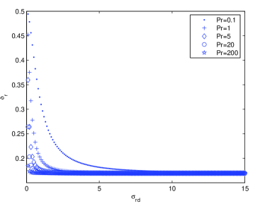
Figure 1: $\delta_{r}$ vs. $\sigma_{rd}$ for different values of $P_{r}$ when $m=50$.

In certain cases, source and relay are subject to a total power constraint. Here, we introduce the power allocation coefficient $\theta$, and total power constraint $P$. $P_{s}$ and $P_{r}$ have the following relations: $P_{s}=\theta P$, $P_{r}=(1-\theta)P$, and $P_{s}+P_{r}=P$. Next, we investigate how different values of $\theta$, and hence different power allocation strategies, affect the achievable rates. An analytical result for $\theta$ that maximizes the achievable rates is difficult to obtain. Therefore, we resort to numerical analysis. First, we consider the AF. The parameters we choose are $P=100,N_{0}=1,\delta_{s}=0.1,\delta_{r}=0.1$. Fig.2 plots the capacity lower bound (31) as a function of $\theta$ for different channel conditions, i.e., different values of $\sigma_{sr},\sigma_{rd},\text{ and }\sigma_{sd}$. We observe that the best performance is achieved when $\theta\approx 0.6$ and $\sigma_{sd}=1,\sigma_{sr}=4,\sigma_{rd}=4$ which indicates that both source-relay and relay-destination channels are favorable. When $\sigma_{sd}=1,\sigma_{sr}=2,\sigma_{rd}=1$, and hence the relay-destination and source-relay channels are not much better than the source-destination channel, the optimal value of $\theta$ is close to 1 and there is only little to be gained with cooperation.

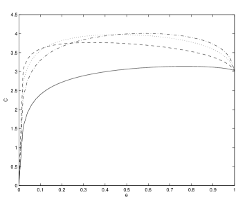
Figure 2: AF achievable rate vs. $\theta$. $P=100$. (1) the dashed line $\sigma_{sd}=1,\sigma_{sr}=10,\sigma_{rd}=2$; (2) the dotted line $\sigma_{sd}=1,\sigma_{sr}=6,\sigma_{rd}=3$; (3) the dashdot line $\sigma_{sd}=1,\sigma_{sr}=4,\sigma_{rd}=4$;(4) the solid line $\sigma_{sd}=1,\sigma_{sr}=2,\sigma_{rd}=1$

.

Figs. 3 and 4 plot the DF achievable rates as a function of $\theta$ with the same parameters as in the AF case. Hence, the total power is $P=100$. It is seen that paralel coding achieves a better performance compared to that of repetition coding. In parallel coding DF, we observe that unless $\sigma_{sr}$ is high and hence the source-relay channel is strong, the optimal value of $\theta$ is close to 1 and relay is allocated small power.

We consider in this paper that there is a cost associated with cooperation. This cost is the power and time dedicated to learn relay-destination channel. This cost is more pronounced in the presence of a low total power constraint. Figs. 5, 6, and 7 plot the achievable rates when $P=1$. We can see that DF have a better performance than AF at low power levels. Generally, cooperation gives more gains in the low power regime. However, as indicated by the solid-lined curves, if the quality of the source-relay and relay-destination channels is comparable to that of the source-destination channel, there is little or no gain through cooperation.

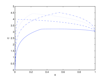
Figure 3: Repetition coding DF rate vs. $\theta$. $P=100$. (1) the dashed line $\sigma_{sd}=1,\sigma_{sr}=10,\sigma_{rd}=2$; (2) the dotted line $\sigma_{sd}=1,\sigma_{sr}=6,\sigma_{rd}=3$; (3) the dashdot line $\sigma_{sd}=1,\sigma_{sr}=4,\sigma_{rd}=4$; (4) the solid line $\sigma_{sd}=1,\sigma_{sr}=2,\sigma_{rd}=1$.

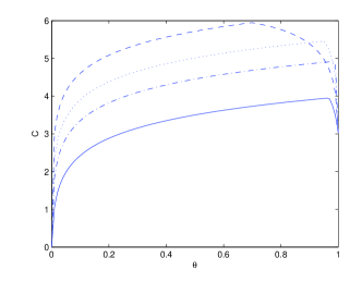
Figure 4: Parallel coding DF rate vs. $\theta$. $P=100$. From the top to bottom, the four curves correspond to (1) $\sigma_{sd}=1,\sigma_{sr}=10,\sigma_{rd}=2$ ; (2) $\sigma_{sd}=1,\sigma_{sr}=6,\sigma_{rd}=3$; (3) $\sigma_{sd}=1,\sigma_{sr}=4,\sigma_{rd}=4$; (4) $\sigma_{sd}=1,\sigma_{sr}=2,\sigma_{rd}=1$.

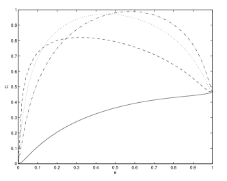
Figure 5: AF achievable rate vs. $\theta$. $P=1$. 1) the dashed line $\sigma_{sd}=1,\sigma_{sr}=10,\sigma_{rd}=2$; (2) the dotted line $\sigma_{sd}=1,\sigma_{sr}=6,\sigma_{rd}=3$; (3)the dashdot line $\sigma_{sd}=1,\sigma_{sr}=4,\sigma_{rd}=4$;(4) the solid line $\sigma_{sd}=1,\sigma_{sr}=2,\sigma_{rd}=1$

.

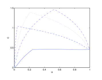
Figure 6: Repetition coding DF rate vs. $\theta$. $P=1$. (1) the dashed line $\sigma_{sd}=1,\sigma_{sr}=10,\sigma_{rd}=2$; (2) the dotted line $\sigma_{sd}=1,\sigma_{sr}=6,\sigma_{rd}=3$; (3) the dashdot line $\sigma_{sd}=1,\sigma_{sr}=4,\sigma_{rd}=4$; (4) the solid line $\sigma_{sd}=1,\sigma_{sr}=2,\sigma_{rd}=1$;

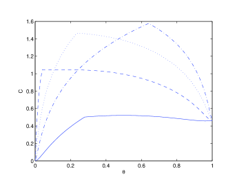
Figure 7: Parallel coding DF rate vs. $\theta$. $P=1$.(1) the dashed line $\sigma_{sd}=1,\sigma_{sr}=10,\sigma_{rd}=2$; (2) the dotted line $\sigma_{sd}=1,\sigma_{sr}=6,\sigma_{rd}=3$; (3) the dashdot line $\sigma_{sd}=1,\sigma_{sr}=4,\sigma_{rd}=4$;(4) the solid line $\sigma_{sd}=1,\sigma_{sr}=2,\sigma_{rd}=1$.

References

- [1] J.N. Laneman, D.N.C. Tse, G.W. Wornel “Cooperative diversity in wireless networks: Efficient protocols and outage behavior,” IEEE Trans. Inform. Theory, vol.50,pp.3062-3080. Dec.2004
- [2] J. N. Laneman, “Cooperation in wireless networks: Principles and applications,” Springer, 2006, ch.1 Cooperative Diversity: Models, Algorithms, and Architectures
- [3] R.U. Nabar, H. Bolcskei, F.W. Kneubuhler, “Fading Relay Channels:Performance Limits and Space-Time Signal Design,” IEEE J.Select. Areas Commun vol.22,NO.6 pp1099-1109. Aug.2004
- [4] A. Host-Madsen, “Capacity bounds for cooperative diversity,” IEEE Trans. Inform. Theory, vol. 52, no. 4, pp. 1522 1544, Apr. 2006.
- [5] G. Kramer, M. Gastpar, and P. Gupta, “Cooperative strategies and capacity theorems for relay networks,” IEEE Trans. Inform. Theory, vol. 51, no. 9, pp. 3037 3063, Sept. 2005.
- [6] Y. Liang and V. V. Veeravalli, “Gaussian orthogonal relay channels: Optimal resource allocation and capacity,” IEEE Trans. Inform. Theory, vol. 51, no. 9, pp. 3284 3289, Sept. 2005.
- [7] P. Mitran, H. Ochiai, and V. Tarokh, “Space-time diversity enhancements using collaborative communications,” IEEE Trans. Inform. Theory, vol. 51, no. 6, pp. 2041 2057, June 2005.
- [8] Y. Yao, X. Cai, and G. B. Giannakis, “On energy efficiency and optimum resource allocation of relay tranmissions in the low-power regime,” IEEE Trans. Wireless Commun., vol. 4, no. 6, pp. 2917 2927, Nov. 2005.
- [9] B.Wang, J.Zhang, L.Zheng, “Achievable rates and scaling laws of power-constrained wireless sensory relay networks” IEEE Tran. Inform. Theory, vol.52,NO.9 Sep.2006
- [10] M. Medard “The effect upon channel capacity in wireless communication of perfect and imperfect knowledge of the channel,” IEEE Trans. Inform. Theory, vol.46,pp.933-946,May.2000
- [11] B. Hassibi, B. M. Hochwald, ”How much training is needed in multiple-antenna wireless link?,”IEEE Trans. Inform. Theory, vol.49,pp.951-964,April.2003
- [12] M.C. Gursoy, “An energy efficiency perspective on training for fading channels,” to appear in the Proceedings of the IEEE ISIT 2007.