On the Kinetostatic Optimization of Revolute-Coupled Planar Manipulators

Abstract

Proposed in this paper is a kinetostatic performance index for the optimum dimensioning of planar manipulators of the serial type. The index is based on the concept of distance of the underlying Jacobian matrix to a given isotropic matrix that is used as a reference model for purposes of performance evaluation. Applications of the index fall in the realm of design, but control applications are outlined. The paper focuses on planar manipulators, the basic concepts being currently extended to their three-dimensional counterparts.

url]www.irccyn.ec-nantes.fr

url]www.cim.mcgill.ca

1 Introduction

Various performance indices have been devised to asses the kinetostatic performance of serial manipulators. Among these, the concepts of service angle [1], dexterous workspace [2] and manipulability [3] are worth mentioning. All these different concepts allow the definition of the kinetostatic performance of a manipulator from correspondingly different viewpoints. However, with the exception of Yoshikawa’s manipulability index [3], none of these considers the invertibility of the Jacobian matrix. A dimensionless quality index was recently introduced by Lee [4] based on the ratio of the Jacobian determinant to its maximum absolute value, as applicable to parallel manipulators. This index does not take into account the location of the operation point in the end-effector, for the Jacobian determinant is independent of this location. The proof of the foregoing fact is available in [5], as pertaining to serial manipulators, its extension to their parallel counterparts being straightforward. The condition number of a given matrix is well known to provide a measure of invertibility of the matrix [6]. It is thus natural that this concept found its way in this context. Indeed, the condition number of the Jacobian matrix was proposed by Salisbury [7] as a figure of merit to minimize when designing manipulators for maximum accuracy. In fact, the condition number gives, for a square matrix, a measure of the relative roundoff-error amplification of the computed results [6] with respect to the data roundoff error. As is well known, however, the dimensional inhomogeneity of the entries of the Jacobian matrix prevents the straightforward application of the condition number as a measure of Jacobian invertibility. The characteristic length was introduced in [8] to cope with the above-mentioned inhomogeneity. Apparently, nevertheless, this concept has found strong opposition within some circles, mainly because of the lack of a direct geometric interpretation of the concept. It is the aim of this paper to shed more light in this debate, while proposing a novel performance index that lends itself to a straightforward manipulation and leads to sound geometric relations. Briefly stated, the performance index proposed here is based on the concept of distance in the space of $m\times n$ matrices, which is based, in turn, on the concept of inner product of this space. The performance index underlying this paper thus measures the distance of a given Jacobian matrix from an isotropic matrix of the same gestalt. With the purpose of rendering the Jacobian matrix dimensionally homogeneous, we resort to the concept of posture-dependent conditioning length. Thus, given an arbitrary serial manipulator in an arbitrary posture, it is possible to define a unique length that renders this matrix dimensionally homogeneous and of minimum distance to isotropy. The characteristic length of the manipulator is then defined as the conditioning length corresponding to the posture that renders the above-mentioned distance a minimum over all possible manipulator postures. This paper is devoted to planar manipulators, the concepts being currently extended to spatial ones.

2 Algebraic Background

Given two arbitrary $m\times n$ matrices A and B of real entries, their inner product, represented by $({\bf{A}},\,{\bf{B}})$, is defined as

$$({\bf{A}},\,{\bf{B}})\equiv{\rm tr}({\bf{A}}{\bf{W}}{\bf{B}}^{T})$$ (1)

where W is a positive-definite $n\times n$ weighting matrix that is introduced to allow for suitable normalization. The entries of W need not be dimensionally homogeneous, and, in fact, they should not if A and B are not. However, the product ${\bf{A}}{\bf{W}}{\bf{B}}^{T}$ must be dimensionally homogeneous; else, its trace is meaningless. The norm of the space of $m\times n$ matrices induced by the above inner product is thus the Frobenius norm, namely,

$$\|{\bf{A}}\|^{2}={\rm tr}({\bf{A}}{\bf{W}}{\bf{A}}^{T})$$ (2a)

Moreover, we shall be handling only nondimensional matrix entries, and hence, we choose W non-dimensional as well, and so as to yield a value of unity for the norm of the $$n\times n$$ identity matrix 1. Hence,

$${\bf{W}}\equiv\frac{1}{n}{\bf{1}}$$ (2b)

The foregoing inner product is thus expressed as

$$({\bf{A}},\,{\bf{B}})\equiv\frac{1}{n}{\rm tr}({\bf{A}}{\bf{B}}^{T})$$ (2c)

Henceforth we shall use only the Frobenius norm; for brevity, this will be simply referred to as the norm of a given matrix.

When comparing two dimensionless $m\times n$ matrices A and B, we can define their distance $d({\bf{A}},\,{\bf{B}})$ as the Frobenius norm of their difference, namely,

$$d({\bf{A}},\,{\bf{B}})\equiv\|{\bf{A}}-{\bf{B}}\|$$ (3a)

i.e.,

$$d({\bf{A}},\,{\bf{B}})\equiv\sqrt{\frac{1}{n}{\rm tr}[({\bf{A}}-{\bf{B}})({\bf{A}}-{\bf{B}})^{T}]}$$ (3b)

An $m\times n$ isotropic matrix, with $m<n$, is one with a singular value $\sigma>0$ of multiplicity $m$, and hence, if the $m\times n$ matrix C is isotropic, then

$${\bf{C}}{\bf{C}}^{T}=\sigma^{2}{\bf{1}}$$ (4)

where 1 is the $m\times m$ identity matrix. Note that the generalized inverse of C can be computed without roundoff-error, for it is proportional to ${\bf{C}}^{T}$, namely,

$$({\bf{C}}{\bf{C}}^{T})^{-1}{\bf{C}}^{T}=\frac{1}{\sigma^{2}}{\bf{C}}^{T}$$ (5)

Furthermore, the condition number $\kappa({\bf{A}})$ of a square matrix A is defined [6] as

$$\kappa({\bf{A}})=\|{\bf{A}}\|\|{\bf{A}}^{-1}\|$$ (6)

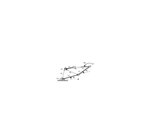
Figure 1: Planar $n$-revolute manipulator

where any norm can be used. For purposes of the paper, we shall use the Frobenius norm for matrices and the Euclidian norm for vectors. Henceforth we assume, moreover, a planar $n$-revolute manipulator, as depicted in Fig. 1, with Jacobian matrix J given by Angeles [5]

$${\bf{J}}=\left[\begin{array}[]{cccc}1&1&\cdots&1\\ {\bf{E}}{\bf{r}}_{1}&{\bf{E}}{\bf{r}}_{2}&\cdots&{\bf{E}}{\bf{r}}_{n}\end{array}\right]$$ (9)

where ${\bf{r}}_{i}$ is the vector directed from the center of the $i$th revolute to the operation point $P$ of the end-effector, while matrix ${\bf{E}}$ is defined as

$${\bf{E}}=\left[\begin{array}[]{cc}0&-1\\ 1&0\end{array}\right]$$ (12)

i.e., E represents a counterclockwise rotation of $90^{\circ}$. It will prove convenient to partition J in the form

$${\bf{J}}=\left[\begin{array}[]{c}{\bf{A}}\\ {\bf{B}}\end{array}\right]$$ (15)

with A and B defined as

$${\bf{A}}=\left[\begin{array}[]{cccc}1&1&\cdots&1\end{array}\right]{\rm~{}~{}~{}~{}and~{}~{}~{}~{}}{\bf{B}}=\left[\begin{array}[]{cccc}{\bf{E}}{\bf{r}}_{1}&{\bf{E}}{\bf{r}}_{2}&\cdots&{\bf{E}}{\bf{r}}_{n}\end{array}\right]$$ (18)

Therefore, while the entries of A are dimensionless, those of B have units of length. Thus, the sole singular value of A, i.e. the nonnegative square root of the scalar of ${\bf{A}}{\bf{A}}^{T}$, is $\sqrt{n}$, and hence, dimensionless, and pertains to the mapping from joint-rates into end-effector angular velocity. The singular values of B, which are the nonnegative square roots of the eigenvalues of ${\bf{B}}{\bf{B}}^{T}$, have units of length, and account for the mapping from joint-rates into operation-point velocity. It is thus apparent that the singular values of ${\bf{J}}$ have different dimensions and hence, it is impossible to compute $\kappa({\bf{J}})$ as in eq.(6), for the norm of ${\bf{J}}$, as defined in eqs.(2a & b), is meaningless. The normalization of the Jacobian for purposes of rendering it dimensionless has been judged to be dependent on the normalizing length [9]. As a means to avoid the arbitrariness of the choice of that normalizing length, the characteristic length $L$ was introduced in [10]. Since the calculation of $L$ is based on the minimization of an objective function that is elusive to a straightforward geometric interpretation, namely, the condition number of the normalized Jacobian, the characteristic length has been found cumbersome to use in manipulator design. We introduce below the concept of conditioning length to render the Jacobian matrix dimensionless, which will allow us to define the characteristic length using a geometric approach. In the sequel, we will need the partial derivative of the trace of a square matrix N with respect to a scalar argument $x$ of N. The said derivative is readily obtained as

$$\frac{\partial}{\partial x}{\rm tr}({\bf{N}})={\rm tr}\left(\frac{\partial{\bf{N}}}{\partial x}\right)$$ (19a)

Moreover, in some instances, we will need the partial derivative of a scalar function $$f x$$ of the matrix argument N with respect to the scalar , which is, in turn, an argument of N. In this case, the desired partial derivative is obtained by application of the chain rule:

$$\frac{\partial f}{\partial x}={\rm tr}\left(\frac{\partial f}{\partial{\bf{N}}}\frac{\partial{\bf{N}}^{T}}{\partial x}\right)$$ (19b)

In particular, when $$f({\bf{N}}) k N_{k} x$$ is the th moment of N with respect to , defined as

$$N_{k}\equiv{\rm tr}({\bf{N}}^{k})$$ (19c)

the partial derivative of $$N_{k} x$$ with respect to is given by

$$\frac{\partial N_{k}}{\partial x}=k{\rm tr}\left({\bf{N}}^{k-1}\frac{\partial{\bf{N}}^{T}}{\partial x}\right)$$ (19d)

Furthermore, we recall that the trace of any square matrix N equals that of its transpose, i.e.,

$${\rm tr}({\bf{N}}^{T})={\rm tr}({\bf{N}})$$ (20a)

and, finally, the trace of a product of various matrices compatible under multiplication does not change under a cyclic permutation of the factors, i.e., if A, B, and C are three matrices whose product $${\bf{A}}{\bf{B}}{\bf{C}}$$ is possible and square, then tr(ABC) =tr(BCA)= tr(CAB)

3 Isotropic Sets of Points

Consider the set ${\mathcal{S}}\equiv\{\,P_{k}\,\}_{1}^{n}$ of $n$ points in the plane, of position vectors $\{\,{\bf{p}}_{k}\,\}_{1}^{n}$, and centroid $C$, of position vector c, i.e.,

$${\bf{c}}\equiv\frac{1}{n}\sum_{1}^{n}{\bf{p}}_{k}$$ (21)

The summation appearing in the right-hand side of the above expression is known as the first moment of $\mathcal{S}$ with respect to the origin $O$ from which the position vectors stem. The second moment of $\mathcal{S}$ with respect to $C$ is defined as a tensor M, namely,

$${\bf{M}}\equiv\sum_{1}^{n}({\bf{p}}_{k}-{\bf{c}})({\bf{p}}_{k}-{\bf{c}})^{T}$$ (22)

It is now apparent that the root-mean square value of the distances $\{\,d_{k}\,\}_{1}^{n}$ of $\mathcal{S}$, $d_{\rm rms}$, to the centroid is directly related to the trace of M, namely,

$$d_{\rm rms}\equiv\sqrt{\frac{1}{n}\sum_{1}^{n}({\bf{p}}_{k}-{\bf{c}})^{T}({\bf{p}}_{k}-{\bf{c}})}\equiv\sqrt{\frac{1}{n}{\rm tr}({\bf{M}})}$$ (23)

Further, the moment of inertia I of $\mathcal{S}$ with respect to the centroid is defined as that of a set of unit masses located at the points of $\mathcal{S}$, i.e.,

$${\bf{I}}\equiv\sum_{1}^{n}[\,\|{\bf{p}}_{k}-{\bf{c}}\|^{2}{\bf{1}}-({\bf{p}}_{k}-{\bf{c}})({\bf{p}}_{k}-{\bf{c}})^{T}\,]$$ (24a)

in which 1 is the $$2\times 2$$ identity matrix. Hence, in light of definitions (22) and (23),

$${\bf{I}}={\rm tr}({\bf{M}}){\bf{1}}-{\bf{M}}$$ (24b)

We shall refer to I as the geometric moment of inertia of $\mathcal{S}$ about its centroid. It is now apparent that I is composed of two parts, an isotropic matrix of norm ${\rm tr}({\bf{M}})$ and the second moment of $\mathcal{S}$ with the sign reversed. Moreover, the moment of inertia I can be expressed in a form that is more explicitly dependent upon the set $\{\,{\bf{p}}_{k}-{\bf{c}}\,\}_{1}^{n}$, if we recall the concept of cross-product matrix [5]. Briefly stated, for any three-dimensional vector v, we define the cross-product matrix ${\bf{P}}_{k}$ of $({\bf{p}}_{k}-{\bf{c}})$, or of any other three-dimensional vector for that matter, as

$${\bf{P}}_{k}\equiv\frac{\partial[({\bf{p}}_{k}-{\bf{c}})\times{\bf{v}}]}{\partial{\bf{v}}}$$ (25a)

Further, we recall the identity [5]

$${\bf{P}}_{k}^{2}\equiv-\|{\bf{p}}_{k}-{\bf{c}}\|^{2}{\bf{1}}+({\bf{p}}_{k}-{\bf{c}})({\bf{p}}_{k}-{\bf{c}})^{T}$$ (25b)

It is now apparent that the moment of inertia of $\mathcal{S}$ takes the simple form

$${\bf{I}}=-\sum_{1}^{n}{\bf{P}}_{k}^{2}$$ (26)

We thus have

Definition 1 (Isotropic Set)

The set $\mathcal{S}$ is said to be isotropic if its second-moment tensor with respect to its centroid is isotropic.

As a consequence, we have

Lemma 1

The geometric moment of inertia of an isotropic set of points about its centroid is isotropic.

3.1 Geometric Properties of Isotropic Sets of Points

We describe below some properties of isotropic sets of points that will help us better visualize the results that follow.

3.1.1 Union of Two Isotropic Sets of Points

Consider two isotropic sets of points in the plane, ${\mathcal{S}}_{1}=\{\,P_{k}\,\}_{1}^{n}$ and ${\mathcal{S}}_{2}=\{\,P_{k}\,\}_{n+1}^{n+m}$. If the centroid $C$ of the position vector ${\bf{c}}$ of ${\mathcal{S}}_{1}$ coincides with that of ${\mathcal{S}}_{2}$, i.e. if,

$${\bf{c}}\equiv\frac{1}{n}\sum_{1}^{n}{\bf{p}}_{k}\equiv\frac{1}{m}\sum_{n+1}^{n+m}{\bf{p}}_{k}$$ (27)

then, the set ${\mathcal{S}}={\mathcal{S}}_{1}\cup{\mathcal{S}}_{2}$ is isotropic.

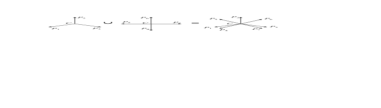
Figure 2: Union of two isotropic sets of points

For example, let ${\mathcal{S}}_{1}$ be a set of three isotropic points and ${\mathcal{S}}_{2}$ a set of four isotropic points, as displayed in Fig. 2, i.e.,

$${\mathcal{S}}_{1} = \left\{\left[\begin{array}[]{c}-\sqrt{6}/2\\ -\sqrt{2}/2\end{array}\right],\left[\begin{array}[]{c}~{}\sqrt{6}/2\\ -\sqrt{2}/2\end{array}\right],\left[\begin{array}[]{c}0\\ \sqrt{2}\end{array}\right]\right\}$$ (28g)

$${\mathcal{S}}_{2} = \left\{\left[\begin{array}[]{c}0\\ -\sqrt{2}\end{array}\right],\left[\begin{array}[]{c}-\sqrt{2}\\ 0\end{array}\right],\left[\begin{array}[]{c}0\\ \sqrt{2}\end{array}\right],\left[\begin{array}[]{c}\sqrt{2}\\ 0\end{array}\right]\right\}$$ (28p)

where the centroid $$C \mathcal{S} \mathcal{C}$$ is the origin. The second moment of with respect to is isotropic, namely,

$${\bf{M}}\equiv\sum_{1}^{3+4}({\bf{p}}_{k}-{\bf{c}})({\bf{p}}_{k}-{\bf{c}})^{T}=\left[\begin{array}[]{cc}7&0\\ 0&7\end{array}\right]=(7){\bf{1}}$$ (28q)

where 1 denotes the $2\times 2$ identity matrix. Furthermore, the geometric moment of inertia of $\mathcal{S}$ is

$${\bf{1}}=(14){\bf{1}}-(7){\bf{1}}=(7){\bf{1}}$$

Lemma 2

The union of two isotropic sets of points sharing the same centroid is also isotropic.

3.1.2 Rotation of an Isotropic Set of Points

Let ${\bf{R}}$ denote a rotation matrix in the plane through an angle $\alpha$ and ${\mathcal{S}}=\{\,P_{k}\,\}_{1}^{n}$ a set of isotropic points. A new set of points ${\mathcal{S}^{\prime}}=\{\,P^{\prime}_{k}\,\}_{1}^{n}$ is defined upon rotating ${\mathcal{S}}$ through an angle $\alpha$ about $C$ as a rigid body. The second moment of $\mathcal{S}^{\prime}$ with respect to $C$ is shown below to be isotropic as well. Indeed, letting this moment be ${\bf{M}}^{\prime}$, we have

$${\bf{M}}^{\prime}\equiv\sum_{1}^{n}({\bf{p}}_{k}^{\prime}-{\bf{c}}^{\prime})({\bf{p}}_{k}^{\prime}-{\bf{c}}^{\prime})^{T}$$

where, by definition,

$${\bf{p}}_{k}^{\prime}-{\bf{c}}^{\prime}={\bf{R}}({\bf{p}}_{k}-{\bf{c}})$$

Thus,

$${\bf{M}}^{\prime}\equiv\sum_{1}^{n}{\bf{R}}({\bf{p}}_{k}-{\bf{c}})({\bf{p}}_{k}-{\bf{c}})^{T}{\bf{R}}^{T}={\bf{R}}[\,\sum_{1}^{n}({\bf{p}}_{k}-{\bf{c}})({\bf{p}}_{k}-{\bf{c}})^{T}]{\bf{R}}^{T}$$

But the summation in brackets is the second moment M of the set $\mathcal{S}$, which is, by assumption, isotropic, and hence, takes the form

$${\bf{M}}=\sum_{1}^{n}({\bf{p}}_{k}-{\bf{c}})({\bf{p}}_{k}-{\bf{c}})^{T}=\sigma^{2}{\bf{1}}$$

for a real number $\sigma>0$ and 1 denoting the $2\times 2$ identity matrix. Hence,

$${\bf{M}}^{\prime}=\sigma^{2}{\bf{R}}{\bf{R}}^{T}=\sigma^{2}{\bf{1}}$$

thereby proving that the rotated set is isotropic as well. We thus have

Lemma 3

The rotation of an isotropic set of points as a rigid body with respect to its centroid is also isotropic.

The counterclockwise rotation of an isotropic set of three points, $\mathcal{S}$, through an angle of $60^{\circ}$ and the union of the original set and its rotated counterpart are depicted in Fig. 3. Note that the union of the two sets is isotropic as well.

3.1.3 Trivial Isotropic Set of Points

An isotropic set of points can be defined by the union or rotation, or a combination of both, of isotropic sets. The simplest set of isotropic points is the set of vertices of a regular polygon. We thus have

Definition 2 (Trivial isotropic set)

A set of $n$ points ${\mathcal{S}}$ is called trivial if it is the set of vertices of a regular polygon with $n$ vertices.

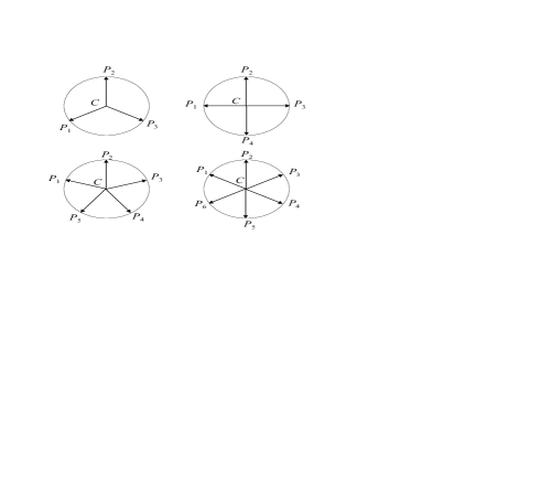
Figure 4: Trivial isotropic sets for $n=3,\cdots,6$

Trivial isotropic sets, ${\mathcal{S}}=\{\,P_{k}\,\}_{1}^{n}$ are depicted in Fig. 4, for $n=3,\cdots,6$.

Also note that

Lemma 4

A trivial isotropic set $\mathcal{S}$ remains isotropic under every reflection about an axis passing through the centroid $C$.

4 An Outline of Kinematic Chains

The connection between sets of points and planar manipulators of the serial type is the concept of simple kinematic chain. For completeness, we recall here some basic definitions pertaining to this concept.

4.1 Simple Kinematic Chains

The kinematics of manipulators is based on the concept of kinematic chain. A kinematic chain is a set of rigid bodies, also called links, coupled by kinematic pairs. In the case of planar chains, two lower kinematic pairs are possible, the revolute, allowing pure rotation of the two coupled links, and the prismatic pair, allowing a pure relative translation, along one direction, of the same links. For the purpose of this paper, we study only revolute pairs, but prismatic pairs are also common in manipulators.

Definition 3 (Simple kinematic chain)

A kinematic chain is said to be simple if each and every one of its links is coupled to at most two other links.

A simple kinematic chain can be open or closed; in studying serial manipulators we are interested in the former. In such a chain, we distinguish exactly two links, the terminal ones, coupled to only one other link. These links are thus said to be simple, all other links being binary. In the context of manipulator kinematics, one terminal link is arbitrarily designated as fixed, the other terminal link being the end-effector (EE), which is the one executing the task at hand. The task is defined, in turn, as a sequence of poses—positions and orientations—of the EE, the position being given at a specific point $P$ of the EE that we term the operation point.

4.2 Isotropic Kinematic Chains

To every set $\mathcal{S}$ of $n$ points it is possible to associate a number of kinematic chains. To do this, we number the points from 1 to $n$, thereby defining $n-1$ links, the $i$th link carrying joints $i$ and $i+1$. Links are thus correspondingly numbered from 1 to $n$, the $n$th link, or EE, carrying joint $n$ on its proximal (to the base) end and the operation point $P$ on its distal end. Furthermore, we define an additional link, the base, which is numbered as 0.

It is now apparent that, since we can number a given set $\mathcal{S}$ of $n$ points in $n!$ possible ways, we can associate $n!$ kinematic chains to the above set $\mathcal{S}$ of $n$ points. Clearly, these chains are, in general, different, for the lengths of their links are different as well. Nevertheless, some pairs of identical chains in the foregoing set are possible.

Definition 4 (Isotropic kinematic chain)

If the foregoing set $\mathcal{S}$ of $n$ points is isotropic, and the operation point $P$ is defined as the centroid of $\mathcal{S}$, then any kinematic chain stemming from $\mathcal{S}$ is isotropic.

5 The Posture-Dependent Conditioning Length of Planar n-Revolute Manipulators

Under the assumption that the manipulator finds itself at a posture $\mathcal{P}$ that is given by its set of joint angles, $\{\,\theta_{k}\,\}_{1}^{n}$, we start by dividing the last $n$ rows of the Jacobian by a length $l_{\mathcal{P}}$, as yet to be determined. This length will be found so as to minimize the distance of the normalized Jacobian to a corresponding isotropic matrix K, subscript $\mathcal{P}$ reminding us that, as the manipulator changes its posture, so does the length $l_{\mathcal{P}}$. This length will be termed the conditioning length of the manipulator at $\mathcal{P}$.

5.1 A Dimensionally-Homogeneous Jacobian Matrix

In order to distinguish the original Jacobian matrix from its dimensionally-homogeneous counterpart, we shall denote the latter by $\overline{{\bf{J}}}$, i.e.,

$$\overline{{\bf{J}}}=\left[\begin{array}[]{cccc}1&1&\cdots&1\\ (1/l_{\mathcal{P}})~{}{\bf{E}}{\bf{r}}_{1}&(1/l_{\mathcal{P}})~{}{\bf{E}}{\bf{r}}_{2}&\cdots&(1/l_{\mathcal{P}})~{}{\bf{E}}{\bf{r}}_{n}\end{array}\right]$$ (31)

Now the conditioning length will be defined via the minimization of the distance of the dimensionally-homogeneous Jacobian matrix $\overline{{\bf{J}}}$ of an $n$-revolute manipulator to an isotropic $3\times n$ model matrix K whose entries are dimensionless and has the same gestalt as any $3\times n$ Jacobian matrix. To this end, we define an isotropic set ${\mathcal{K}}=\{\,K_{i}\,\}_{1}^{n}$ of $n$ points in a dimensionless plane, of position vectors $\{\,{\bf{k}}_{i}\,\}_{1}^{n}$, which thus yields the dimensionless matrix

$${\bf{K}}=\left[\begin{array}[]{cccc}1&1&\cdots&1\\ {\bf{E}}{\bf{k}}_{1}&{\bf{E}}{\bf{k}}_{2}&\cdots&{\bf{E}}{\bf{k}}_{n}\end{array}\right]$$ (32)

Further, we compute the product ${\bf{K}}{\bf{K}}^{T}$:

$${\bf{K}}{\bf{K}}^{T}=\left[\begin{array}[]{cc}n&\sum_{1}^{n}{\bf{k}}_{i}^{T}{\bf{E}}^{T}\\ \sum_{1}^{n}{\bf{E}}{\bf{k}}_{i}&\sum_{1}^{n}{\bf{E}}{\bf{k}}_{i}{\bf{k}}_{i}^{T}{\bf{E}}^{T}\end{array}\right]$$ (35)

Upon expansion of the summations occurring in the above matrix, we have

$$\sum_{1}^{n}{\bf{k}}_{i}^{T}{\bf{E}}^{T} = (\sum_{1}^{n}{\bf{E}}{\bf{k}}_{i})^{T}={\bf{E}}(\sum_{1}^{n}{\bf{k}}_{i})^{T}$$ (36a)

$$\sum_{1}^{n}{\bf{E}}{\bf{k}}_{i}{\bf{k}}_{i}^{T}{\bf{E}}^{T} = {\bf{E}}(\sum_{1}^{n}{\bf{k}}_{i}{\bf{k}}_{i}^{T}){\bf{E}}^{T}$$ (36b)

Now, by virtue of the assumed isotropy of $\mathcal{K}$, the terms in parentheses in the foregoing expressions become

$$\sum_{1}^{n}{\bf{k}}_{i} = {\bf{0}}$$

$$\sum_{1}^{n}{\bf{k}}_{i}{\bf{k}}_{i}^{T} = k^{2}{\bf{1}}_{2\times 2}$$

where the factor $k^{2}$ is as yet to be determined and ${\bf{1}}_{2\times 2}$ denotes the $2\times 2$ identity matrix. Hence, the product ${\bf{K}}{\bf{K}}^{T}$ takes the form

$${\bf{K}}{\bf{K}}^{T}=\left[\begin{array}[]{cc}n&{\bf{0}}^{T}\\ {\bf{0}}&k^{2}{\bf{1}}_{2\times 2}\end{array}\right]$$ (37)

Now, in order to determine $k^{2}$, we recall that matrix K is isotropic, and hence that the product ${\bf{K}}{\bf{K}}^{T}$ has a triple eigenvalue. It is now apparent that the triple eigenvalue of the said product must be $n$, which means that

$$k^{2}=n$$ (38)

and hence,

$$\sum_{1}^{n}{\bf{k}}_{i}{\bf{k}}_{i}^{T}=(n){\bf{1}}_{2\times 2}$$

5.2 Example 1: A Three-DOF Planar Manipulator

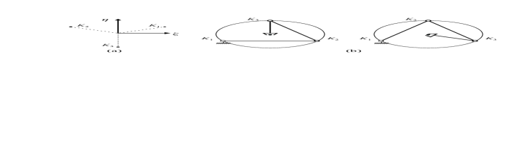
Figure 5: Two isotropic manipulator postures stemming from the same isotropic set upon a relabelling of its points

Shown in Fig. 5a is an isotropic set $\mathcal{K}$ of three points, of position vectors $\{\,{\bf{k}}_{i}\,\}_{1}^{n}$, in a nondimensional plane. The position vectors are given by

$${\bf{k}}_{1}=\frac{1}{2}\left[\begin{array}[]{c}\sqrt{6}\\ \sqrt{2}\end{array}\right]{~{}\rm,~{}}{\bf{k}}_{2}=\frac{1}{2}\left[\begin{array}[]{c}-\sqrt{6}\\ ~{}\sqrt{2}\end{array}\right]{~{}\rm,~{}}{\bf{k}}_{3}=\left[\begin{array}[]{c}0\\ -\sqrt{2}\end{array}\right]$$ (39a)

Hence, the corresponding model matrix is

$${\bf{K}}=\left[\begin{array}[]{ccc}1&1&1\\ -\sqrt{2}/2&-\sqrt{2}/2&~{}\sqrt{2}\\ ~{}\sqrt{6}/2&-\sqrt{6}/2&0\end{array}\right]$$ (39b)

which can readily be proven to be isotropic, with a triple singular value of $k=\sqrt{3}$. When the order of the three vectors is changed, the isotropic condition is obviously preserved, for such a reordering amounts to nothing but a relabelling of the points of $\mathcal{K}$. Also note that two isotropic matrices ${\bf{K}}$ are associated with two symmetric postures, as displayed in Fig. 5b

5.3 Example 2: A Four-DOF Redundant Planar Manipulator

An isotropic set $\mathcal{K}$ of four points, $\{\,K_{i}\,\}_{1}^{4}$, is defined in a nondimensional plane, with position vectors ${\bf{k}}_{i}$ given below:

$${\bf{k}}_{1}=\left[\begin{array}[]{c}\sqrt{2}\\ \sqrt{2}\end{array}\right]{~{}\rm,~{}}{\bf{k}}_{2}=\left[\begin{array}[]{c}-\sqrt{2}\\ ~{}\sqrt{2}\end{array}\right]{~{}\rm,~{}}{\bf{k}}_{3}=\left[\begin{array}[]{c}-\sqrt{2}\\ -\sqrt{2}\end{array}\right]{~{}\rm,~{}}{\bf{k}}_{4}=\left[\begin{array}[]{c}~{}\sqrt{2}\\ -\sqrt{2}\end{array}\right]$$ (40a)

which thus lead to

$${\bf{K}}=\left[\begin{array}[]{cccc}1&1&1&1\\ -\sqrt{2}&-\sqrt{2}&\sqrt{2}&\sqrt{2}\\ \sqrt{2}&-\sqrt{2}&-\sqrt{2}&\sqrt{2}\end{array}\right]$$ (40b)

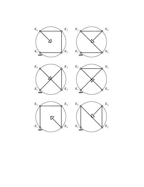
Figure 6: Six isotropic postures for the same isotropic set

We thus have $4!=24$ isotropic kinematic chains for a four-dof planar manipulator, but we represent only $6$ in Fig. 6 because the choice of the first point is immaterial, since this choice amounts to a rotation of the overall manipulator as a rigid body.

5.4 Computation of the Conditioning Length

We can now formulate a least-square problem aimed at finding the conditioning length $l_{\mathcal{P}}$ that renders the distance from $\overline{{\bf{J}}}$ to K a minimum. The task will be eased if we work rather with the reciprocal of $l_{\mathcal{P}}$, $\lambda\equiv 1/l_{\mathcal{P}}$, and hence,

$$z\equiv\frac{1}{2}\frac{1}{n}{\rm tr}[(\overline{{\bf{J}}}-{\bf{K}})(\overline{{\bf{J}}}-{\bf{K}})^{T}]\quad\rightarrow\quad\min_{\lambda}$$ (41)

Upon expansion,

$$z=\frac{1}{2}\frac{1}{n}{\rm tr}(\overline{{\bf{J}}}\overline{{\bf{J}}}^{T}-\overline{{\bf{J}}}{\bf{K}}^{T}-{\bf{K}}\overline{{\bf{J}}}^{T}+{\bf{K}}{\bf{K}}^{T})$$

Since the trace of a matrix equals that of its transpose, i.e.,

$${\rm tr}(\overline{{\bf{J}}}{\bf{K}}^{T})={\rm tr}({\bf{K}}\overline{{\bf{J}}}^{T})$$

the foregoing expression for $z$ reduces to

$$z\equiv\frac{1}{2}\frac{1}{n}{\rm tr}(\overline{{\bf{J}}}\overline{{\bf{J}}}^{T}-2{\bf{K}}\overline{{\bf{J}}}^{T}+{\bf{K}}{\bf{K}}^{T})$$ (42)

It is noteworthy that the above minimization problem is (a) quadratic in $\lambda$, for $\overline{{\bf{J}}}$ is linear in $\lambda$ and (b) unconstrained, which means that the problem accepts a unique solution. This solution can be found, additionally, in closed form. Indeed, the optimum value of $\lambda$ is readily obtained upon setting up the normality condition of the above problem, namely,

$$\frac{\partial z}{\partial\lambda}\equiv\frac{1}{2n}{\rm tr}\left(\frac{\partial(\overline{{\bf{J}}}~{}\overline{{\bf{J}}}^{T})}{\partial\lambda}\right)-\frac{1}{n}{\rm tr}\left({\bf{K}}\frac{\partial\overline{{\bf{J}}}^{T}}{\partial\lambda}\right)=0$$ (43)

where we have used the linearity property of the trace and the derivative operators. We calculate below the quantities involved:

$$\overline{{\bf{J}}}\overline{{\bf{J}}}^{T}=\left[\begin{array}[]{cc}n&\lambda\sum_{1}^{n}{\bf{r}}_{j}^{T}{\bf{E}}^{T}\\ \lambda\sum_{1}n3{\bf{E}}{\bf{r}}_{j}&\lambda^{2}\sum_{1}^{n}{\bf{E}}{\bf{r}}_{j}{\bf{r}}_{j}^{T}{\bf{E}}^{T}\end{array}\right]{\rm,}{\bf{K}}\overline{{\bf{J}}}^{T}=\left[\begin{array}[]{cc}n&\lambda\sum_{1}^{n}{\bf{r}}_{j}^{T}{\bf{E}}^{T}\\ \sum_{1}^{n}{\bf{E}}{\bf{k}}_{j}&\lambda\sum_{1}^{n}{\bf{E}}{\bf{k}}_{j}{\bf{r}}_{j}^{T}{\bf{E}}^{T}\end{array}\right]$$

Thus,

$$\frac{\partial(\overline{{\bf{J}}}\overline{{\bf{J}}}^{T})}{\partial\lambda}=\left[\begin{array}[]{cc}0&\sum_{1}^{n}{\bf{r}}_{j}^{T}{\bf{E}}^{T}\\ \sum_{1}^{n}{\bf{E}}{\bf{r}}_{j}&2\lambda\sum_{1}^{n}{\bf{E}}{\bf{r}}_{j}{\bf{r}}_{j}^{T}{\bf{E}}^{T}\end{array}\right]{\rm~{},~{}}{\bf{K}}\frac{\partial\overline{{\bf{J}}}^{T}}{\partial\lambda}=\left[\begin{array}[]{cc}0&\sum_{1}^{n}{\bf{r}}_{j}^{T}{\bf{E}}^{T}\\ {\bf{0}}&\sum_{1}^{n}{\bf{E}}{\bf{k}}_{j}{\bf{r}}_{j}^{T}{\bf{E}}^{T}\end{array}\right]$$

whence the normality condition (43) becomes

$$\lambda\sum_{1}^{n}\|{\bf{r}}_{j}\|^{2}-\sum_{1}^{n}{\bf{k}}_{j}^{T}{\bf{r}}_{j}=0$$

Now, if we notice that $\|{\bf{r}}_{j}\|$ is the distance $d_{j}$ from the operation point $P$ to the center of the $j$th revolute, the first summation of the above equation yields $nd_{\rm rms}^{2}$, with $d_{\rm rms}$ denoting the root-mean-square value of the set of distances $\{\,d_{j}\,\}_{1}^{n}$, and hence,

$$\lambda=\frac{\sum_{1}^{n}{\bf{k}}_{i}^{T}{\bf{r}}_{j}}{nd_{\rm rms}^{2}}\quad\Rightarrow\quad l_{\mathcal{P}}=\frac{nd_{\rm rms}^{2}}{\sum_{1}^{n}{\bf{k}}_{j}^{T}{\bf{r}}_{j}}$$ (44)

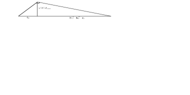
Figure 7: A geometric interpretation of the conditioning length

Thus, the conditioning length is defined so that $\sqrt{n}\,d_{rms}$ is the geometric mean between $l_{\mathcal{P}}$ and the sum of the projections of the set $\{\,{\bf{r}}_{j}\,\}_{1}^{n}$ onto the corresponding vectors of the set $\{\,{\bf{k}}_{j}\,\}_{1}^{n}$, as illustrated in Fig. 7.

5.5 A Rotation of the Isotropic Set as a Rigid Body

Since a rigid-body rotation of a set of isotropic points preserves isotropy, we can find the orientation of this set, as parameterized by the angle of rotation $\alpha$, that renders $z$ a minimum, for a given manipulator posture. Let this rotation be ${\bf{R}}(\alpha)$, which can be expressed as [11]

$${\bf{R}}(\alpha)=(\cos\alpha){\bf{1}}+(\sin\alpha){\bf{E}}$$ (45)

with E defined in eq.(12). Thus, upon rotating the set $\mathcal{K}$ through an angle $\alpha$ about its centroid $C$ or, equivalently, about the operation point $P$, the isotropic matrix K becomes $\tilde{{\bf{K}}}$, and is given by

$$\tilde{{\bf{K}}}=\left[\begin{array}[]{cccc}1&1&\cdots&1\\ {\bf{E}}{\bf{R}}(\alpha){\bf{k}}_{1}&{\bf{E}}{\bf{R}}(\alpha){\bf{k}}_{2}&\cdots&{\bf{E}}{\bf{R}}(\alpha){\bf{k}}_{n}\end{array}\right]$$ (46a)

The objective function $$z$$ then becomes

$$z=\frac{1}{2n}\left[{\rm tr}(\overline{{\bf{J}}}~{}\overline{{\bf{J}}}^{T})-2{\rm tr}(\overline{{\bf{J}}}\tilde{{\bf{K}}}^{T})+{\rm tr}(\tilde{{\bf{K}}}\tilde{{\bf{K}}}^{T})\right]\quad\rightarrow\quad\min_{\alpha}$$ (46b)

Before setting up the normality conditions for the problem at hand, we note that

$$\tilde{{\bf{K}}}\tilde{{\bf{K}}}^{T}=\left[\begin{array}[]{cc}n&(\sum_{1}^{n}{\bf{k}}_{i})^{T}{\bf{E}}^{T}{\bf{R}}^{T}(\alpha)\\ {\bf{R}}(\alpha){\bf{E}}\sum_{1}^{n}{\bf{k}}_{i}&{\bf{R}}(\alpha){\bf{E}}(\sum_{1}^{n}{\bf{k}}_{i}{\bf{k}}_{i}^{T}){\bf{E}}^{T}{\bf{R}}^{T}(\alpha)\end{array}\right]$$ (47)

which can be shown to reduce to

$$\tilde{{\bf{K}}}\tilde{{\bf{K}}}^{T}=\left[\begin{array}[]{cc}n&(\sum_{1}^{n}{\bf{k}}_{i})^{T}{\bf{E}}^{T}{\bf{R}}^{T}(\alpha)\\ {\bf{R}}(\alpha){\bf{E}}\sum_{1}^{n}{\bf{k}}_{i}&k^{2}{\bf{1}}_{2\times 2}\end{array}\right]$$ (50)

and hence,

$$\frac{\partial[{\rm tr}(\tilde{{\bf{K}}}\tilde{{\bf{K}}}^{T})]}{\partial\alpha}=0$$

On the other hand, $\overline{{\bf{J}}}$ is independent of $\alpha$, and hence, the normality condition of problem (46b) reduces to

$$\frac{\partial z}{\partial\alpha}\equiv-\frac{1}{n}\left[{\rm tr}\left(\overline{{\bf{J}}}\frac{\partial\tilde{{\bf{K}}}^{T}}{\partial\alpha}\right)\right]=0$$ (51)

We calculate below the partial derivative required above:

$$\frac{\partial\tilde{{\bf{K}}}}{\partial\alpha}=\left[\begin{array}[]{cccc}0&0&\cdots&0\\ {\bf{R}}^{\prime}(\alpha){\bf{E}}{\bf{k}}_{1}&{\bf{R}}^{\prime}(\alpha){\bf{E}}{\bf{k}}_{2}&\cdots&{\bf{R}}^{\prime}(\alpha){\bf{E}}{\bf{k}}_{n}\end{array}\right]$$ (54)

where ${\bf{R}}^{\prime}(\alpha)$ can be expressed, in light of relation (45), as

$${\bf{R}}^{\prime}(\alpha)={\bf{E}}{\bf{R}}(\alpha)$$

and hence,

$$\frac{\partial\tilde{{\bf{K}}}}{\partial\alpha}=\left[\begin{array}[]{cccc}0&0&\cdots&0\\ {\bf{E}}{\bf{R}}(\alpha){\bf{E}}{\bf{k}}_{1}&{\bf{E}}{\bf{R}}(\alpha){\bf{E}}{\bf{k}}_{2}&\cdots&{\bf{E}}{\bf{R}}(\alpha){\bf{E}}{\bf{k}}_{n}\end{array}\right]$$ (57)

whence,

$${\rm tr}\left(\overline{{\bf{J}}}\frac{\partial\tilde{{\bf{K}}}^{T}}{\partial\alpha}\right) = \lambda{\rm tr}\{\sum_{1}^{n}{\bf{E}}{\bf{r}}_{j}[{\bf{E}}{\bf{R}}(\alpha){\bf{E}}{\bf{k}}_{j}]^{T}\}=\lambda\sum_{1}^{n}{\bf{r}}_{j}^{T}{\bf{E}}^{T}{\bf{E}}{\bf{R}}(\alpha){\bf{E}}{\bf{k}}_{j}$$

$$= \lambda\sum_{1}^{n}{\bf{r}}_{j}^{T}{\bf{R}}(\alpha){\bf{E}}{\bf{k}}_{j}$$

Now, under the plausible assumption that $l_{\mathcal{P}}$ is finite, $\lambda\neq 0$, and hence, the normality condition (51) reduces to

$$\sum_{1}^{n}{\bf{r}}_{j}^{T}{\bf{R}}(\alpha){\bf{E}}{\bf{k}}_{j}=0$$

Further, substitution of expression (45) into the above expression leads to

$$(\cos\alpha)\sum_{1}^{n}{\bf{r}}_{j}^{T}{\bf{E}}{\bf{k}}_{j}-(\sin\alpha)\sum_{1}^{n}{\bf{r}}_{j}^{T}{\bf{k}}_{j}=0$$ (58)

Therefore, the value of $\alpha$ minimizing the distance of $\overline{{\bf{J}}}$ to $\tilde{{\bf{K}}}(\alpha)$ is, for the given posture $\mathcal{P}$,

$$\alpha=\arctan\left[\frac{\sum_{1}^{n}{\bf{r}}_{j}^{T}{\bf{E}}{\bf{k}}_{j}}{\sum_{1}^{n}{\bf{r}}_{j}^{T}{\bf{k}}_{j}}\right]\equiv\arctan\left[\frac{(1/n)\sum_{1}^{n}{\bf{r}}_{j}^{T}{\bf{E}}{\bf{k}}_{j}}{(1/n)\sum_{1}^{n}{\bf{r}}_{j}^{T}{\bf{k}}_{j}}\right]$$ (59)

Thus, the angle $\alpha$ through which the given isotropic set $\mathcal{K}$ is to be rotated in order to obtain the conditioning length of the manipulator pose $\mathcal{P}$ is given as the $\arctan$ function of the ratio of a numerator $N$ to a denominator $D$, whose geometric interpretations are straightforward: $D$ is simply the mean value of the projections of the ${\bf{r}}_{j}$ vectors onto their corresponding ${\bf{k}}_{j}$ vectors. Now, since ${\bf{E}}{\bf{k}}_{j}$ is vector ${\bf{k}}_{j}$ rotated $90^{\circ}$ counterclockwise, $N$ is the mean value of the projections of the ${\bf{r}}_{j}$ vectors onto their corresponding ${\bf{E}}{\bf{k}}_{j}$ vectors. We can call the latter the transverse projections of the said vectors. Once we have found the optimum value $\alpha_{\rm opt}$ of $\alpha$ for a given manipulator posture, we redefine, for conciseness,

$${\bf{K}}\quad\leftarrow\quad\tilde{{\bf{K}}}(\alpha_{\rm opt})$$ (60)

With $\alpha_{\rm opt}$ known, $l_{\mathcal{P}}$ is readily computed from eq.(44). Now, if we regard the columns of $\overline{{\bf{J}}}$ and K as 3-dimensional vectors, then a rotation Q of the corresponding 3-dimensional space about an axis normal to the plane of the sets $\{\,{\bf{r}}_{j}\,\}_{1}^{n}$ and $\{\,{\bf{k}}_{j}\,\}_{1}^{n}$ through an angle $q$ can be represented as

$${\bf{Q}}=\left[\begin{array}[]{cccc}1&{\bf{0}}^{T}\\ {\bf{0}}&{\bf{R}}(q)\end{array}\right]$$ (63)

where ${\bf{R}}(q)$ is a $2\times 2$ rotation matrix similar to ${\bf{R}}(\alpha)$, as defined in eq.(45). Hence, under rotation Q, $\overline{{\bf{J}}}$ and K change as described below:

$${\bf{Q}}\overline{{\bf{J}}} = \left[\begin{array}[]{cc}1&{\bf{0}}^{T}\\ {\bf{0}}&{\bf{R}}(q)\end{array}\right]\left[\begin{array}[]{cccc}1&1&\cdots&1\\ (1/l_{\mathcal{P}})~{}{\bf{E}}{\bf{r}}_{1}&(1/l_{\mathcal{P}})~{}{\bf{E}}{\bf{r}}_{2}&\cdots&(1/l_{\mathcal{P}})~{}{\bf{E}}{\bf{r}}_{n}\end{array}\right]$$ (68)

$$= \left[\begin{array}[]{cccc}1&1&\cdots&1\\ {\bf{R}}(q){\bf{E}}{\bf{r}}_{1}&{\bf{R}}(q){\bf{E}}{\bf{r}}_{2}&\cdots&{\bf{R}}(q){\bf{E}}{\bf{r}}_{n}\end{array}\right]$$ (71)

$${\bf{Q}}{\bf{K}} = \left[\begin{array}[]{cccc}1&1&\cdots&1\\ {\bf{R}}(q){\bf{E}}{\bf{k}}_{1}&{\bf{R}}(q){\bf{E}}{\bf{k}}_{2}&\cdots&{\bf{R}}(q){\bf{E}}{\bf{k}}_{n}\end{array}\right]$$ (74)

Now it is apparent that $z$, as defined in eq.(41), is invariant under a rotation ${\bf{R}}(q)$ of the sets $\mathcal{S}$ and $\mathcal{K}$. Indeed, under such a rotation,

$$z_{{\bf{Q}}} \equiv \frac{1}{2}\frac{1}{n}{\rm tr}({\bf{Q}}\overline{{\bf{J}}}\overline{{\bf{J}}}^{T}{\bf{Q}}^{T}-{\bf{Q}}{\bf{K}}\overline{{\bf{J}}}^{T}{\bf{Q}}^{T}-{\bf{Q}}\overline{{\bf{J}}}{\bf{K}}^{T}{\bf{Q}}^{T}+{\bf{Q}}{\bf{K}}{\bf{K}}^{T}{\bf{Q}}^{T})$$

$$= \frac{1}{2}\frac{1}{n}{\rm tr}[{\bf{Q}}(\overline{{\bf{J}}}\overline{{\bf{J}}}^{T}-{\bf{K}}\overline{{\bf{J}}}^{T}-\overline{{\bf{J}}}{\bf{K}}^{T}+{\bf{K}}{\bf{K}}^{T}){\bf{Q}}^{T}]$$

If we recall relation (20a), the above expression becomes

$$z_{{\bf{Q}}} \equiv \frac{1}{2}\frac{1}{n}{\rm tr}[{\bf{Q}}^{T}{\bf{Q}}(\overline{{\bf{J}}}\overline{{\bf{J}}}^{T}-{\bf{K}}\overline{{\bf{J}}}^{T}-\overline{{\bf{J}}}{\bf{K}}^{T}+{\bf{K}}{\bf{K}}^{T})]=z$$ (75)

We thus have proven

Lemma 5

The distance of $\overline{{\bf{J}}}$ to K is invariant under a rotation of the sets $\mathcal{S}$ and $\mathcal{K}$.

5.6 The Optimum Posture

It is now apparent that we can always orient the $\mathcal{K}$ set optimally, so that, for any posture $\mathcal{P}$, $\overline{{\bf{J}}}$ lies a minimum distance from the corresponding matrix K. Moreover, by virtue of Lemma 5, a rotation of the whole manipulator as a rigid body about its first joint, i.e., a motion of the manipulator with all its joints but the first one locked, does not affect $z$. That is, $z$ is a function of only $\{\,\theta_{i}\,\}_{2}^{n}$, which can thus be termed the set of conditioning-joint variables, the associated joints being the conditioning joints. Now we aim at finding the optimum posture ${\mathcal{P}}_{o}$ that yields a dimensionless Jacobian $\overline{{\bf{J}}}$ lying a minimum distance to the reference matrix K. To this end, we adopt a given set $\mathcal{K}$ at a given orientation at the outset, which thus leads to a constant matrix K in the process of finding ${\mathcal{P}}_{o}$, the optimum orientation of $\mathcal{K}$ being readily determined from eq.(59) once ${\mathcal{P}}_{o}$ has been found. Thus, in the derivations that follow, $\theta_{1}$ can be set arbitrarily equal to zero, or to any other constant value, for that matter. We now aim at solving the problem

$$z=\frac{1}{2}\frac{1}{n}{\rm tr}(\overline{{\bf{J}}}\overline{{\bf{J}}}^{T}-2{\bf{K}}\overline{{\bf{J}}}^{T}+{\bf{K}}{\bf{K}}^{T})\quad\rightarrow\quad\min_{\{\theta_{i}\}_{2}^{n}}$$ (76)

An attempt to solving this problem using the approach of the foregoing sections proved to be impractical. Indeed, since $z$ depends on the set of conditioning joint variables both via the set $\{\,{\bf{r}}_{j}\,\}_{1}^{n}$ and via $\lambda$, this dependence leads to a normality condition that does not lend itself to a closed-form solution. As a consequence, the said normality condition does not lead to a direct geometric interpretation of the optimum posture.

We thus follow a different approach here. For each posture, the value of $\lambda$ is computed using eq.(44), while $\alpha$ is computed with the eq.(59). With the foregoing expressions substituted into the expression of $z$ given in eq.(76), the corresponding normality conditions for angles ${\theta_{i}}^{n}_{2}$ yield a system of algebraic equations in the foregoing conditioning variables that are amenable to solutions using modern methods, like polynomial continuation, Gröbner bases, or resultant methods [12], that yield all roots of the problem at hand. These roots then lead to the globally-optimum posture ${\mathcal{P}}_{o}$.

5.7 The Characteristic Length

The optimum postures of a given manipulator, i.e., those with a Jacobian matrix closest to a corresponding model matrix K are thus found upon solving the optimization problem (76). Moreover, the conditioning length associated with the posture yielding a global minimum of the foregoing distance is defined as the characteristic length of the manipulator at hand. Prior to discussing some examples, we would like to find out whether the characteristic length thus found bears a minimality geometric property, e.g., whether the characteristic length is the minimum conditioning length of the manipulator over its whole workspace. To this end, we rewrite the objective function $z$ in the form

$$z=\frac{1}{2n}(\lambda^{2}nd_{\rm rms}^{2}-2\lambda\sum_{1}^{n}{\bf{k}}_{j}^{T}{\bf{r}}_{j}+\sum_{1}^{n}\|{\bf{k}}_{j}\|^{2})$$ (77)

Upon substitution of the sum $\sum_{1}^{n}{\bf{k}}_{j}^{T}{\bf{r}}_{j}$ in terms of the optimum value of $\lambda$ found in eq.(44) into eq.(77), we obtain

$$z=\frac{1}{2n}\sum_{1}^{n}\|{\bf{k}}_{j}\|^{2}-\frac{1}{2}\lambda^{2}d_{\rm rms}^{2}\equiv\frac{1}{2n}\sum_{1}^{n}\|{\bf{k}}_{j}\|^{2}-\frac{1}{2}\left(\frac{d_{\rm rms}}{l_{\mathcal{P}}}\right)^{2}$$ (78)

It is apparent from the above expression that minimizing $z$ is not equivalent to minimizing $l_{\mathcal{P}}$, but rather to maximizing the ratio $d_{\rm rms}/l_{\mathcal{P}}$. Hence, minimizing $z$ is equivalent to minimizing the inverse ratio, i.e., $l_{\mathcal{P}}/d_{\rm rms}$. In other words, minimizing $z$ is equivalent to minimizing the ratio of the conditioning length to the rms value of the distances of the joint centers from the operation point.

5.8 Examples: A Three-DOF Planar Manipulator

5.8.1 An Isotropic Manipulator

In the first example, we have $a_{1}=a_{2}=l$ and $a_{3}=\sqrt{3}\,l/3$, with the $\{\,{\bf{r}}_{j}\,\}_{1}^{3}$ vectors given by

$${\bf{r}}_{1}=l\left[\begin{array}[]{r}\cos(\theta_{1})+\cos(\theta_{12})+\cos(\theta_{123})\\ \sin(\theta_{1})+\sin(\theta_{12})+\sin(\theta_{123})\end{array}\right]{\rm~{},~{}}$$ (81)

$${\bf{r}}_{2}=l\left[\begin{array}[]{c}\cos(\theta_{12})+\cos(\theta_{123})\\ \sin(\theta_{12})+\sin(\theta_{123})\end{array}\right]{\rm~{},~{}}{\bf{r}}_{3}=\frac{\sqrt{3}l}{3}\left[\begin{array}[]{c}\cos(\theta_{123})\\ \sin(\theta_{123})\end{array}\right]$$ (86)

with the definition $\theta_{ij\ldots p}\equiv\theta_{i}+\theta_{j}+\ldots+p$. Moreover, the model matrix K used for this case is that found for the case of an isotropic set of three points, as discussed in Subsection 5.2, and reproduced below for quick reference:

$${\bf{K}}=\left[\begin{array}[]{ccc}1&1&1\\ -\sqrt{2}/2&-\sqrt{2}/2&~{}\sqrt{2}\\ ~{}\sqrt{6}/2&-\sqrt{6}/2&0\end{array}\right]$$ (87)

One optimum posture found with the procedure discussed in Subsection 5.6 is displayed in Fig. 9, the objective function attaining a minimum of zero at this posture, which means that the manipulator can match exactly an isotropic model matrix K within its workspace, the manipulator thus being termed isotropic. The objective function attains the values displayed in Fig. 9 over its whole workspace.

At the optimum posture, we have the values of the joint variables given below:

$$\theta_{1}=0^{\circ},\quad\theta_{2}=120^{\circ},\quad\theta_{3}=150^{\circ}$$

the conditioning length $l_{\mathcal{P}}$ being equal to $(\sqrt{6}/6)\,l$, which is thus the characteristic length of this manipulator, as found using an alternative approach in [5]. Moreover, the normalized Jacobian $\overline{{\bf{J}}}$ becomes

$$\overline{{\bf{J}}}=\left[\begin{array}[]{ccc}1&1&1\\ -\sqrt{2}/2&-\sqrt{2}/2&\sqrt{2}\\ \sqrt{6}/2&-\sqrt{6}/2&0\end{array}\right]$$

5.8.2 An Equilateral Manipulator

In the second example, we assume that all the link lengths are equal to $l$, and hence,

$${\bf{r}}_{1} = l\left[\begin{array}[]{r}\cos(\theta_{1})+\cos(\theta_{12})+\cos(\theta_{123})\\ \sin(\theta_{1})+\sin(\theta_{12})+\sin(\theta_{123})\end{array}\right]{\rm~{},~{}}{\bf{r}}_{2}=l\left[\begin{array}[]{c}\cos(\theta_{12})+\cos(\theta_{123})\\ \sin(\theta_{12})+\sin(\theta_{123})\end{array}\right]$$ (92)

$${\bf{r}}_{3} = l\left[\begin{array}[]{c}\cos(\theta_{123})\\ \sin(\theta_{123})\end{array}\right]$$ (95)

We call this manipulator equilateral.

For this case, we use the same model matrix K that we used in the previous example, for the manipulator has the same number of joints, and only one K was found—up to a reflection—for this number of joints. The minimization of the objective function leads to the optimum values

$$\theta_{1}=0^{\circ},\quad\theta_{2}=81.8^{\circ},\quad\theta_{3}=155.2^{\circ}$$

which correspond to a minimum value of $z=0.178$, the associated characteristic length being $l_{\mathcal{P}}=0.563\,l$. The corresponding posture is displayed in Fig. 11, while the objective function, evaluated throughout the workspace of the manipulator, is displayed in Fig. 11.

Finally, the normalized Jacobian at the posture of Fig. 11 is

$$\overline{{\bf{J}}}=\left[\begin{array}[]{ccc}1&1&1\\ -0.268&-0.268&1.489\\ 1.061&-0.714&-0.966\end{array}\right]$$

5.9 The Isocontours of the Objective Function

The minimum of the objective function $z$ corresponds to the posture closest to isotropy. At the other end of the spectrum, the maximum of this function is attained at those singular postures whereby the rank of the Jacobian matrix is two. The curves of constant $z$-values, termed the isocontours of the manipulator, can be used to define a performance index to compare manipulators, as described below. The isocontours were obtained with Surfer, a Surface Mapping System, for $\theta_{2}$ and $\theta_{3}\in[0,\,2\pi]$. The isocontours of the isotropic manipulator, of the first example, are displayed in Fig. 13; those of the equilateral manipulator in Fig. 13.

It is apparent from the two foregoing figures that the isocontours can be closed or open. If closed, the curves enclose the optimum point in the space of conditioning joints; in the second case, the curves are periodic. The shape of the closed curves, additionally, provides useful information on the manipulator performance: For the isotropic manipulator, when the objective function is below $0.25$, the curves are close to circular, as shown in Fig. 15; for the equilateral manipulator, these curves are close to elliptical, as shown in Fig. 15. This means that, in the neighborhood of an optimum, the isocontours behave in a way similar to the manipulability ellipsoid [3]: An isotropic manipulator entails a manipulability ellipsoid with semiaxes of identical lengths.

6 Applications to Design and Control

Manipulators are designed for a family of tasks, more so than for a specific task—manipulator design for a specific task defeats the purpose of using a manipulator, in the first place! The first step in designing a manipulator, moreover, is to dimension its links. It is apparent that from a purely geometric viewpoint, the link lengths are not as important as the link-length ratios. Once these ratios are optimally determined, the link lengths can be obtained based on requirements such as maximum reach for a given family of tasks, e.g., whether the manipulator is being used for cleaning a wide-body or a regional aircraft. Now, the maximum reach is directly proportional to the $d_{\rm rms}$ value of the distance of the joint centers to the operation point at the optimum posture, and hence, we can obtain the optimum link-length ratios by assuming that $d_{\rm rms}$ is equal to one unit of length. This means that minimizing the objective function $z$, as given by eq.(78), is equivalent to minimizing the normalized conditioning length $l_{\mathcal{P}}$, where the normalization is carried out upon dividing this length by $d_{\rm rms}$. Furthermore, when deciding on the manipulator link-length ratios, we may specify a certain useful workspace region as a subset of the whole workspace. How to decide on the boundaries of this region is something that can be done based on the value of $z$, so that we can establish a maximum allowable value of $z$, say $z_{M}<z_{\rm max}$, that we are willing to tolerate so as to keep the manipulator far enough from singularities. In this regard, the area enclosed by the isocontour $z=z_{M}$ will give a nondimensional measure, and hence, a measure independent of the scale of the manipulator, of the useful workspace region.

Under no constraints on the link-length ratios, for example, the designer should choose the optimum ratios of the isotropic manipulator of Fig. 9. On the other hand, when the manipulator is given, and it is desired to control it so as to keep it away from singularities, function $z$ can be used again as a measure of the distance to singularities: when $z$ attains its global maximum, the manipulator finds itself at a rank-two singularity. A rank-one singularity occurs at a local maximum. Furthermore, if a manipulator of given link-length ratios—e.g., one out of a family of manipulators with identical architectures, but of different scales, like the Puma 260, 560, or 760—is to be used for arc welding, then (a) the most suitable dimensions should be chosen according with the dimensions of the welding seam, and (b) the seam should be placed with respect to the manipulator in such a way that, as the EE traces that seem with the welding nozzle at a given angle with the seam, the objective function $z$ must remain within a maximum value $z_{M}$. This means that the seam should lie as close as possible to the optimum posture of Fig. 11. Furthermore, note that a rotation of the manipulator about the first joint axis, while keeping its other two joints locked, does not perturb $z$, and hence, a set of optimum postures is available. This set comprises the circle centered at the center of the first joint, of radius $d_{1}$—the distance of the operation point $P$ to the center of the first joint. This circle is similar to the isotropy circle of isotropic manipulators [5], and thus, can be termed the conditioning circle. Therefore, a good criterion to properly place the seam is that the seam lie as close a spossible to the conditioning circle.

Finally, while detecting singularities of nonredundant robots is a rather trivial task, detecting those of their redundant counterparts is more involved, and a fast estimation of the proximity of a given manipulator posture to singularity is always advantageous. This estimation is provided by the objective function $z$ proposed in this paper.

7 Conclusions

The conditioning length $l_{\mathcal{P}}$ was defined for a given posture of a planar manipulator. This concept allows us to normalize the Jacobian matrix so as to render it in nondimensional form. We base the definition of the characteristic length on an objective function $z$ that gives a geometric significance to the conditioning length. Moreover, the objective function introduced here is defined as a measure of the distance of the normalized—nondimensional—Jacobian matrix to an isotropic reference matrix. Isotropic sets of points in the plane are defined as well as operations on these sets. The paper is limited to planar manipulators, the treatment of spatial manipulators being as yet to be reported.

8 Illustrations

Figure 3: (a) Rotation of an isotropic set $\mathcal{S}$ and (b) union of $\mathcal{S}$ with its rotated image

Figure 8: An isotropic posture with $\theta_{1}=0^{\circ}$

Figure 9: Objective function of the isotropic manipulator

Figure 10: The posture closest to isotropy with $\theta_{1}=0^{\circ}$

Figure 11: Objective function of the equilateral manipulator

Figure 12: The isocontours of the objective function of the isotropic manipulator

Figure 13: The isocontours of the objective function of the equilateral manipulator

Figure 14: The isocontours closset to isotropy of the objective function of the isotropic manipulator

Figure 15: The isocontours closest to isotropy of the objective function of the equilateral manipulator

References

- [1] Vinogradov, I. B., Kobrinski, A. E., Stepanenko, Y. E., and Tives, L. T., “Details of Kinematics of Manipulators with the Method of Volumes”, Mekhanika Mashin, No. 27–28, 1971, pp. 5-16. In Russian.
- [2] Kumar, A. V., and Waldron, K.J., “The Workspace of a Mechanical Manipulator”, ASME Journal of Mechanical Design, 1981, pp. 665–672.
- [3] Yoshikawa, T., “Manipulability of Robotic Mechanisms”, The Int. J. Robotics Res., Vol. 4, No. 2, 1985 pp. 3–9.
- [4] Lee, J., Duffy, J. and Hunt, K., “A Pratical Quality Index Based on the Octahedral Manipulator”, The International Journal of Robotic Research, Vol. 17, No. 10, October 1998, pp. 1081–1090.
- [5] Angeles, J., Fundamentals of Robotic Mechanical Systems, Springer-Verlag, New York, 1997.
- [6] Golub, G. H. and Van Loan, C. F., Matrix Computations, The John Hopkins University Press, Baltimore, 1989.
- [7] Salisbury, J.K., and Craig, J. J., “Articulated Hands: Force Control and Kinematic Issues”, The Int. J. Robotics Res., Vol. 1, No. 1, 1982, pp. 4–17.
- [8] Angeles, J., and López-Cajún, C. S., “Kinematic Isotropy and the Conditioning Index of Serial Manipulators”, The Int. J. Robotics Res., Vol. 11, No. 6, 1992, pp. 560–571.
- [9] Paden, B., and Sastry, S., “Optimal Kinematic Design of 6R Manipulator”, The Int. J. Robotics Res., Vol. 7, No. 2, 1988, pp. 43–61.
- [10] Ranjbaran, F., Angeles, J., Gonzáles-Palacios, M.A., and Patel, R.V., “The Mechanical Design of a Seven-Axes Manipulator with Kinematic Isotropy”, Journal of Intelligent and Robotic Systems, Vol. 14, 1995, pp. 21–41.
- [11] Bottema, O. and Roth, B. Theorical Kinematics, North-Holland Publishing, Co. Amsterdam, 1979.
- [12] J. Nielsen, and B. Roth, “Computational Methods in Mechanical Systems”, NATO ASI Series F, Vol. 161, Springer-Verlag, Heidelberg, 1998, 233–252.