Abstract

Results are presented for the leading two-loop contributions of ${\cal O}(\alpha_{t}\alpha_{s})$ to the masses and mixing effects in the Higgs sector of the MSSM with complex parameters. They are obtained in the Feynman-diagrammatic approach using on-shell renormalization. The full dependence on all complex phases is taken into account. The renormalization of the appropriate contributions of the Higgs-boson sector and the scalar top and bottom sector is discussed. Our numerical analysis for the lightest MSSM Higgs-boson mass is based on the new two-loop corrections, supplemented by the full one-loop result. The corrections induced by the phase variation in the scalar top sector are enhanced by the two-loop contributions. We find that the corresponding shift in $M_{h_{1}}$ can amount to $5\,\,\mathrm{GeV}$.

1 Introduction

The Higgs sector of the Minimal Supersymmetric Standard Model (MSSM) with two scalar doublets accommodates five physical Higgs bosons. In lowest order these are the light and heavy ${\cal CP}$-even $h$ and $H$, the ${\cal CP}$-odd $A$, and the charged Higgs bosons $H^{\pm}$. Higher-order contributions yield large corrections to the masses and couplings, and also induce ${\cal CP}$-violation leading to mixing between $h,H$ and $A$ in the case of general complex SUSY breaking parameters.

For the MSSM with real parameters (rMSSM) the status of higher-order corrections to the masses and mixing angles in the Higgs sector is quite advanced [1, 2, 3, 4, 5, 6, 7, 8, 9, 10]. In the case of the MSSM with complex parameters (cMSSM), the first more general investigations [11] were followed by evaluations in the effective potential approach [12] and with the renormalization-group-improved one-loop effective potential method [13, 14]. These results have been restricted to the corrections arising from the (s)fermion sector and some leading logarithmic corrections from the gaugino sector. Within the Feynman diagrammatic (FD) approach the one-loop leading $m_{t}^{4}$ corrections have been evaluated in Ref. [15]. Most recently a full one-loop calculation in the FD approach was presented [16] (further discussions on the effect of complex phases on Higgs boson masses can be found in Ref. [17]) and implemented in the program FeynHiggs [2, 7, 18, 16], which is publicly available. Another public code, CPsuperH [19], is based on the renormalization-group-improved effective potential approach [13, 14].

In this letter we improve our diagrammatic one-loop calculation [16] by providing the leading ${\cal O}(\alpha_{t}\alpha_{s})$ corrections of the Higgs-boson masses and mixings in the cMSSM obtained in the FD approach. Technically we calculate and renormalize the Higgs-boson self energies taking into account the general complex parameters of the appropriate part of the colored sector of the cMSSM. We provide numerical examples for the lightest cMSSM Higgs-boson mass and discuss the dependence on the phases in the scalar top sector and on the gluino mass parameter. The results presented in this paper will be included in the code FeynHiggs [20].

2 The Higgs-boson sector of the cMSSM

With the two Higgs doublets of the cMSSM decomposed in the following way,

$${\cal H}_{1}=\begin{pmatrix}H_{11}\\ H_{12}\end{pmatrix} =\begin{pmatrix}v_{1}+\tfrac{1}{\sqrt{2}}(\phi_{1}-i\chi_{1})\\ -\phi^{-}_{1}\end{pmatrix},$$

$${\cal H}_{2}=\begin{pmatrix}H_{21}\\ H_{22}\end{pmatrix} =e^{i\xi}\begin{pmatrix}\phi^{+}_{2}\\ v_{2}+\tfrac{1}{\sqrt{2}}(\phi_{2}+i\chi_{2})\end{pmatrix},$$ (1)

the Higgs potential $V_{H}$ can be arranged as an expansion in powers of the field components,

$$V_{H} =-T_{\phi_{1}}\phi_{1}-T_{\phi_{2}}\phi_{2}-T_{\chi_{1}}\chi_{1}-T_{\chi_{2}}\chi_{2}$$

$$+\tfrac{1}{2}\begin{pmatrix}\phi_{1},\phi_{2},\chi_{1},\chi_{2}\end{pmatrix}{\mathbf{M}}_{\phi\phi\chi\chi}\begin{pmatrix}\phi_{1}\\ \phi_{2}\\ \chi_{1}\\ \chi_{2}\end{pmatrix}+\begin{pmatrix}\phi^{-}_{1},\phi^{-}_{2}\end{pmatrix}{\mathbf{M}}_{\phi^{\pm}\phi^{\pm}}\begin{pmatrix}\phi^{+}_{1}\\ \phi^{+}_{2}\end{pmatrix}+\cdots,$$ (2)

where the ellipses stand for higher powers in the Higgs-boson fields. In Eq. (2) the tadpoles appear as the coefficients of the linear terms, and the bilinear terms contain the neutral and charged mass matrices ${\mathbf{M}}_{\phi\phi\chi\chi}$ and ${\mathbf{M}}_{\phi^{\pm}\phi^{\pm}}$. Tadpoles and mass matrices are conveniently rewritten in terms of the physical components $h,H,A,H^{\pm}$ and the Goldstone components $G,G^{\pm}$. Details about the tadpole coefficients and the mass matrices can be found in Ref. [16].

Eq. (2) introduces a possible new phase $\xi$ between the two Higgs doublets. The potential $V_{H}$ contains the real soft breaking terms $\tilde{m}_{1}^{2}$ and $\tilde{m}_{2}^{2}$ (with $m_{1}^{2}\equiv\tilde{m}_{1}^{2}+|\mu|^{2}$, $m_{2}^{2}\equiv\tilde{m}_{2}^{2}+|\mu|^{2}$) and the generally complex soft breaking parameter $m_{12}^{2}$, entering the mass matrices and tadpoles in Eq. (2). With the help of a Peccei-Quinn transformation [21], $\mu$ and $m_{12}^{2}$ can be redefined [22] such that the complex phase of $m_{12}^{2}$ vanishes. In the following we will therefore treat $m_{12}^{2}$ as a real parameter, i.e. $|m_{12}^{2}|=m_{12}^{2}$. Together with the requirement that the minimum of $V_{H}$ is located at $v_{1}$ and $v_{2}$, all tadpoles are zero at lowest order.

Investigating the Higgs potential beyond the tree level, renormalization has to be applied to the mass matrices and the tadpoles, introducing counterterms according to the loop expansion up to second order,

$${\mathbf{M}}_{hHAG} \to{\mathbf{M}}_{hHAG}+\delta{\mathbf{M}}_{hHAG}^{(1)}+\delta{\mathbf{M}}_{hHAG}^{(2)}$$ (3)

$${\mathbf{M}}_{H^{\pm}G^{\pm}} \to{\mathbf{M}}_{H^{\pm}G^{\pm}}+\delta{\mathbf{M}}_{H^{\pm}G^{\pm}}^{(1)}+\delta{\mathbf{M}}_{H^{\pm}G^{\pm}}^{(2)}$$ (4)

$$T_{i} \to T_{i}+\delta T_{i}^{(1)}+\delta T_{i}^{(2)}~{},\quad i=h,H,A~{},$$ (5)

where the mass matrices and tadpoles are obtained from those in Eq. (2) by a rotation to the physical states. The leading ${\cal O}(\alpha_{t}\alpha_{s})$ contributions to the Higgs-boson self-energies are obtained in the limit of vanishing gauge couplings and neglecting the dependence on the external momentum. The bottom Yukawa coupling, appearing in the charged Higgs-boson self-energy, is also neglected. Since for the leading two-loop terms the Goldstone-boson parts of Eqs. (3) and (4) do not contribute (see also the discussion in Ref. [16]), mass renormalization at the two-loop level reduces to the counterterms

$$\delta M_{H^{\pm}}^{2(2)}\qquad{\rm and}\qquad\delta{\mathbf{M}}_{hHA}^{(2)}=\begin{pmatrix}\delta m_{h}^{2(2)}&\delta m_{hH}^{2(2)}&\delta m_{hA}^{2(2)}\\[5.0pt] \delta m_{hH}^{2(2)}&\delta m_{H}^{2(2)}&\delta m_{HA}^{2(2)}\\[5.0pt] \delta m_{hA}^{2(2)}&\delta m_{HA}^{2(2)}&\delta m_{A}^{2(2)}\end{pmatrix}~{}.$$ (6)

The renormalized Higgs-boson self-energies, denoted as $\hat{\Sigma}_{ij}(p^{2})$ with $i,j=h,H,A,H^{\pm}$, are expanded into a one-loop and a two-loop part,

$$\hat{\Sigma}_{ij}(p^{2})=\hat{\Sigma}^{(1)}_{ij}(p^{2})+\hat{\Sigma}^{(2)}_{ij}(0)~{}.$$ (7)

The complete one-loop part has been obtained in Ref. [16], and the two-loop part is evaluated at vanishing external momentum, as explained above. The renormalized two-loop self-energies

$$\hat{\Sigma}_{ij}^{(2)}(0) =\Sigma_{ij}^{(2)}(0)-\delta m_{ij}^{2(2)},\quad i,j=h,H,A$$ (8)

$$\hat{\Sigma}_{H^{+}H^{-}}^{(2)}(0) =\Sigma_{H^{+}H^{-}}^{(2)}(0)-\delta M_{H^{\pm}}^{2(2)}$$ (9)

involve the unrenormalized Higgs-boson self-energies $\Sigma_{ij}^{(2)}(0)$, containing the one-loop subrenormalization, and the counterterms of Eq. (6).

The entries $\delta m_{ij}^{2(2)}$ ($i,j=h,H,A$) of the counterterm matrix in Eq. (6) are not all independent, but can be expressed in terms of $\delta M_{H^{\pm}}^{2(2)}$ and $\delta T_{i}^{(2)}$. As explained e.g. in Ref. [2], $M_{H^{\pm}}^{2}$ and $T_{i}$ are the only independent parameters in the Higgs potential that have to be renormalized for the evaluation of the ${\cal O}(\alpha_{t}\alpha_{s})$ terms. Correspondingly, it is sufficient to impose renormalization conditions for the tadpoles and for the charged Higgs-boson mass:

• The tadpoles are fixed by the requirement that the minimum of the Higgs potential is not shifted, yielding at the two-loop level

  $$T_{i}^{(2)}+\delta T_{i}^{(2)}=0 \Rightarrow \delta T_{i}^{(2)}=-T_{i}^{(2)}~{},~{}i=h,H,A~{}.$$ (10)

• The mass square of the charged Higgs boson, $M_{H^{\pm}}^{2}$, is fixed by an on-shell condition yielding the following counterterm at the two-loop level:

  $$\mathop{\mathrm{Re}}\hat{\Sigma}_{H^{+}H^{-}}(0)=0 \Rightarrow \delta M_{H^{\pm}}^{2(2)}=\Sigma_{H^{+}H^{-}}^{(2)}(0)~{}.$$ (11)

With these, the counterterms for the neutral mass matrix are now determined in the following way,

$$\delta m_{h}^{2(2)} =c_{\alpha-\beta}^{2}\,\delta M_{H^{\pm}}^{2(2)}+\frac{e\,s_{\alpha-\beta}}{4M_{Z}c_{\mathrm{w}}s_{\mathrm{w}}}\Bigl{[}\bigl{(}s_{\alpha-2\beta}-3s_{\alpha}\bigr{)}\delta T_{\phi_{1}}^{(2)}+\bigl{(}c_{\alpha-2\beta}+3c_{\alpha}\bigr{)}\delta T_{\phi_{2}}^{(2)}\Bigr{]}~{},$$ (12)

$$\delta m_{hH}^{2(2)} =\frac{s_{2\alpha-2\beta}}{2}\delta M_{H^{\pm}}^{2(2)}+\frac{e\,c_{\alpha-\beta}}{4M_{Z}c_{\mathrm{w}}s_{\mathrm{w}}}\Bigl{[}\bigl{(}s_{2\alpha-\beta}+c_{2\alpha-2\beta}s_{\beta}\bigr{)}\delta T_{\phi_{1}}^{(2)}-\frac{c_{2\alpha-3\beta}+3c_{2\alpha-\beta}}{2}\delta T_{\phi_{2}}^{(2)}\Bigr{]}~{},$$ (13)

$$\delta m_{H}^{2(2)} =s^{2}_{\alpha-\beta}\,\delta M_{H^{\pm}}^{2(2)}+\frac{e\,c_{\alpha-\beta}}{4M_{Z}c_{\mathrm{w}}s_{\mathrm{w}}}\Bigl{[}\bigl{(}c_{\alpha-2\beta}-3c_{\alpha}\bigr{)}\delta T_{\phi_{1}}^{(2)}-\bigl{(}s_{\alpha-2\beta}+3s_{\alpha}\bigr{)}\delta T_{\phi_{2}}^{(2)}\Bigr{]}~{},$$ (14)

$$\delta m_{AH}^{2(2)} =-\frac{e\,c_{\alpha-\beta}}{2M_{Z}c_{\mathrm{w}}s_{\mathrm{w}}}\delta T_{A}^{(2)}~{},$$ (15)

$$\delta m_{Ah}^{2(2)} =\frac{e\,s_{\alpha-\beta}}{2M_{Z}c_{\mathrm{w}}s_{\mathrm{w}}}\delta T_{A}^{(2)}~{},$$ (16)

$$\delta m_{A}^{2(2)} =\delta M_{H^{\pm}}^{2(2)}~{}.$$ (17)

We have used $s_{x}\equiv\sin(x)$, $c_{x}\equiv\cos(x)$ as abbreviations. The angle $\alpha$ diagonalizes the $\phi_{1}\phi_{2}$ mass matrix at tree-level, $T_{\phi_{1}}$ and $T_{\phi_{2}}$ denote the $H$ and $h$ tadpoles, respectively, in the limit of $\alpha\to 0$, which are the tadpoles in Eq. (2).

The calculation of the unrenormalized self-energies and tadpoles at ${\cal O}(\alpha_{t}\alpha_{s})$ requires the evaluation of genuine two-loop diagrams and one-loop graphs with counterterm insertions. Example diagrams for the neutral Higgs-boson self-energies are depicted in Fig. 1, and for the charged Higgs boson in Fig. 2. Examples for the tadpole diagrams are displayed in Fig. 3. The complete set of contributing Feynman diagrams has been generated with the program FeynArts [23]; tensor reduction and the evaluation of traces was done with support of the programs OneCalc and TwoCalc [24], yielding analytic expressions in terms of the scalar one-loop functions $A_{0},B_{0}$ [25] and two-loop vacuum integrals [26]. The numerical evaluation was performed with the help of the program LoopTools [27].

Figure 1: Examples of generic two-loop diagrams and diagrams with counterterm insertion for the Higgs-boson self-energies ($\phi=h,H,A$; $\;i,j,k,l=1,2$).

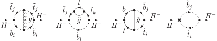
Figure 2: Examples of generic two-loop diagrams and diagrams with counterterm insertion for the charged Higgs-boson self-energy ($i,j,k=1,2$).

Figure 3: Examples of generic two-loop diagrams and diagrams with counterterm insertion for the Higgs-boson tadpoles, ($\phi=h,H,A$; $\;i,j,k=1,2$).

The renormalized self-energies determine the dressed propagators of the Higgs fields, from which masses and mixing properties at higher order are derived. The self-energies have an impact on the location of the poles and thus on the Higgs particle masses, which are in general different from their tree-level values. Only the charged Higgs boson mass $M_{H^{\pm}}$ is not shifted, owing to the on-shell renormalization condition (11).

The non-diagonal self-energies are responsible for mixing in the neutral Higgs system. In the presence of complex parameters all three neutral ${\cal CP}$ eigenstates $h,H,A$ can mix. The $3\times 3$ propagator matrix, $\Delta_{hHA}(p^{2})$, is obtained by inverting the renormalized irreducible two-point function,

$$\Delta_{hHA}(p^{2})=-\left(\hat{\Gamma}_{hHA}(p^{2})\right)^{-1},$$ (18)

where

$$\hat{\Gamma}_{hHA}(p^{2}) =i\left[p^{2}{\rm 1\mskip-4.25mul}-{\mathbf{M}}_{\mathrm{n}}(p^{2})\right],$$ (19)

$${\mathbf{M}}_{\mathrm{n}}(p^{2}) =\begin{pmatrix}m_{h}^{2}-\hat{\Sigma}_{hh}(p^{2})&-\hat{\Sigma}_{hH}(p^{2})&-\hat{\Sigma}_{hA}(p^{2})\\ -\hat{\Sigma}_{hH}(p^{2})&m_{H}^{2}-\hat{\Sigma}_{HH}(p^{2})&-\hat{\Sigma}_{HA}(p^{2})\\ -\hat{\Sigma}_{hA}(p^{2})&-\hat{\Sigma}_{HA}(p^{2})&m_{A}^{2}-\hat{\Sigma}_{AA}(p^{2})\end{pmatrix}.$$ (20)

The masses of the three Higgs-boson mass eigenstates, $h_{1}$, $h_{2}$, $h_{3}$, ordered according to $M_{h_{1}}\leq M_{h_{2}}\leq M_{h_{3}}$, are given by the real parts of the poles of $\Delta_{hHA}(p^{2})$ or, equivalently, of the roots of the determinant of the two-point vertex function, ${\rm det}[\hat{\Gamma}_{hHA}(p^{2})]=0$. The quantities $m_{h},m_{H},m_{A}$ in Eq. (20) are the masses of $h,H,A$ at the tree-level, respectively.

3 The colored sector of the cMSSM

For the evaluation of the ${\cal O}(\alpha_{t}\alpha_{s})$ two-loop contributions to the tadpoles and self-energies, a renormalization of the one-loop contributions from the scalar top ($\tilde{t}$) and bottom ($\tilde{b}$) sector is needed, giving rise to the counterterms for one-loop subrenormalization (see Figs. 1–3). The bilinear part of the $\tilde{t}$ and $\tilde{b}$ Lagrangian,

$${\cal L}_{\tilde{t}/\tilde{b}\text{ mass}} =-\begin{pmatrix}{{\tilde{t}}_{L}}^{\dagger},{{\tilde{t}}_{R}}^{\dagger}\end{pmatrix}{\mathbf{M}}_{\tilde{t}}\begin{pmatrix}{\tilde{t}}_{L}\\ {\tilde{t}}_{R}\end{pmatrix}-\begin{pmatrix}{{\tilde{b}}_{L}}^{\dagger},{{\tilde{b}}_{R}}^{\dagger}\end{pmatrix}{\mathbf{M}}_{\tilde{b}}\begin{pmatrix}{\tilde{b}}_{L}\\ {\tilde{b}}_{R}\end{pmatrix}~{},$$ (21)

contains the stop and sbottom mass matrices ${\mathbf{M}}_{\tilde{t}}$ and ${\mathbf{M}}_{\tilde{b}}$, given by

$${\mathbf{M}}_{\tilde{q}} =\begin{pmatrix}M_{L}^{2}+m_{q}^{2}+M_{Z}^{2}c_{2\beta}(T_{q}^{3}-Q_{q}s_{\mathrm{w}}^{2})&m_{q}X_{q}^{*}\\[1.99997pt] m_{q}X_{q}&M_{\tilde{q}_{R}}^{2}+m_{q}^{2}+M_{Z}^{2}c_{2\beta}Q_{q}s_{\mathrm{w}}^{2}\end{pmatrix}~{},\quad q=t,\,b~{},$$ (22)

$${\rm with}$$

$$X_{q} =A_{q}-\mu^{*}\kappa~{},\qquad\kappa=\{\cot\beta,\tan\beta\}\quad{\rm for}\quad q=t,b~{}.$$ (23)

$Q_{{q}}$ and $T_{q}^{3}$ denote charge and isospin of $q$, and $A_{q}$ is the trilinear soft-breaking parameter. The mass matrix can be diagonalized with the help of a unitary transformation ${{\mathbf{U}}}_{\tilde{q}}$, which can be parametrized by a mixing angle ${\theta}_{\tilde{q}}$ and a phase $\varphi_{\tilde{q}}$,

$${\mathbf{D}}_{\tilde{q}} ={\mathbf{U}}_{\tilde{q}}\,{\mathbf{M}}_{\tilde{q}}\,{{\mathbf{U}}}_{\tilde{q}}^{\dagger}=\begin{pmatrix}m_{\tilde{q}_{1}}^{2}&0\\ 0&m_{\tilde{q}_{2}}^{2}\end{pmatrix}\,,\quad\ {{\mathbf{U}}}_{\tilde{q}}=\begin{pmatrix}U_{\tilde{q}_{11}}&U_{\tilde{q}_{12}}\\ U_{\tilde{q}_{21}}&U_{\tilde{q}_{22}}\end{pmatrix}=\begin{pmatrix}\cos{\theta}_{\tilde{q}}&e^{i{\varphi}_{\tilde{q}}}\sin{\theta}_{\tilde{q}}\\ -e^{-i{\varphi}_{\tilde{q}}}\sin{\theta}_{\tilde{q}}&\cos{\theta}_{\tilde{q}}\end{pmatrix}~{}.$$ (24)

The mass eigenvalues depend only on $|X_{q}|$.

Taking into account complex phases, the renormalization in the $\tilde{t}$ sector is somewhat more involved than in the case of real parameters [2, 3, 28]. In the cMSSM the $\tilde{t}$ sector is described in terms of five real parameters (where we assume that $\mu$ and $\tan\beta$ are defined via other sectors): the real soft SUSY-breaking parameters $M_{L}^{2}$ and $M_{{\tilde{t}}_{R}}^{2}$, the absolute value and complex phase of the trilinear coupling, $A_{t}=|A_{t}|e^{i\varphi_{A_{t}}}$, and the top Yukawa coupling $\lambda_{t}$ that can be chosen to be real. Instead of the quantities $M_{L}^{2}$, $M_{{\tilde{t}}_{R}}^{2}$ and $\lambda_{t}$, in the on-shell scheme applied in this paper we choose the on-shell squark masses $m_{\tilde{t}_{1}}^{2}$, $m_{\tilde{t}_{2}}^{2}$ and the top-quark mass $m_{t}$ as independent parameters.

The following renormalization conditions are imposed:

• The top-quark mass is defined on-shell, yielding the one-loop counterterm $\delta m_{t}$:

  $$\delta m_{t}=\frac{1}{2}m_{t}\bigl{(}\widetilde{\text{Re}}{\Sigma}_{t}^{L}(m_{t}^{2})+\widetilde{\text{Re}}{\Sigma}_{t}^{R}(m_{t}^{2})+2\widetilde{\text{Re}}{\Sigma}_{t}^{S}(m_{t}^{2})\bigr{)}~{},$$ (25)

  referring to the Lorentz decomposition of the self energy ${\Sigma}_{t}$

  $${\Sigma}_{t}(k) =\not\!k{\omega}_{-}{\Sigma}_{t}^{L}(k^{2})+\not\!k{\omega}_{+}{\Sigma}_{t}^{R}(k^{2})+m_{t}{\Sigma}_{t}^{S}(k^{2})+m_{t}\gamma_{5}{\Sigma}_{t}^{PS}(k^{2})$$ (26)

  into a left-handed, a right-handed, a scalar and a pseudoscalar part, ${\Sigma}_{t}^{L}$, ${\Sigma}_{t}^{R}$, ${\Sigma}_{t}^{S}$ and ${\Sigma}_{t}^{PS}$, respectively. $\widetilde{\text{Re}}$ denotes the real part with respect to contributions from the loop integral, but leaves the complex couplings unaffected.

• The stop masses are also determined via on-shell conditions [2, 28], yielding

  $$\delta m_{\tilde{t}_{i}}^{2} =\widetilde{\text{Re}}\Sigma_{\tilde{t}_{ii}}(m_{{\tilde{t}}_{i}}^{2})\quad\ \text{with}\quad\ i=1,\,2~{}.$$ (27)

• The third condition affects the stop mixing angle and phase, or equivalently, the $A_{t}$ parameter. Rewriting the squark mass matrix in terms of the mass eigenvalues and the mixing angle and phase using Eq. (24),

  $${{\mathbf{M}}}_{\tilde{t}} =\begin{pmatrix}\cos^{2}\theta_{\tilde{t}}m_{\tilde{t}_{1}}^{2}+\sin^{2}\theta_{\tilde{t}}m_{\tilde{t}_{2}}^{2}&e^{i{\varphi}_{\tilde{t}}}\sin\theta_{\tilde{t}}\cos\theta_{\tilde{t}}(m_{\tilde{t}_{1}}^{2}-m_{\tilde{t}_{2}}^{2})\\ e^{-i{\varphi}_{\tilde{t}}}\sin\theta_{\tilde{t}}\cos\theta_{\tilde{t}}(m_{\tilde{t}_{1}}^{2}-m_{\tilde{t}_{2}}^{2})&\sin^{2}\theta_{\tilde{t}}m_{\tilde{t}_{1}}^{2}+\cos^{2}\theta_{\tilde{t}}m_{\tilde{t}_{2}}^{2}\end{pmatrix}\,,$$ (28)

  yields the counterterm matrix $\delta{{\mathbf{M}}}_{\tilde{t}}$ by introducing counterterms $\delta m_{\tilde{t}_{1}}^{2},\delta m_{\tilde{t}_{2}}^{2}$ for the masses and $\delta\theta_{\tilde{t}},\delta\varphi_{\tilde{t}}$ for the angles. For the case of the real MSSM one obtains the counterterm for the mixing angle,

  $$\mbox{rMSSM:}\qquad(m^{2}_{\tilde{t}_{1}}-m^{2}_{\tilde{t}_{2}})\,\delta\theta_{\tilde{t}}=[{\mathbf{U}}_{\tilde{t}}\,\delta{\mathbf{M}}_{\tilde{t}}\,{\mathbf{U}}_{\tilde{t}}^{\dagger}]_{12}\equiv\delta Y_{\tilde{t}}\,,$$ (29)

  for which the following renormalization condition has been used [3, 28]:

  $$\mbox{rMSSM:}\qquad\delta Y_{\tilde{t}}=\frac{1}{2}\,[{\text{Re}}{\Sigma}_{\tilde{t}_{12}}(m_{\tilde{t}_{1}}^{2})+{\text{Re}}{\Sigma}_{\tilde{t}_{12}}(m_{\tilde{t}_{2}}^{2})]\,.$$ (30)

  Generalizing Eq. (29) to the complex case, we obtain

  $$\delta Y_{\tilde{t}}=[{\mathbf{U}}_{\tilde{t}}\,\delta{\mathbf{M}}_{\tilde{t}}\,{\mathbf{U}}_{\tilde{t}}^{\dagger}]_{12}=(m^{2}_{\tilde{t}_{1}}-m^{2}_{\tilde{t}_{2}})\,e^{i\varphi_{\tilde{t}}}\,(\delta\theta_{\tilde{t}}+i\sin\theta_{\tilde{t}}\cos\theta_{\tilde{t}}\,\,\delta\varphi_{\tilde{t}})~{},$$ (31)

  and impose, as a generalization of Eq. (30), the condition

  $$\delta Y_{\tilde{t}}=\frac{1}{2}\,[\widetilde{\text{Re}}{\Sigma}_{\tilde{t}_{12}}(m_{\tilde{t}_{1}}^{2})+\widetilde{\text{Re}}{\Sigma}_{\tilde{t}_{12}}(m_{\tilde{t}_{2}}^{2})]\,,$$ (32)

  which now corresponds to two separate conditions for the real and imaginary part, or for $\delta\theta_{\tilde{t}}$ and $\delta\varphi_{\tilde{t}}$, respectively.

  We adopt a scheme where $|A_{t}|$ and $\varphi_{A_{t}}$ are chosen as independent parameters. The two sets of parameters $\theta_{\tilde{t}}$, $\varphi_{\tilde{t}}$ and $|A_{t}|$, $\varphi_{A_{t}}$ are mutually related via Eq. (22) and Eq. (28). The off-diagonal entries of the corresponding counterterm matrices yield

  $$(A_{t}^{*}-\mu\cot\beta)\,\delta m_{t}+m_{t}\,\delta A_{t}^{*}=U^{*}_{\tilde{t}_{11}}U_{\tilde{t}_{12}}(\delta m_{\tilde{t}_{1}}^{2}-\delta m_{\tilde{t}_{2}}^{2})+U^{*}_{\tilde{t}_{11}}U_{\tilde{t}_{22}}\delta Y_{t}+U_{\tilde{t}_{12}}U^{*}_{\tilde{t}_{21}}\delta Y_{t}^{*}~{}.$$ (33)

  As a result, we obtain for $\delta|A_{t}|$ and $\delta\varphi_{A_{t}}$

  $$\delta|A_{t}| =\frac{1}{m_{t}}\text{Re}[e^{i\varphi_{A_{t}}}K_{t}]~{},$$ (34)

  $$\delta\varphi_{A_{t}} =-\frac{1}{m_{t}|A_{t}|}\text{Im}[e^{i\varphi_{A_{t}}}K_{t}]~{},$$ (35)

  with

  $$K_{t} =-(A_{t}^{*}-\mu\cot\beta)\delta m_{t}+U_{\tilde{t}_{11}}^{*}U_{\tilde{t}_{12}}(\delta m_{\tilde{t}_{1}}^{2}-\delta m_{\tilde{t}_{2}}^{2})+U_{\tilde{t}_{11}}^{*}U_{\tilde{t}_{22}}\delta Y_{t}+U_{\tilde{t}_{12}}U_{\tilde{t}_{21}}^{*}\delta Y_{t}^{*}~{}.$$

In the scalar bottom sector, we also encounter five real parameters (with $\mu$ and $\tan\beta$ defined via other sectors): the real soft-breaking parameters $M_{L}^{2}$ and $M_{{\tilde{b}}_{R}}^{2}$, the absolute value and phase of the trilinear coupling $A_{b}$, and the bottom Yukawa coupling $\lambda_{b}$ that can be chosen to be real (for the set of corrections presented in this paper $\lambda_{b}$ does not enter, as explained above). SU$(2)$ invariance requires the “left-handed” soft-breaking parameters in the stop and the sbottom sector to be identical (denoted as $M_{L}^{2}$). In the evaluation of the ${\cal O}(\alpha_{t}\alpha_{s})$ contributions to the Higgs-boson self-energies, the counterterms of the sbottom sector appear only in the self-energy of the charged Higgs boson. In our approximation, where the $b$-quark mass is neglected, $\tilde{b}_{L}$ and $\tilde{b}_{R}$ do not mix, and $\tilde{b}_{R}$ decouples and does not contribute. The charged Higgs-boson self-energy thus depends only on a single parameter of the sbottom sector, which can be chosen as the squark mass $m_{\tilde{b}_{L}}$. The parameter $m_{\tilde{b}_{L}}$ should be regarded simply as the upper left entry in the $\tilde{b}$ mass matrix, not as a physical $\tilde{b}$ pole mass (see also Ref. [3, 28]). By means of SU$(2)$ invariance, the corresponding mass counterterm is already determined:

$$\delta m_{\tilde{b}_{L}}^{2}=|U_{\tilde{t}_{11}}|^{2}\delta m_{\tilde{t}_{1}}^{2}+|U_{\tilde{t}_{12}}|^{2}\delta m_{\tilde{t}_{2}}^{2}-U_{\tilde{t}_{12}}^{*}U_{\tilde{t}_{22}}\delta Y_{t}-U_{\tilde{t}_{12}}U_{\tilde{t}_{22}}^{*}\delta Y_{t}^{*}-2m_{t}\delta m_{t}~{}.$$ (36)

With the set of renormalization constants determined in Eqs. (25), (27), (34), (35) and (36) the counterterms for the diagonal and non-diagonal (s)quark self-energies as well as for all Higgs-boson–(s)quark vertices are at our disposal for the one-loop subrenormalization. An explicit list of the counterterms will be provided in a detailed forthcoming publication [20].

Finally, at ${\cal O}(\alpha_{t}\alpha_{s})$ gluinos appear as virtual particles at the two-loop level (hence, no renormalization is needed). The corresponding soft-breaking gluino mass parameter $M_{3}$ is in general complex,

$$M_{3}=|M_{3}|e^{i\varphi_{\tilde{g}}}\quad(\text{with the gluino mass}~{}m_{\tilde{g}}=|M_{3}|)~{}.$$ (37)

The phase can be absorbed by a redefinition of the gluino Majorana spinor such that it appears only in the gluino couplings, but not in the mass term.

4 Numerical results

We illustrate the effects of the two-loop contributions in terms of the mass of the lightest neutral Higgs boson, $M_{h_{1}}$, evaluated on the basis of Eq. (20) with the entries from Eq. (7). The results for physical observables are affected only by certain combinations of the complex phases. In particular, the ${\cal O}(\alpha_{t}\alpha_{s})$ corrections presented in this paper depend only on the combinations [22, 29]

$$\mu\,A_{t}\,\left(m_{12}^{2}\right)^{*}\mbox{~{}~{}~{}and~{}~{}~{}}A_{t}\,M_{3}^{*}~{}.$$ (38)

As discussed above, we have transformed our parameters such that the complex phase of $m_{12}^{2}$ vanishes. Therefore our two-loop results depend on the phases of the parameters $A_{t}$, $\mu$ and $M_{3}$, which we denote as $\varphi_{A_{t}}$, $\varphi_{\mu}$ and $\varphi_{\tilde{g}}$, respectively. We do not consider the variation of complex phases that enter only via one-loop contributions.

In the context of a detailed phenomenological analysis of the cMSSM parameter space the existing constraints on ${\cal CP}$-violating parameters from experimental bounds for the electric dipole moments (EDMs) [30, 31] are of interest. While SM contributions enter only at the three-loop level, due to its complex phases the cMSSM can contribute to the EDMs already at one-loop order. The complex phases appearing in the cMSSM are experimentally constrained by their contribution to the EDMs of heavy quarks [32], of the electron and the neutron (see [33, 34] and references therein), and of deuterium [35]. One finds that in particular the phase $\varphi_{\mu}$ is tightly constrained (in the convention where the phase of the gaugino mass parameter $M_{2}$ is set to zero). The bounds on the phases of the third-generation trilinear couplings, on the other hand, are much weaker.

Since the complex phases appear in our two-loop result only in the combinations given in Eq. (38), we can conveniently choose $\varphi_{\mu}=0$, so that in our numerical analysis only $\varphi_{A_{t}}$ and $\varphi_{\tilde{g}}$ are varied. In order to illustrate the possible effects of complex phases we will show below results for $\varphi_{\tilde{g}}$, $\varphi_{A_{t}}$ varied over the full parameter range.

Our numerical analysis has been performed for the following set of parameters (if not indicated differently):

$$M_{\rm SUSY}=1000\,\,\mathrm{GeV},\;|A_{t}|=|A_{b}|=|A_{\tau}|=1000\,\,\mathrm{GeV},\;\varphi_{A_{b}}=\varphi_{A_{\tau}}=0,\;$$

$$\mu=1000\,\,\mathrm{GeV},\;M_{2}=500\,\,\mathrm{GeV},\;M_{1}=(5s_{\mathrm{w}}^{2})/(3c_{\mathrm{w}}^{2})\,M_{2},\;m_{\tilde{g}}=1000\,\,\mathrm{GeV},$$

$$M_{H^{\pm}}=500\,\,\mathrm{GeV},\;\tan\beta=10,\;m_{t}=174.3\,\,\mathrm{GeV}~{}.$$ (39)

$M_{\rm SUSY}$ denotes the diagonal soft SUSY-breaking parameters in the sfermion mass matrices that are chosen to be equal to each other. We do not consider higher values of $\tan\beta$, which in general enhance the SUSY contributions to the EDMs.

We first discuss the dependence of $M_{h_{1}}$ on the phase in the scalar top sector. Since the leading one-loop result in the limit $M_{H^{\pm}}\gg M_{Z}$ depends only on the absolute value $|X_{t}|\equiv|A_{t}-\mu^{*}/\tan\beta|$ (implying that only the combination $\varphi_{A_{t}}+\varphi_{\mu}$ enters, in accordance with Eq. (38)), it is useful to analyze the dependence of the result on $\varphi_{A_{t}}$ as well as on $\varphi_{X_{t}}$. In Fig. 4 we show the lightest Higgs-boson mass as a function of $\varphi_{A_{t}}$ (left) and of $\varphi_{X_{t}}$ (right) for $|X_{t}|=1.5\,\,\mathrm{TeV}$ (upper row) and $|X_{t}|=2.5\,\,\mathrm{TeV}$ (lower row). $|A_{t}|$ is chosen such that for vanishing phases it is equal in the left and right plot of each row. A variation of $\varphi_{A_{t}}$ for fixed $\mu$ and $\tan\beta$ changes the absolute value of $X_{t}$ and thus the masses of the scalar top quarks. Changing $\varphi_{X_{t}}$, on the other hand, leaves the masses of the scalar tops invariant (see Sect. 3), but changes $A_{t}$. Therefore, in the right plots the $\tilde{t}$ masses are constant ($m_{\tilde{t}_{1}}=770\,\,\mathrm{GeV}$ and $m_{\tilde{t}_{2}}=1210\,\,\mathrm{GeV}$). We compare in Fig. 4 the one-loop result for $M_{h_{1}}$ (dotted line) with the new result that includes the ${\cal O}(\alpha_{t}\alpha_{s})$ contributions (solid line).

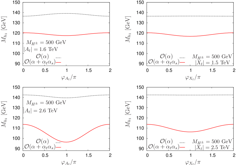
Figure 4: In the left column $M_{h_{1}}$ is given as a function of $\varphi_{A_{t}}$ for $|A_{t}|=1.6\,\,\mathrm{TeV}$ (upper plot) and $|A_{t}|=2.6\,\,\mathrm{TeV}$ (lower plot). In the right column $M_{h_{1}}$ is given as a function of $\varphi_{X_{t}}$ for $|X_{t}|=1.5\,\,\mathrm{TeV}$ (upper plot) and $|X_{t}|=2.5\,\,\mathrm{TeV}$ (lower plot). The other parameters are as given in Eq. (39) and $\varphi_{\tilde{g}}=0$. The one-loop results (dashed line) are compared with the results including the ${\cal O}(\alpha_{t}\alpha_{s})$ corrections (solid line).

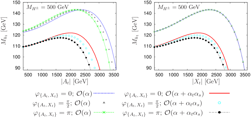
Figure 5: $M_{h_{1}}$ as a function of $|A_{t}|$ (left plot) and $|X_{t}|$ (right plot) for $\varphi_{X_{t}},\varphi_{A_{t}}=0,\pi/2,\pi$. The other parameters are as given in Eq. (39) and $\varphi_{\tilde{g}}=0$. The one-loop results are compared with the results including the ${\cal O}(\alpha_{t}\alpha_{s})$ corrections.

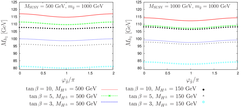
Figure 6: $M_{h_{1}}$ at ${\cal O}(\alpha_{t}\alpha_{s})$ as a function of $\varphi_{\tilde{g}}$ for $M_{\rm SUSY}=500\,\,\mathrm{GeV}$ (left) and $M_{\rm SUSY}=1000\,\,\mathrm{GeV}$ (right) with $M_{H^{\pm}}=150,500\,\,\mathrm{GeV}$, $\tan\beta=3,5,10$ and $\varphi_{A_{t}}=0$.

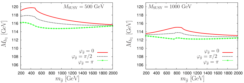
Figure 7: $M_{h_{1}}$ at ${\cal O}(\alpha_{t}\alpha_{s})$ as a function of $m_{\tilde{g}}$ for $M_{\rm SUSY}=500\,\,\mathrm{GeV}$ (left) and $M_{\rm SUSY}=1000\,\,\mathrm{GeV}$ (right) with $\varphi_{\tilde{g}}=0,\pi/2,\pi$ and $\varphi_{A_{t}}=0$.

Fig. 4 shows that the two-loop contributions lead to a reduction of $M_{h_{1}}$ of $\sim 20\,\,\mathrm{GeV}$, in accordance with the results in the rMSSM [1, 2]. The dependence on the complex phases $\varphi_{A_{t}}$ and $\varphi_{X_{t}}$ is much more pronounced in the two-loop result than in the one-loop case. This fact can easily be understood from the discussion above: for the relatively large $M_{H^{\pm}}$ chosen in Fig. 4 the one-loop result is dominated by contributions involving only the absolute value $|X_{t}|$. Therefore the dependence of the one-loop result on $\varphi_{X_{t}}$ is very weak (right column of Fig. 4), while the dependence on $\varphi_{A_{t}}$ arises to good approximation only from its effect on $|X_{t}|$. At the two-loop level, on the other hand, the contributions with internal gluinos depend on the phase of $(A_{t}\,M_{3}^{*})$, see Eq. (38). This induces an asymmetry of the leading corrections to $M_{h_{1}}$ with respect to $X_{t}$ (see Refs. [2, 4] for a discussion in the rMSSM).

The impact of the phases $\varphi_{A_{t}}$, $\varphi_{X_{t}}$ is obviously enhanced for larger values of $|A_{t}|$ and $|X_{t}|$. In Fig. 5 we show the dependence of $M_{h_{1}}$ on $|A_{t}|$ (left) and $|X_{t}|$ (right) for $\varphi_{A_{t}},\varphi_{X_{t}}=0,\pi/2,\pi$, respectively. Concerning the dependence on $|X_{t}|$, at the one-loop level the results are indistinguishable for the three values of $\varphi_{X_{t}}$, in agreement with the one-loop results in Fig. 4. Varying $\varphi_{A_{t}}$, on the other hand, results in a shift of the position of the maximum of $M_{h_{1}}$ in the one-loop result (left plot). At the two-loop level, the position and size of the maximum value of $M_{h_{1}}$ is significantly affected both by $\varphi_{A_{t}}$ and $\varphi_{X_{t}}$, in accordance with the discussion above.

We now investigate the dependence of $M_{h_{1}}$ on the phase of the gluino mass parameter, keeping the phase of $A_{t}$ fixed at $\varphi_{A_{t}}=0$. This means that only the second term in Eq. (38) is affected by the phase variation, while so far we had studied the combined effect of both terms in Eq. (38). Fig. 6 displays the variation of $M_{h_{1}}$ with $\varphi_{\tilde{g}}$ for $M_{\rm SUSY}=500\,\,\mathrm{GeV}$ (left) and $M_{\rm SUSY}=1000\,\,\mathrm{GeV}$ (right). $M_{H^{\pm}}$ is set to $150,500\,\,\mathrm{GeV}$, and $\tan\beta=3,5,10$. The dependence on the gluino phase (for $\varphi_{A_{t}}=0$) is relatively weak for the set of parameters chosen in Fig. 6, yielding shifts in $M_{h_{1}}$ below $\sim 2\,\,\mathrm{GeV}$. For larger $M_{H^{\pm}}$ the dependence is slightly stronger than for small $M_{H^{\pm}}$ values. In all cases a minimum of $M_{h_{1}}$ is reached for $\varphi_{\tilde{g}}=\pi$. Larger effects of the phase of the gluino mass parameter than the ones shown in the example of Fig. 6 would occur for larger values of $|A_{t}|$, as a consequence of Eq. (38).

In Fig. 7 the result for $M_{h_{1}}$ is shown as a function of $m_{\tilde{g}}$ for $\varphi_{\tilde{g}}=0,\pi/2,\pi$ (and $\varphi_{A_{t}}=0$). $M_{\rm SUSY}$ is set to $500\,\,\mathrm{GeV}$ (left) and $1000\,\,\mathrm{GeV}$ (right). The phase dependence is strongest around the thresholds $m_{\tilde{g}}=m_{\tilde{t}_{1}}-m_{t}$ and $m_{\tilde{g}}=m_{\tilde{t}_{2}}-m_{t}$. For the chosen set of parameters the thresholds correspond to $m_{\tilde{g}}=177\,\,\mathrm{GeV}$ (not shown) and $m_{\tilde{g}}=487\,\,\mathrm{GeV}$ for $M_{\rm SUSY}=500\,\,\mathrm{GeV}$, and to $m_{\tilde{g}}=760\,\,\mathrm{GeV}$ and $m_{\tilde{g}}=915\,\,\mathrm{GeV}$ for $M_{\rm SUSY}=1000\,\,\mathrm{GeV}$. The change in $M_{h_{1}}$ induced by the phase variation can amount up to $4\,\,\mathrm{GeV}$ in the threshold area for the parameters chosen in Fig. 7.

5 Conclusions

We have presented results for the leading ${\cal O}(\alpha_{t}\alpha_{s})$ contributions to the dressed Higgs-boson propagators in the MSSM with complex parameters, obtained in the Feynman-diagrammatic approach using an on-shell type renormalization scheme. In the Higgs sector a two-loop renormalization has to be carried out for the mass of the charged Higgs boson and the three tadpoles. The renormalization of the scalar top and bottom sector at the one-loop level involves a renormalization of the complex phase $\varphi_{A_{t}}$.

Concerning the explicit numerical results we have focused on the lightest Higgs-boson mass, $M_{h_{1}}$. This is of interest in view of the current exclusion bounds [36, 37] and possible high-precision measurements of the properties of a light Higgs boson at the next generation of colliders [38, 39, 40]. The ${\cal O}(\alpha_{t}\alpha_{s})$ corrections yield a large downward shift in $M_{h_{1}}$, in accordance with the well-known result from the rMSSM. We find that the impact of the complex phases $\varphi_{A_{t}}$ and $\varphi_{X_{t}}$ is significantly enhanced by the two-loop contributions, which is a consequence in particular of diagrams involving internal gluinos. We find that varying the complex phases of the scalar top sector and of the gluino mass parameter can induce shifts in $M_{h_{1}}$ of up to $\sim 5\,\,\mathrm{GeV}$ even in cases where the one-loop result shows hardly any dependence on the phases. The result for $M_{h_{1}}$ for $\varphi_{A_{t}},\varphi_{\tilde{g}}\neq 0,\pi$ is found to lie in the intervals given by $\pm|A_{t}|,\pm|M_{3}|$. The effects of the complex phases of the ${\cal O}(\alpha_{t}\alpha_{s})$ corrections can also be enhanced in the threshold region where the gluino mass is approximately equal to the sum of the top-quark mass and the mass of one of the scalar top quarks.

The new results of ${\cal O}(\alpha_{t}\alpha_{s})$ will be implemented into the Fortran code FeynHiggs  [2, 7, 18, 16]. A detailed description, including a comparison of different renormalization schemes for the scalar top sector and a more elaborate discussion of Higgs-boson masses and mixings will be presented in a forthcoming publication [20], as well as a comparison with the results based on the renormalization-group improved effective-potential approach [14, 19].

Acknowledgements

We thank T. Hahn and D. Stöckinger for helpful discussions. The work of S.H. was partially supported by CICYT (grant FPA2006–02315). Work supported in part by the European Community’s Marie-Curie Research Training Network under contract MRTN-CT-2006-035505 ‘Tools and Precision Calculations for Physics Discoveries at Colliders’

References

• [1] S. Heinemeyer, W. Hollik and G. Weiglein, Phys. Rev. D 58 (1998) 091701, hep-ph/9803277; Phys. Lett. B 440 (1998) 296, hep-ph/9807423.
• [2] S. Heinemeyer, W. Hollik and G. Weiglein, Eur. Phys. J. C 9 (1999) 343. hep-ph/9812472.
• [3] S. Heinemeyer, W. Hollik, H. Rzehak and G. Weiglein, Eur. Phys. J. C 39 (2005) 465, hep-ph/0411114.
• [4] S. Heinemeyer, W. Hollik and G. Weiglein, Phys. Lett. B 455 (1999) 179, hep-ph/9903404. M. Carena, H. Haber, S. Heinemeyer, W. Hollik, C. Wagner, and G. Weiglein, Nucl. Phys. B 580 (2000) 29, hep-ph/0001002.
• [5] R. Zhang, Phys. Lett. B 447 (1999) 89, hep-ph/9808299;
J. Espinosa and R. Zhang, JHEP 0003 (2000) 026, hep-ph/9912236;
G. Degrassi, P. Slavich and F. Zwirner, Nucl. Phys. B 611 (2001) 403, hep-ph/0105096;
R. Hempfling and A. Hoang, Phys. Lett. B 331 (1994) 99, hep-ph/9401219;
A. Brignole, G. Degrassi, P. Slavich and F. Zwirner, Nucl. Phys. B 631 (2002) 195, hep-ph/0112177; Nucl. Phys. B 643 (2002) 79, hep-ph/0206101;
J. Espinosa and R. Zhang, Nucl. Phys. B 586 (2000) 3, hep-ph/0003246;
J. Espinosa and I. Navarro, Nucl. Phys. B 615 (2001) 82, hep-ph/0104047;
G. Degrassi, A. Dedes and P. Slavich, Nucl. Phys. B 672 (2003) 144, hep-ph/0305127.
• [6] J. Casas, J. Espinosa, M. Quirós and A. Riotto, Nucl. Phys. B 436 (1995) 3, [Erratum-ibid. B 439 (1995) 466], hep-ph/9407389;
M. Carena, J. Espinosa, M. Quirós and C. Wagner, Phys. Lett. B 355 (1995) 209, hep-ph/9504316;
M. Carena, M. Quirós and C. Wagner, Nucl. Phys. B 461 (1996) 407, hep-ph/9508343.
• [7] G. Degrassi, S. Heinemeyer, W. Hollik, P. Slavich and G. Weiglein, Eur. Phys. J. C 28 (2003) 133, hep-ph/0212020.
• [8] S. Heinemeyer, W. Hollik and G. Weiglein, Phys. Rept. 425 (2006) 265. hep-ph/0412214.
• [9] B. Allanach, A. Djouadi, J. Kneur, W. Porod and P. Slavich, JHEP 0409 (2004) 044, hep-ph/0406166.
• [10] S. Martin, Phys. Rev. D 65 (2002) 116003, hep-ph/0111209; Phys. Rev. D 66 (2002) 096001, hep-ph/0206136; Phys. Rev. D 67 (2003) 095012, hep-ph/0211366; Phys. Rev. D 68 075002 (2003), hep-ph/0307101; Phys. Rev. D 70 (2004) 016005, hep-ph/0312092; Phys. Rev. D 71 (2005) 016012, hep-ph/0405022; Phys. Rev. D 71 (2005) 116004, hep-ph/0502168; hep-ph/0701051;
S. Martin and D. Robertson, Comput. Phys. Commun. 174 (2006) 133, hep-ph/0501132.
• [11] A. Pilaftsis, Phys. Rev. D 58 (1998) 096010, hep-ph/9803297; Phys. Lett. B 435 (1998) 88, hep-ph/9805373.
• [12] D. Demir, Phys. Rev. D 60 (1999) 055006, hep-ph/9901389;
S. Choi, M. Drees and J. Lee, Phys. Lett. B 481 (2000) 57, hep-ph/0002287;
T. Ibrahim and P. Nath, Phys. Rev. D 63 (2001) 035009, hep-ph/0008237; Phys. Rev. D 66 (2002) 015005, hep-ph/0204092.
• [13] A. Pilaftsis and C. Wagner, Nucl. Phys. B 553 (1999) 3, hep-ph/9902371.
• [14] M. Carena, J. Ellis, A. Pilaftsis and C. Wagner, Nucl. Phys. B 586 (2000) 92, hep-ph/0003180.
• [15] S. Heinemeyer, Eur. Phys. J. C 22 (2001) 521, hep-ph/0108059.
• [16] M. Frank, T. Hahn, S. Heinemeyer, W. Hollik, R. Rzehak and G. Weiglein, JHEP 02 (2007) 047, hep-ph/0611326.
• [17] H. Rzehak, PhD thesis: “Two-loop contributions in the supersymmetric Higgs sector”, Technische Universität München, 2005; see: nbn-resolving.de/
with urn: nbn:de:bvb:91-diss20050923-0853568146 .
• [18] S. Heinemeyer, W. Hollik and G. Weiglein, Comput. Phys. Commun. 124 (2000) 76, hep-ph/9812320; hep-ph/0002213; see www.feynhiggs.de .
• [19] J. Lee, A. Pilaftsis et al., Comput. Phys. Commun. 156 (2004) 283, hep-ph/0307377.
• [20] T. Hahn, S. Heinemeyer, W. Hollik, H. Rzehak and G. Weiglein, in preparation.
• [21] R. Peccei and H. Quinn, Phys. Rev. Lett. 38 (1977) 1440; Phys. Rev. D 16 (1977) 1791.
• [22] S. Dimopoulos and S. Thomas, Nucl. Phys. B 465 (1996) 23, hep-ph/9510220.
• [23] J. Küblbeck, M. Böhm and A. Denner, Comp. Phys. Comm. 60 (1990) 165;
T. Hahn, Comput. Phys. Comm. 140 (2001) 418, hep-ph/0012260;
The program is available via www.feynarts.de;
T. Hahn and C. Schappacher, Comput. Phys. Comm. 143 (2002) 54, hep-ph/0105349.
• [24] G. Weiglein, R. Scharf and M. Böhm, Nucl. Phys. B 416 (1994) 606, hep-ph/9310358;
G. Weiglein, R. Mertig, R. Scharf and M. Böhm, in New Computing Techniques in Physics Research 2, ed. D. Perret-Gallix (World Scientific, Singapore, 1992), p. 617.
• [25] G. ’t Hooft and M. Veltman, Nucl. Phys. B 153 (1979) 365.
• [26] A. Davydychev und J. Tausk, Nucl. Phys. B 397 (1993) 123;
F. Berends und J. Tausk, Nucl. Phys. B 421 (1994) 456.
• [27] T. Hahn, M. Perez-Victoria, Comput. Phys. Commun. 118 (1999) 153, hep-ph/9807565.
• [28] W. Hollik and H. Rzehak, Eur. Phys. J. C 32 (2003) 127, hep-ph/0305328.
• [29] M. Dugan, B. Grinstein and L. Hall, Nucl. Phys. B 255 (1985) 413.
• [30] W. Yao et al.  [Particle Data Group Collaboration], J. Phys. G 33 (2006) 1.
• [31] V. Barger, T. Falk, T. Han, J. Jiang, T. Li and T. Plehn, Phys. Rev. D 64 (2001) 056007, hep-ph/0101106.
• [32] W. Hollik, J. Illana, S. Rigolin and D. Stöckinger, Phys. Lett. B 416 (1998) 345, hep-ph/9707437; Phys. Lett. B 425 (1998) 322, hep-ph/9711322.
• [33] D. Demir, O. Lebedev, K. Olive, M. Pospelov and A. Ritz, Nucl. Phys. B 680 (2004) 339, hep-ph/0311314.
• [34] D. Chang, W. Keung and A. Pilaftsis, Phys. Rev. Lett. 82 (1999) 900 [Erratum-ibid.  83 (1999) 3972], hep-ph/9811202;
A. Pilaftsis, Phys. Lett. B 471 (1999) 174, hep-ph/9909485.
• [35] O. Lebedev, K. Olive, M. Pospelov and A. Ritz, Phys. Rev. D 70 (2004) 016003, hep-ph/0402023.
• [36] [LEP Higgs working group], Phys. Lett. B 565 (2003) 61, hep-ex/0306033; Eur. Phys. J. C 47 (2006) 547, hep-ex/0602042.
• [37] V. Abazov et al. [D0 Collaboration], Phys. Rev. Lett. 97 (2006) 121802, hep-ex/0605009; D0 Note 5331-CONF;
A. Abulencia et al. [CDF Collaboration], Phys. Rev. Lett. 96 (2006) 011802, hep-ex/0508051; CDF note 8676;
[CDF Collaboration], Phys. Rev. Lett. 96 (2006) 042003, hep-ex/0510065.
• [38] ATLAS Collaboration, Detector and Physics Performance Technical Design Report, CERN/LHCC/99-15 (1999), see:
atlasinfo.cern.ch/Atlas/GROUPS/PHYSICS/TDR/access.html ;
CMS Collaboration, Physics Technical Design Report, Volume 2. CERN/LHCC 2006-021, see: cmsdoc.cern.ch/cms/cpt/tdr/ .
• [39] V. Büscher and K. Jakobs, Int. J. Mod. Phys. A 20 (2005) 2523, hep-ph/0504099;
M. Schumacher, Czech. J. Phys. 54 (2004) A103; hep-ph/0410112.
• [40] J. Aguilar-Saavedra et al., TESLA TDR Part 3: “Physics at an $e^{+}e^{-}$ Linear Collider”, hep-ph/0106315, see: tesla.desy.de/tdr/;
T. Abe et al. [American Linear Collider Working Group Collaboration], hep-ex/0106056;
K. Abe et al. [ACFA Linear Collider Working Group Collaboration], hep-ph/0109166;
K. Ackermann et al., DESY-PROC-2004-01;
S. Heinemeyer et al., hep-ph/0511332.