The ontology of temperature in nonequilibrium systems

Abstract

The laws of thermodynamics provide a clear concept of the temperature for an equilibrium system in the continuum limit. Meanwhile, the equipartition theorem allows one to make a connection between the ensemble average of the kinetic energy and the uniform temperature. When a system or its environment is far from equilibrium, however, such an association does not necessarily apply. In small systems, the regression hypothesis may not even apply. Herein, we show that in small nonequilibrium systems, the regression hypothesis still holds though with a generalized definition of the temperature. The latter must now be defined for each such manifestation.

I Introduction

A lay person defines temperature as a measure of the heat contained in a body. This is not in conflict with a more rigorous thermodynamic definition based on the equipartition theorem when the body is in the continuum limit with respect to size and measurement time. But what is the temperature when these assumptions no longer hold? Is it useful to even try to describe small and/or nonequilibrium subsystems using an instantaneous temperature?

Experimentally, at least, temperature can be defined even for very fast and small systems using heat balances. For example, the temperature of a medium can be changed experimentally using a system excitation induced by a laser pulse or using a microwave field to heat the bath. The temperature in the local environment can be raised quickly by several to tens of degrees Centigrade in a few microseconds or less.Leeson et al. (2000) This elevated temperature can be sustained for milliseconds and subsequently decays back to the global environmental temperature within a time-scale of tens of milliseconds. Chen et al. (2005) Such $T$-jump experiments provide the time resolution needed for studying the kinetics of many processes —as in, e.g., protein- and peptide-folding, Snow et al. (2004); Chen et al. (2005); Leeson et al. (2000) and helix-coil transitions in peptides.Abbruzzetti et al. (2000); Munoz et al. (1997); Thompson et al. (1997); Davis and Harrington (1987) However, $T$-jumps can significantly influence the structural and dynamical properties of the systems under investigation. For example, solutions of colloidal and microgel particles change their size dramatically due to changes in temperature —and also pH.Jones and Lyon (2000); Wang et al. (2001); Jones and Lyon (2003); Fernandez-Nieves et al. (2000a); Garcia-Salinas et al. (2001); Fernandez-Nieves et al. (2001, 2000b, 2003) Indeed, such particles have been swelled by as much as an order of magnitude in just a few milliseconds.Pelton (2000); Wang et al. (2001); Fernandez-Nieves et al. (2002) Such environmental changes evidently affect the local and global structure and may enable coupling to additional heat sinks. At the very least, they require additional care in performing the heat balance to determine the temperature during the $T$-jump.

In order to assign a rigorous definition of the instantaneous temperature of a small (open or closed) system under nonequilibrium conditions, it is useful to partition it into a subsystem —specifying the properties of the material— and a bath —consisting of everything else. The latter may in turn also be open or closed depending on whether or not it is effectively interacting with an additional environment. When this bath is stationary, such as can be found in simple liquids or colloidal suspensions at equilibrium, the motion of the subsystem —as represented by an $n$-dimensional position coordinate $q$— can be accurately described by the generalized Langevin equation (GLE),Zwanzig (2001)

$$\ddot{q}(t)=-\frac{\partial V(q)}{\partial q}-\int_{0}^{t}{\gamma_{\rm th}(t-t^{\prime})\dot{q}(t^{\prime})dt^{\prime}}+\xi_{\rm th}(t)\;.$$ (1)

Here $V(q)$ is the potential of mean force (PMF), $\gamma_{\rm th}(t-t^{\prime})$ is the friction kernel representing the response of the solvent, $\xi_{\rm th}(t)$ is the random force due to the medium, and they obey the fluctuation-dissipation relation (FDR),

$$\left<\xi_{\rm th}(t)\xi_{\rm th}(t^{\prime})\right>=k_{\rm B}T\gamma_{\rm th}(t-t^{\prime})\;.$$ (2)

When the bath is nonstationary by way of exhibiting temporal (and spatial) changes in the ambient bath, Eq. (1) has been modified to the so-called irreversible GLE (iGLE):Hernandez and Somer (1999); Hernandez (1999)

$$\ddot{q}(t)=-\frac{\partial V(q)}{\partial q}-\int_{0}^{t}{\gamma(t,t^{\prime})\dot{q}(t^{\prime})dt^{\prime}}+\xi(t)\;,$$ (3)

$$\gamma(t,t^{\prime})=g(t)\gamma_{\rm th}(t-t^{\prime})g(t^{\prime})\;.$$ (4)

The function $g(t)$ modulating the friction kernel is completely determined by an irreversible process due to processes not otherwise included in the subsystem or bath. The stochastic force $\xi(t)\equiv g(t)\xi_{\rm th}(t)$ in the iGLE is modulated by the same function $g(t)$. The resulting nonstationary FDR is

$$\left<\xi(t)\xi(t^{\prime})\right>=k_{\rm B}T\gamma(t,t^{\prime})\;.$$ (5)

The system-bath dynamics characterized by the GLE and the iGLE have often been generalized to allow for the possibility of time-dependent or driven variations in the system temperature. In one set of approaches, the nonequilibrium behavior of the bath is introduced by way of an external stochastic force. This additional noise can drive the reaction coordinate $q$ directlyBanik et al. (2000) or by modulation of the local bath modes.Bravo et al. (1989); Chaudhuri et al. (2001, 2006) Although such a modulation may be caused by many different physically relevant mechanisms, the recurring requirement is that the external noise has no connection to the memory kernel $\gamma(t,t^{\prime})$ in the FDR. The latter can arise, for example, when the stochastic noise acting on the reacting subsystem and the local bath is independent. This requirement necessarily leads to a shift in the temperature. Refs. Bravo et al., 1989; Banik et al., 2000; Chaudhuri et al., 2001, 2006 have explored this issue within the Kramers theory, and the steady state of the nonequilibrium open subsystem was observed to lead to a new effective temperature.

However, if the system is truly in equilibrium with the overall bath, then the heat transfer leading to this temperature differential is presumably dissipated by bath modes not initially included in the local bath. A repartitioning of the environment into two sets —a nonequilibrium open reservoir and a global thermally equilibrated bath— have been suggested.Millonas and Ray (1995); Chaudhuri et al. (1998) External perturbations in the initial state of the former are relaxed to equilibrium through the coupling to the latter. (The FDR between the random forces and the memory kernel appears naturally in this case.) This coupling is stipulated by a specific Hamiltonian model of the bath, though primarily their work has specified the bath using the usual choice of a set of harmonic modes coupled by bilinear interactions. Each such mode is then assumed to approach its equilibrium value exponentially with a specified dissipation rate. Alternatively, the heat from the nonequilibrium local bath may be balanced directly in the iGLE through the ad hoc introduction of an effective heat sink which has indeed been seen to provide self-consistent constant-temperature dynamics.Shepherd and Hernandez (2002); Moix et al. (2004); Moix and Hernandez (2005)

Regardless, the requirement that the overall bath dissipate the system so quickly that constant temperature is always maintained is too severe. For example, it does not describe systems in which energy transport fluctuations to nearby local bath modes may be important. Nor does it account for (driven) temperature-ramped chemical reactions as has earlier been treated using a simple generalization of the iGLE.Somer and Hernandez (1999) That approach is restricted to the case of slow temperature variations as will be recapitulated in Sec. III. Thus the question remains as to whether a subsystem within a nonequilibrium environment can be characterized using an observable temperature, and if so, how to calculate or measure it.

In the current work, we investigate a generalized chemical process in which the nonequilibrium behavior of the chosen subsystem is influenced by a change in temperature of the environment that is in turn influenced by the response of the subsystem. In such a case, the environment itself can also persist in a nonequilibrium state. The model, therefore, consists of a hierarchy of three domains: a small-dimensional system, a nonequilibrium open “local” bath (see Fig. 1)

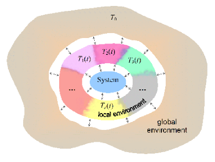
Figure 1: A hierarchical representation of a (sub)system under investigation which is immersed within a local nonequilibrium environment that is, in turn, interacting with a global equilibrium one. (Color online.)

strongly coupled to the system, and a “global” bath that is coupled to the local bath and at most weakly coupled to the system. Without loss of generality, the linear response of the local baths can be represented using an auxiliary model of harmonic oscillators coupled bilinearly to the system. The interaction between the local and global environments induces a time dependence in the parameters characterizing the local bath—viz., the effective masses of the oscillators, their frequencies and the coupling between the local bath and the system. Assuming that the effective temperature of each bath mode is observable, we investigate the connections between these variables and the system. The time dependence of the bath parameters can be specified according to the behavior of any particular physical problem, and so this theory can be applied quite generally as discussed above.

One important case for these problems (indeed it lies at the core of the discussion that follows) is the possibility that the local bath actually consists of several independent baths (or reservoirs). This separation can be viewed as a mathematical trick that enables one to demonstrate the possibility of invariances regardless of the specific representation. But it is also physically relevant. For example, two- and three- temperature models have been used to describe ultra-short laser pulse desorption experiments.Hohlfeld et al. (2000); Nest and Saalfrank (2004) Therein, the distinct reservoirs represent the adsorbate layer, the substrate phonons and the substrate electrons, respectively, and the times scales of each can be quite different.Saalfrank (2006) However, these methods have typically been applied in an ad hoc fashion, and the present work is an effort towards making this theoretical structure clear in a general sense for cases such as this.

The GLE can be derived from a Zwanzig-type Hamiltonian as a projection of the simplest many-dimensional mechanical system.Zwanzig (2001) Within this formalism, the bath is represented as a set of harmonic oscillators coupled with a tagged particle by bilinear interactions. In Ref. Hernandez, 1999, this formalism has been extended to take into account nonstationary effects by introducing time-defendant coupling coefficients and a nonlocal memory correction term (see Section II). The projection of this system has been shown to be the iGLE with the corresponding FDR.Vogt and Hernandez (2005) Although the form of the iGLE had been known earlier from the thermodynamic considerations,Hernandez and Somer (1999) the value of this approach is that it allows one to obtain practical stochastic equations at a low cost. For example, the local limit of the iGLE has been seen to surmise the probe dynamics in a nonstationary colloidal suspension.Popov et al. (2006)

In Sec. II, we take advantage of the iGLE and its associated Hamiltonian to derive the stochastic equation for a tagged particle moving in a complex nonequilibrium environment consisting of the reservoirs with changing temperatures. We show that this approach can serve as a common basis to unify various methods developed separately for specific purposes in Sec. III. Moreover, a numerical gedenken experiment looking at the dynamics of a particle coupled to three distinct baths (that are not mutually coupled) at different temperatures illustrates the accuracy of the nontrivial nonequilibrium effective temperature equation derived in Sec. II.

II Langevin dynamics in a nonequilibrium environment

The objective of this work is the determination of the effective temperatures of the “system” shown in Fig. 2.

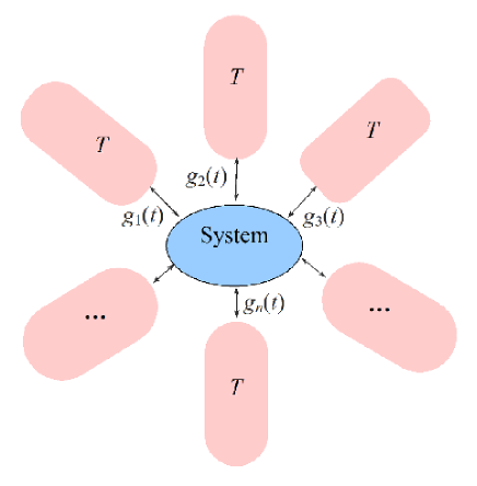
Figure 2: A schematic representation of the generalized model described in this work. The subsystem interacts with multiple bath reservoirs by means of time-dependent couplings while the temperature in each bath is also subject to change. (Color online.)

The target system is directly coupled to a large number of local reservoirs. These reservoirs are, in turn, coupled to a larger scale environment —to wit, the global environment— that alters its properties and interaction with the system over much longer time scales than the reservoir relaxation times. In principle, a detailed Hamiltonian can be written that would include the degrees of freedom for the system, the local environments and the global environment illustrated in Fig. 1. Given such a specification, a projection of the Hamiltonian to the system alone, and a study of its correlation functions would reveal its effective temperature and related properties. However, we found earlier that the projection onto a system coupled to a single time-dependent local reservoir can be described by the iGLE and an associated time-dependent Hamiltonian.Hernandez (1999); Vogt and Hernandez (2005) In what follows, we thus take a simpler approach to the solution of our objective by generalizing the iGLE and its associated time-dependent Hamiltonian for the case that the system can be coupled to many distinct local reservoirs. While much of the discussion takes advantage of the form of the auxiliary Hamiltonian system to derive various correlation functions, all of the latter involve only variables of the reduced dimensional system. As such, these results are independent of the particular specification of the auxiliary Hamiltonian.

II.1 Multiple-reservoir model with fixed temperature

The Brownian motion of a tagged —or chosen— particle immersed in a single equilibrium thermal bath is well understood. More generally, however, the local environment of the particle can be further divided into a set of different reservoirs —viz. distinct local baths— with separately identifiable characteristic properties. In this section, all of these reservoirs are assumed to be at the same temperature and therefore independently satisfy the same Boltzmann distribution over their coordinates, (c.f., Fig. 3).

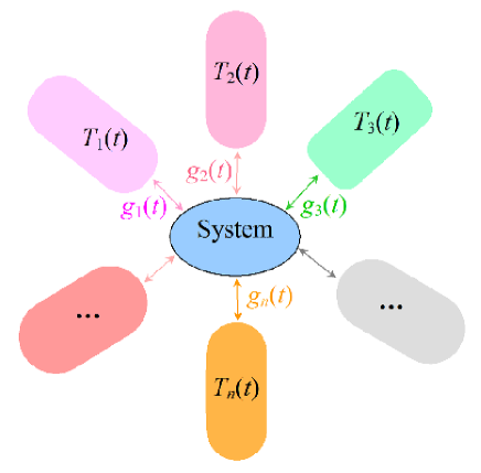
Figure 3: A schematic representation of the model investigated in Refs. Hernandez and Somer, 1999, Hernandez, 1999, and Popov et al., 2006. The subsystem interacts with multiple bath reservoirs by means of time-dependent couplings while the temperature remains constant. (Color online.)

A more general case in which these reservoirs may follow different temperatures —and consequently, as a whole, the environment does not follow a simple sing-temperature Boltzmann distribution— is addressed in the next section.

In order to describe the dynamics of a particle solvated by many distinct reservoirs, one can generalize slightly the Zwanzig-type Hamiltonian:Hernandez (1999); Popov et al. (2006)

$$H = \frac{p_{q}^{2}}{2}+V(q)+\delta V_{1}(q,t)+\delta V_{2}(q(\cdot),t)$$ (6)

$$-\sum_{k}g_{k}(t)\sum_{i}c^{(k)}_{i}x^{(k)}_{i}q+\sum_{k}H^{(k)}_{\rm b}\;,$$

where each reservoir, $k$, is represented by a distinct set of harmonic modes. The modes in each reservoir interact directly only with each other and the tagged particle, and indirectly to modes in other reservoirs through their mutual coupling to the tagged particle. In the Hamiltonian of Eq. (6), the sum of the first and second terms, $p_{q}^{2}/2+V(q)$, is the bare energy of the tagged particle. The last term is a sum of Hamiltonians,

$$H_{\rm b}^{(k)}=\frac{1}{2}\sum_{i}\left[\left(p^{(k)}_{i}\right)^{2}+\left(\omega_{i}^{(k)}x^{(k)}_{i}\right)^{2}\right]\;,$$ (7)

each of which represents the energy of the k-th bath reservoir with coordinates $x_{i}^{(k)}$ and momenta $p_{i}^{(k)}$. The fifth term provides the bilinear coupling between the bath modes and the particle, in which $\sum_{k}$ and $\sum_{i}$ denote the summation over the bath reservoirs and the bath modes (i.e., bath frequencies). The third term,

$$\delta V_{1}(q,t)=\frac{1}{2}\sum_{k}\sum_{i}g_{k}^{2}(t)\left(\frac{c^{(k)}_{i}}{\omega_{i}^{(k)}}\right)^{2}q^{2}\;,$$ (8)

is the renormalization of the potential which eliminates the time-dependent spectral shift, and the fourth term,

$$\delta V_{2}(q(\cdot),t)=\frac{1}{2}\int_{0}^{t}dt^{\prime}a(t,t^{\prime})[q(t^{\prime})-q(t)]^{2}-\frac{1}{2}q(t)^{2}\int_{0}^{t}dt^{\prime}a(t,t^{\prime})\;,$$ (9)

provides the time-dependent correction to the memory effects.Hernandez (1999); Popov et al. (2006) The nonstationary memory correction in Eq. (9) was defined earlier as

$$a(t,t^{\prime})=\sum_{k}g_{k}(t)\dot{g}_{k}(t^{\prime})\gamma_{{\rm(th)}k}(t-t^{\prime})\;,$$ (10)

where

$$\gamma_{{\rm(th)}k}(t-t^{\prime})=\sum_{i}\left(\frac{c^{(k)}_{i}}{\omega_{i}^{(k)}}\right)^{2}\cos\omega_{i}^{(k)}(t-t^{\prime})$$ (11)

is the friction kernel for the $k$-th reservoir at thermal equilibrium.

The nonlocality in the $\delta V_{2}(q(\cdot),t)$ term has been addressed earlierHernandez (1999); Popov et al. (2006) and is necessary because of the time dependence in the coupling terms. (If said time dependence were zero then this term would also be zero.) The former, in principle, also arises in the case of space-dependent frictionLindenberg and Seshadri (1981); Carmeli and Nitzan (1982, 1983); Lindenberg et al. (1983); Lindenberg and Cortés (1984) —viz. space-dependent coupling— where the factors $g_{k}$ in the fifth term of Eq. (6) depend only on the coordinate $q$. Although the transient coupling terms have recently been noted in said case,Jayannavar and Mahato (1995); Mahato et al. (1996) they have been completely discarded in the corresponding Hamiltonian equations of motion by way of heuristic arguments concerned with the possibility that they appear to violate causality. In the present case, however, where several coupling terms depend explicitly on time, the nonstationary memory correction $\delta V_{2}(q(\cdot),t)$ —requiring the integration over the particle’s path $q(\cdot)$ over all time— cannot be discarded. Indeed, this correction is necessary so as to ensure that the projection onto the iGLE does not itself contain additional nontrivial terms as detailed in Appendix B that would violate causality. As detailed earlier the component of the nonstationary memory correction that violates causality does not present any problems because it is smaller than other terms that have also been neglected in this formalism.

In Ref. Hernandez, 1999, the iGLE —Eq. (3)— (with a family of nonstationary friction kernels) was shown to be the projection of the equations of motion derived from Hamiltonian (6) when there is only one reservoir. In the current case of multiple reservoirs, the friction kernel in the iGLE can be represented as a sum of equilibrium friction kernels modulated by distinct functions $g_{k}(t)$ defining the coupling strength to the corresponding bath reservoirs,

$$\gamma(t,t^{\prime})=\sum_{k}g_{k}(t)g_{k}(t^{\prime})\gamma_{{\rm(th)}k}(t-t^{\prime})\;.$$ (12)

The functions $g_{k}(t)$ are specified by the time-dependence of the coupling up to a trivial arbitrariness in their initial values that is renormalizable. In cases when the reservoir is initially uncoupled to the particle, then said values are necessarily specified and equal to zero, however.

The FDR (5) for the projection of the iGLE, Eq. (3), with the multi-reservoir friction, Eq. (12), results from the Hamiltonian of Eq. (6), if the initial distribution is of the form,

$$P \propto \exp\left[-\frac{1}{2k_{\rm B}T}\sum_{k,i}\left(\left[p^{(k)}_{i}(0)\right]^{2}\right.\right.$$ (13)

$$\left.\left.+\left[\omega_{i}^{(k)}x^{(k)}_{i}(0)-\frac{c^{(k)}_{i}g_{k}(0)}{\omega_{i}^{(k)}}q(0)\right]^{2}\right)\right]\;,$$

and the conditions

$$\left<p^{(k)}_{i}(0)p^{(l)}_{j}(0)\right>=k_{\rm B}T\delta_{ij}\delta_{kl}\;,$$ (14a)

$$\left<\left(\omega_{i}^{(k)}x^{(k)}_{i}(0)-\frac{c^{(k)}_{i}g_{k}(0)}{\omega_{i}^{(k)}}q(0)\right)\right.$$

$$\left.\times\left(\omega_{j}^{(l)}x^{(l)}_{j}(0)-\frac{c^{(l)}_{j}g_{l}(0)}{\omega_{j}^{(l)}}q(0)\right)\right>$$

$$=k_{\rm B}T\delta_{ij}\delta_{kl}\;,$$ (14b)

$$\left<p^{(k)}_{i}(0)\left(\omega_{j}^{(l)}x^{(l)}_{j}(0)-\frac{c^{(l)}_{j}g_{l}(0)}{\omega_{j}^{(l)}}q(0)\right)\right>$$

$$=0$$ (14c)

are satisfied.

The iGLE with multiple and distinct reservoirs has thus been specified, and allows for temporal changes in the response of the environment albeit while all such reservoirs maintain the same constant temperature.

II.2 Multiple-reservoir model with time-dependent response

II.2.1 Squeezing bath modes

In principle, the effective temperature of each of the reservoirs (solvating the tagged particle) need not be the same as they are not coupled to each other directly. This situation is illustrated in Fig. 2 in which the temperature of each reservoir is different, perhaps as a consequence of some unspecified external or internal processes. It can be implemented within the Hamiltonian representation of a particle interacting with multiple reservoirs by supposing that the bath modes are not static—that is, their effective masses and coordinate scales are allowed to vary in time.

The time-dependent functions, $h_{k}(t)$ and $\mu_{k}(t)$, are now introduced so as to represent the time-dependent scaling in the force constant and mass of the $k^{\rm th}$ bath mode, respectively. The Hamiltonian of the $i$-th oscillatory bath mode belonging to the $k$-th reservoir can thereby be written as

$$H^{(k)}_{{\rm b},i}(x^{(k)}_{i},p^{(k)}_{i},t)=\frac{\left[p^{(k)}_{i}\right]^{2}}{2\mu_{k}^{2}(t)}+\frac{1}{2}\left[\omega_{i}^{(k)}h_{k}(t)x^{(k)}_{i}\right]^{2}\;.$$ (15)

The terms, $h_{k}(t)$ and $\mu_{k}(t)$, combine to determine the time dependence of the mode frequencies in the k-th reservoir. Their initial values can be chosen as $h_{k}(0)=\mu_{k}(0)=1$ without loss of generality. Meanwhile, the scaling of the force constant effectively narrows (or widens) the configuration space available to the oscillator at a given temperature. Such a trick of “squeezing” bath oscillators leads to changes in the total energy of the reservoir, and thereby shifts the reservoir temperature. The existence of such temperatures relies on the fact that the relaxational redistribution of the collective energy within the modes is sufficiently fast that bath reequilibrates on the time scales of the particle motion. In other words, the process of bath mode squeezing is assumed to be adiabatic and to vary on time scales longer than the periods of oscillation in the nontrivial modes of a given reservoir.

The time-dependent Hamiltonian (6) can now be modified by introducing the scaling functions $h_{k}(t)$ and $\mu_{k}(t)$:

$$H = \frac{p_{q}^{2}}{2}+V(q)+\delta V_{1}(q,t)+\delta V_{2}(q(\cdot),t)$$

$$- \sum_{k,i}c^{(k)}_{i}g^{\prime}_{k}(t)h_{k}(t)x^{(k)}_{i}q+\sum_{k,i}H^{(k)}_{{\rm b},i}(x^{(k)}_{i},p^{(k)}_{i},t)\;.$$

Here the coupling coefficients $g^{\prime}_{k}(t)$ are introduced so as to simplify the structure of the Hamiltonian. These coefficients are unequal to the earlier coefficients $g_{k}(t)$. Nevertheless they can be connected through the expression,

$$g^{\prime}_{k}(t)=g_{k}(t)\sqrt{\frac{h_{k}(t)}{\mu_{k}(t)}}\;,$$ (17)

allowing comparison to the earlier results obtained using the original iGLE.Hernandez and Somer (1999); Somer and Hernandez (1999); Hernandez (1999); Popov et al. (2006) In Eq. (II.2.1) the renormalization potential, $\delta V_{1}$, is given by Eq. (8) with $g_{k}(t)$ replaced by $g^{\prime}_{k}(t)$. The nonstationary memory correction, $\delta V_{2}$, is defined by Eq. (9) with

$$a(t,t^{\prime})=\sum_{k}\frac{h_{k}(t)}{\mu_{k}(t)}g_{k}(t)\dot{g}_{k}(t^{\prime})\gamma_{{\rm(th)}k}\left[\tau_{k}(t)-\tau_{k}(t^{\prime})\right]\;,$$ (18a)

where $$g_{k}(t) g^{\prime}_{k}(t)$$ has not been replaced by ,

$$\tau_{k}(t)\equiv\int_{0}^{t}h_{k}(s)/\mu_{k}(s)ds$$ (18b)

and $$\gamma_{{\rm(th)}k}(\cdot)$$ is defined in Eq. (11).

Note that the coupling coefficients $g_{k}(t)$ can also depend on the temperature. Although in the framework of this approach, there is no recipe for connecting the temperature-driving functions $\mu_{k}(t)$ and $h_{k}(t)$ to these coefficients, such a connection can in principle be obtained from a deeper analysis based on mode-coupling theory, direct extraction of these functions from simulations (Ref. Popov et al., 2006; see also Sec. III.3 below), or experiments.

As was done in the earlier section with respect to the behavior of $g_{k}(t)$, the functions $\mu_{k}(t)$ and $h_{k}(t)$ must be required to be effectively stationary on the correlation time scales of the fastest bath modes.Millonas and Ray (1995); Chaudhuri et al. (1998) This so-called slow-bath-mode “squeezing” assumption is necessary because otherwise there would always exist a bath mode whose response to fluctuations would be so chaotic that it wouldn’t ever relax to quasi-equilibrium limits. Evidently, for low spectral frequencies, this imposes some restrictions on the rates of change of $\mu_{k}(t)$ and $h_{k}(t)$ and, thus, implies a related assumption that low frequency bath modes contribute negligibly to the particle’s motion. These assumptions are valid, for example, in the over-damped case when the spectral density, $J(\omega)$, of the bath Hamiltonian is proportional to $\omega^{s}$ with $s>1$ at $\omega\rightarrow 0$, and hence the small bath frequencies are not coupled to the system.

II.2.2 The effective temperature of each reservoir

The strategy for solving the dynamics of Eq. (15), taking into account its hierarchical structure, focuses first on the solution of the local dynamics of the bath modes within a given $k^{\rm th}$ reservoir as if it does not interact with the rest of the modes. In the next section, we will use these states as a reference for the approximate solution of the global dynamics. The accuracy of this approach relies on the assumption that the coupling between the reservoirs and the tagged particle is weak, as has indeed been assumed from the outset. For simplicity, in this subsection the upper indices $(k)$ will often be omitted as all of the formulas herein are necessarily being solved within a given $k^{\rm th}$ reservoir.

At any given time, the energy manifold of the $i^{\rm th}$ bath mode in the $k^{\rm th}$ reservoir is simply a function of the phase space variables, $(x_{i},p_{i})$, determined by the instantaneous parameters, i.e.,

$$E_{i}(t)=\frac{p_{i}^{2}}{2\mu_{k}^{2}(t)}+\frac{\omega_{i}^{2}}{2}h_{k}(t)^{2}x_{i}^{2}\;.$$ (19)

If $\mu_{k}(t)$ and $h_{k}(t)$ change slowly relative to the oscillator frequency, then the symplectic area of this manifold —viz., the action $I$— will be an adiabatic invariant. On the elliptical energy manifold defined by Eq. (19), this invariant is given by

$$I=\frac{\mu_{k}(t)E_{i}(t)}{h_{k}(t)\omega_{i}}=\frac{\mu_{k}(0)E_{i}(0)}{h_{k}(0)\omega_{i}}=\frac{E_{i}(0)}{\omega_{i}}\;,$$ (20)

where the last equality follows from the initial choice, $h_{k}(0)=\mu_{k}(0)=1$. The time-invariance of $I$ thus provides a useful connection,

$$E_{i}(t)=E_{i}(0)\frac{h_{k}(t)}{\mu_{k}(t)}\;,$$ (21)

between the energies of the $i^{\rm th}$ bath mode at various times.

Given that each bath mode is initially equilibrated at its corresponding reservoir temperature $T_{k}(0)$ —i.e., the initial energies $E_{i}(0)$ of the reservoir are Boltzmann distributed,— the connection in Eq. (21) readily implies that the energies $E_{i}(t)$ at any given time are also Boltzmann distributed at the temperature,

$$T_{k}(t)=T_{k}(0)\frac{h_{k}(t)}{\mu_{k}(t)}\;.$$ (22)

Thus, the ratio $h_{k}(t)/\mu_{k}(t)$ establishes the time dependence in the temperature of the $k^{\rm th}$ bath reservoir. Although the interaction between the reservoir and the tagged particle could, in principle, alter this structure by way of heat transfers, in practice it does not do so. The bath reservoir is assumed to be sufficiently large that such transfers are small in comparison with the total energy of the reservoir. (This assumption is not very severe because it must be satisfied in order for the bath to have a well-defined quasi-equilibrium temperature!) The functions $h_{k}(t)$ and $\mu_{k}(t)$ are auxiliary and are not known a priori, but the time-dependent temperature entering in Eq. (22), together with the coupling strength coefficients $g_{k}(t)$, can either be found from simulations or estimated from experimental data. For example, they have been obtained in the case of a diffusing particle in a swelling colloidal suspension in Ref. Popov et al., 2006.

The initial temperatures of the various bath reservoirs need not be the same because some modes may be connected to distinct heat sources and sinks leading to steady state energy transport through the system between the reservoirs. Indeed, the nonequilibrium dynamics of a particle connected to reservoirs with different time-independent temperatures has been explored by Kurchan and coworkers.Cugliandolo and Kurchan (2000); Zamponi et al. (2005) But if the system is initially in equilibrium, then in the absence of such energy flows, the initial temperatures of all the reservoirs will be the same. More generally, however, the initial probability distributions —cf. Eq. (13)— for a given reservoir can be rewritten as,

$$P_{k} \propto \exp\left\{-\sum_{i}\frac{1}{2k_{\rm B}T_{k}(0)}\left(\left[p^{(k)}_{i}(0)\right]^{2}\right.\right.$$ (23)

$$\left.\left.+\left[\omega_{i}^{(k)}x^{(k)}_{i}(0)-\frac{c^{(k)}_{i}g_{k}(0)}{\omega_{i}^{(k)}}q(0)\right]^{2}\right)\right\}\;,$$

for the $k^{\rm th}$ reservoir temperature, $T_{k}(0)$. The correlations in Eqs. (14a)-(14) are still satisfied if one replaces the temperature, $T$ with that of the given reservoir, $T_{k}(0)$. Such an initial equilibration seems to be artificial when the temperatures $T_{k}$ change with time due to the interactions of reservoirs with the tagged subsystem and the global bath. Note, however, that the initial time, $t=0$, can be formally shifted to the far past. The system then has no memory of the initial conditions and, thus, the resulting iGLE remains unaffected.

II.2.3 Equations of motion

The equations of motion for the many-reservoir case follows directly from the Hamiltonian in Eq. (II.2.1):

$$\dot{x}_{i}^{(k)} = \frac{p_{i}^{(k)}}{\mu_{k}^{2}(t)}\;,$$ (24a)

$$\dot{p}_{i}^{(k)} = -\left[h_{k}(t)\omega_{i}^{(k)}\right]^{2}x_{i}^{(k)}+c_{i}g^{\prime}_{k}(t)h_{k}(t)q\;,$$ (24b)

$$\dot{q} = p_{q}\;,$$ (24c)

$$\dot{p}_{q} = -\frac{\partial V(q)}{\partial q}+\sum_{k,i}c_{i}^{(k)}g^{\prime}_{k}(t)h_{k}(t)x_{i}^{(k)}$$

$$-\sum_{k,i}\left(\frac{c_{i}^{(k)}g^{\prime}_{k}(t)}{\omega_{i}^{(k)}}\right)^{2}q-\frac{\partial}{\partial q(t)}\delta V_{2}(q(\cdot),t)\;,$$

where the indices, $k$, referring to a given reservoir have been explicitly retained to help the reader. However, they are somewhat cumbersome, and so in this section it is convenient to replace explicit reference to the superscripted reservoir index. Instead the collective index ${\bf i}(\equiv\{i,k\})$ will be used for this reference, as in e.g. $\omega_{\bf i}\equiv\omega_{i}^{(k)}$.

As discussed in Sec. II.1, the presence of the nonstationary memory correction $\partial(\delta V_{2})/\partial q(t)$ in Eq. (24) introduces the possibility of violations of the causality principal. Indeed, the variational principle applied to the calculation of this term gives an apparent contribution to the force from future trajectories. However the error in this contribution is on the order of the neglected terms in the perturbative treatment in the projection, and it was seen earlier Popov et al. (2006) that all of these small errors can be safely neglected. But the nonstationary memory correction $\partial(\delta V_{2})/\partial q(t)$ can not be entirely neglected because it contains a nontrivial correction which ensures that the projection to the iGLE does not violate causality up to the second order of the perturbation expansion (c.f., Appendix B).

From Eqs.(24a) and (24b) one can derive

$$\ddot{x}_{\bf i}+\nu_{k}(t)\dot{x}_{\bf i}+\Omega^{2}_{\bf i}(t)x_{\bf i}=c_{\bf i}\frac{g^{\prime}_{k}(t)h_{k}(t)}{\mu_{k}^{2}(t)}q\;,$$ (25)

where

$$\nu_{k}(t) = \frac{2\dot{\mu}_{k}(t)}{\mu_{k}(t)}\;,$$ (26a)

$$\Omega_{\bf i}(t) = \frac{h_{k}(t)}{\mu_{k}(t)}\omega_{\bf i}\;.$$ (26b)

The assumption of a slow“squeezing” bath modes, discussed before, must now be restated in terms of both time dependent parameters, $h_{k}(t)$ and $\mu_{k}(t)$. After a little algebra, it can be shown to reduce to the requirement

$$\left|\frac{\dot{\mu}_{k}}{\mu_{k}}+\frac{\dot{h}_{k}}{h_{k}}\right|\ll\Omega_{\bf i}\;,$$ (27)

which must be satisfied for all modes $i$ in a $k^{\rm th}$ reservoir. Under this assumption, one obtains the following result [as is shown in Appendix A)]:

$$x_{\bf i} = u_{\bf i}(t)x_{\bf i}(0)+u_{\bf i}(t)\dot{x}_{\bf i}(0)\int_{0}^{t}\frac{dt^{\prime}}{(u_{\bf i}(t^{\prime})\mu_{k}(t^{\prime}))^{2}}$$

$$+ c_{\bf i}u_{\bf i}(t)\int_{0}^{t}\frac{dt^{\prime}}{(u_{\bf i}(t^{\prime})\mu_{k}(t^{\prime}))^{2}}\int_{0}^{t^{\prime}}{g^{\prime}_{k}(s)h_{k}(s)u_{\bf i}(s)q(s)ds}\;,$$

where the bath mode oscillations are described by

$$u_{\bf i}(t)=\frac{\cos\omega_{\bf i}\tau_{k}(t)}{\sqrt{\mu_{k}(t)h_{k}(t)}}\;,$$ (29)

and the effective time $\tau_{k}$ can be written as

$$\tau_{k}(t)\equiv\frac{1}{\omega_{\bf i}}\int_{0}^{t}{\Omega_{\bf i}(t^{\prime})dt^{\prime}}=\int_{0}^{t}{\frac{h_{k}(t^{\prime})}{\mu_{k}(t^{\prime})}dt^{\prime}}=\int_{0}^{t}{\frac{T_{k}(t^{\prime})}{T_{k}(0)}dt^{\prime}}\;.$$ (30)

Perhaps not surprisingly, the effective time changes “faster” when the temperature increases. A similar transformation of time has been found earlier in simplifying overdamped Langevin equations driven by time-dependent temperature baths. Reimann (2002); Hänggi (1981); Reimann et al. (1996)

The projected equation of motion for the tagged particle reduces to the iGLE form after the appropriate averaging over the distributions derived in the previous subsection. (The details of this derivation can be found in Appendix B.) The nonstationary friction has a form similar to that of Eq. (3) with

$$\gamma(t,t^{\prime}) = \sum_{k}\frac{T_{k}(t)}{T_{k}(0)}g_{k}(t)g_{k}(t^{\prime})\gamma_{{\rm(th)}k}(\tau_{k}(t)-\tau_{k}(t^{\prime}))$$ (31a)

$$= \sum_{k}\sqrt{\frac{T_{k}(t)}{T_{k}(t^{\prime})}}\gamma_{k}(t,t^{\prime})$$ (31b)

for $$t>t^{\prime} k^{\rm th}$$, where the weighted friction of the mode is defined as

$$\gamma_{k}(t,t^{\prime})\equiv\frac{\sqrt{T_{k}(t)T_{k}(t^{\prime})}}{T_{k}(0)}g_{k}(t)g_{k}(t^{\prime})\gamma_{{\rm(th)}k}(\tau_{k}(t)-\tau_{k}(t^{\prime}))\;,$$ (31c)

and is symmetric in the two times, $t$ and $t^{\prime}$. (Note that $\gamma_{{\rm(th)}k}(\cdot)$ is an even function of its argument as can be seen in Eq. (11).) Recalling the definition for the bath reservoir temperature and friction kernel in Eqs. (22), and Eq. (11), respectively, the nonstationary stochastic force is found to be

$$\xi(t) = \sum_{k}\frac{T_{k}(t)}{T_{k}(0)}g_{k}(t)\sum_{i}\frac{c_{\bf i}}{\omega_{\bf i}}$$ (32)

$$\times\left[p_{\bf i}(0)\sin\omega_{\bf i}\tau_{k}(t)+\left(\omega_{\bf i}x_{\bf i}(0)-\frac{c_{\bf i}g_{k}(0)}{\omega_{\bf i}}q(0)\right)\cos\omega_{\bf i}\tau_{k}(t)\right]\;.$$

Imposing the initial condition in Eq. (23), the random force correlation function becomes

$$\left<\xi(t)\xi(t^{\prime})\right> = \sum_{k}k_{\rm B}\frac{T_{k}(t)T_{k}(t^{\prime})}{T_{k}(0)}g_{k}(t)g_{k}(t^{\prime})\gamma_{{\rm(th)}k}(\tau_{k}(t)-\tau_{k}(t^{\prime}))$$ (33a)

$$= k_{\rm B}\sum_{k}\sqrt{T_{k}(t)T_{k}(t^{\prime})}\gamma_{k}(t,t^{\prime})\;.$$ (33b)

Equations (31) and (33) can be used to recast the extended form of the FDR,

$$\left<\xi(t)\xi(t^{\prime})\right>=k_{\rm B}T_{\rm eff}(t,t^{\prime})\gamma(t,t^{\prime})\;,$$ (34a)

where the effective temperature is

$$T_{\rm eff}(t,t^{\prime})=\frac{\sum_{k}\sqrt{T_{k}(t)T_{k}(t^{\prime})}\gamma_{k}(t,t^{\prime})}{\sum_{k}\sqrt{\frac{T_{k}(t)}{T_{k}(t^{\prime})}}\gamma_{k}(t,t^{\prime})}\;,$$ (34b)

for $t>t^{\prime}$. Eqs. (34) comprise the central result of this work and generalize the FDR by including the simultaneous interactions of the tagged particle with different nonstationary thermal reservoirs. In particular Eq. (34b) provides a clear prescription of the effective temperature of the chosen particle that emerges as a consequence of averaging the microscopic dynamics of many reservoirs. This is a nontrivial result because it dances between microscopic and macroscopic quantities. Moreover, as written, the effective temperature appears to be asymmetric between the two times, $t$ and $t^{\prime}$, and hence may cause alarm. However, only the product $T_{\rm eff}$ and $\gamma$ in Eq. (34a) must remain symmetric. As shown in the discussion that follows, this product is indeed symmetric with respect to the two times in its argument, and $T_{\rm eff}$ reduces to forms that have earlier been derived or assumed for a number of limiting cases.

One possible concern with the underlying equations that have led to the Eq. (34) lies in the specification of the initial condition for the system and its environment, given that there must evidently be some environmental memory of the previous motion by way of the values of $q(t)$ at earlier times. In past and present work, we have typically employed one of three boundary conditions: (i) The system is at equilibrium at the initial time, 0, just before the nonequilibrium disturbance is effected. This requires us to run dynamics starting at a time well prior to $t=0$ allowing the system to equilibrate and fully prepare its environmental memory. (This evidently requires sampling over many trajectories.) (ii) Different reservoirs at $t=0$ are at distinct equilibrium within themselves, but are not at equilibrium with each other. In this case, we prepare each reservoir separately using the procedure described for case i. (iii) The particle is suddenly placed inside the reservoirs, and hence there is no prior memory due to motion before $t=0$. In this section, we have applied the boundary conditions from case ii, in order to simplify the expressions from correction terms that would have been trivial anyway. Indeed, the use of case iii for the boundary conditions in the numerical simulations shown below did not affect the results.

It may appear that the terms in the central result of Eq. (34) are contingent on the creation of an associated Hamiltonian of the form of Eq. (15) used in its analytical derivation. However, as in other such reconstructions using the latter auxiliary infinite-dimensional representation, the projected form of the central result contains no object with explicit reference to any unprojected dynamics. As such, it should be capable of describing any dynamics which is captured by the continuum representation of the iGLE. More specifically, the temperatures $T_{k}$ can be calculated or measured directly from each of the independent baths. The coupling terms $g_{k}$ and memory times $\tau_{k}$ can be calculated or measured directly by obtaining the correlation functions of the forces exerted on the tagged particle by each bath, respectively, upon removal of the thermal component. Such a procedure has been used in Ref. Popov et al., 2006 in the limit in which the chosen particle is coupled to only one bath. Several additional examples are provided below in which the particle is coupled to multiple baths. In each of these cases, the associated functions, $g_{k}(t)$, $\tau_{k}(t)$, and $T_{k}(t)$, necessary for the application of Eq. (34) are constructed. It is notable, that these functions can be obtained without recourse to the auxiliary infinite-dimensional form of Eq. (15).

III Results and Discussion of Limiting Cases

In order to better understand the effective temperature expression derived above, it is helpful to look at a number of limiting cases. In Sec. III.1, the structure of the correlation functions when all the reservoirs are held at constant but distinct temperatures is shown to agree with the earlier perspective of Kurchan and coworkers.Zamponi et al. (2005) In Sec. III.2, the generalized Langevin equations used earlier to describe aging systems are recovered for when the reservoirs are all held at a homogeneous, but time-dependent, temperature. This latter limit is also equivalent to that suggested earlier in Ref. Popov et al., 2006 in a case studying driven nonequilibrium colloidal suspensions. In Sec. III.3.2, the two-temperature model of Refs. Millonas and Ray, 1995 and Chaudhuri et al., 1998 is also recovered in the limit that the system is coupled to two local reservoirs. A set of gedenken experiments wherein the bath is coupled to three local reservoirs is shown in Sec. III.3.3 to lead to a nontrivial effective temperature in agreement with the central results of this work. In Sec. III.3.4, the local quasi equilibrium limit of a non-Markovian Fokker-Planck equation explored earlier by Rubi and coworkersSantamaria-Holek et al. (2004) is shown to lead to correlation functions equivalent to those in the corresponding limit of this work. Thus the central result for the effective temperature of the system driven by nonequilibrium local environments is shown to capture all the previous limits as well as extend the formalism to heretofore unknown cases.

Before proceeding, it is perhaps also useful to recapitulate the separation of time scales in the hierarchy illustrated by Fig. 1 that has been assumed in constructing the central result in Eq. (34). The relaxation times for responses to large perturbations of the system $\tau_{\rm s}$, the local reservoirs $\tau_{k}$, and the global environment $\tau_{\rm g}$ must satisfy the simple ordering, $\tau_{\rm s}\leq\tau_{k}\leq\tau_{\rm g}$. Meanwhile, the system is so small compared to the local reservoir that any perturbation at times on the order of $\tau_{\rm s}$ leads to no effective change of the local reservoir behavior. Any sustained change in the system behavior over times longer than $\tau_{k^{{}^{\prime}}}$ will affect and change the behavior of the ${k^{{}^{\prime}}}^{\rm th}$ reservoir, but it will simply lead to a change of the quasi-static response of said reservoir to the system at the short times scales near $\tau_{\rm s}$. An analogous description is true for the time scales between the local reservoirs and the global bath. Because of these inequalities, any time-dependence in $T_{k}$ and $g_{k}$ must be slow in comparison with the motion of the system. However, as we have seen in earlier work, and shown here in the numerical work, the time scales do not have to be nearly so disparate as the corrections are small.

III.1 Environments with Constant Temperature Inhomogeneities

The structure of Eq. (33) and the associated stochastic equations derived from them allows one to describe the dynamics of a chosen particle connected to many reservoirs where each can be at a different temperature. If these temperatures are constant in time, i.e., $T_{k}(t)=T_{k}(t^{\prime})=T_{k}$, then from Eqs. (30), (31a) and (33) one obtains

$$\gamma(t,t^{\prime}) = \sum_{k}g_{k}(t)g_{k}(t^{\prime})\gamma_{{\rm(th)}k}(t-t^{\prime})\;,$$ (35)

$$\left<\xi(t)\xi(t^{\prime})\right> = \sum_{k}k_{\rm B}T_{k}g_{k}(t)g_{k}(t^{\prime})\gamma_{{\rm(th)}k}(t-t^{\prime})\;.$$ (36)

An analogous case has been discussed in Ref. Zamponi et al., 2005 in the stationary limit when $g_{k}(t)\equiv 1$ (stable non-uniform environment). Thus, Eqs. (35) and (36) extend the previous treatment so as to include nonequilibrium baths.

The implementation of the iGLE theoretical framework discussed above follows readily for any given nonequilibrium system interacting with many nonequilibrium baths. The key step is the identification of which baths —viz., temperature heat sinks— are in contact with the chosen particle as a function of time. Nonzero and zero values of $g_{k}(t)$ at any given time correspond to whether said reservoir is connected and disconnected, respectively, from the particle at the given time, $t$. (An analogous procedure was used in Ref. Jarzynski, 2000 for deriving a variant of the fluctuation theorem.) This will help to switch the chosen subsystem between different heat reservoirs with different temperatures. If the reservoir temperature does not change significantly during a period when an appropriate coupling term differs from zero, one obtains Eqs. (35) and (36).

III.2 Environments with Time-Dependent Homogeneous Temperature

If the temperature changes uniformly for all the bath modes, $T_{k}(t)=T(t)$, then Eq. (33) simplifies to

$$\left<\xi(t)\xi(t^{\prime})\right>=k_{\rm B}T(t^{\prime})\gamma(t,t^{\prime})\;.$$ (37)

Such generalized FDRs (GFDRs) have been used in the description of the nonequilibrium steady-state dynamics of glassy systems, for example.Crisanti and Ritort (2003); Frey and Kroy (2005) The relations between autocorrelation and response functions, like that of Eq. (37), are frequently considered in the literature as a signature of FDR violations (quasi-FDR) arising from partial equilibration among a subset of degrees of freedom, and the quantity $T(t^{\prime})$ is treated as an effective temperature. In the specific case of aging systems,Crisanti and Ritort (2003); Sollich et al. (2002); Fielding and Sollich (2002) the effective temperature depends on both $t$ and $t^{\prime}$. The name “quasi-FDR” and the use of $T_{\rm eff}$ as an auxiliary parameter are reasonable due to the fact that the actual thermodynamic temperature is constant in these studies.

The results of the previous section, however, allow for the recognition that $T(t^{\prime})$ is the true ambient temperature at the time $t^{\prime}$, and the interpretation that GFDR in Eq. (37) expresses the transient behavior of the system. Note, that in the iGLE model, the partial relaxation of the baths corresponds to different dependencies $T_{k}(t)$ [included into the GFDR, Eq. (33)], and leads to the two-time dependence of $T_{\rm eff}$ in Eq. (34a).

In the specific case when all the coupling coefficients are also equal, $g_{k}(t)=g(t)$, we obtain

$$\gamma(t,t^{\prime})=\frac{T(t)}{T(0)}g(t)g(t^{\prime})\gamma_{\rm th}(\tau(t)-\tau(t^{\prime}))\;,$$ (38)

for $t>t^{\prime}$, where $\gamma_{\rm th}(\tau-\tau^{\prime})\equiv\sum_{k}\gamma_{{\rm(th)}k}(\tau-\tau^{\prime})$ is the friction kernel of the whole system at equilibrium, and

$$\xi(t)=\frac{T(t)}{T(0)}g(t)\xi_{\rm th}(\tau(t))\;,$$ (39a)

with

$$\left<\xi_{\rm th}(\tau)\xi_{\rm th}(\tau^{\prime})\right>=k_{\rm B}T(0)\gamma_{\rm th}(\tau-\tau^{\prime})\;.$$ (39b)

It is instructive to compare these results with those obtained in Ref. Somer and Hernandez, 1999 from phenomenological considerations. Namely, the friction kernel used in that work,

$$\gamma(t,t^{\prime})=g(t)g(t^{\prime})\gamma_{\rm th}(t-t^{\prime})\;,$$ (40)

coincides with Eq. (4) and may include effects due to the temperature change implicitly through the coupling coefficient $g(t)$ only.

This restriction on the memory kernel also induces the main difference between the two approaches: the use of the real time $t$ vs. the effective one, $\tau(t)$. Hence, only the amplitude of the stochastic force changes along with the temperature alteration, and gives

$$\xi(t)=\sqrt{\frac{T(t)}{T(0)}}g(t)\xi_{\rm th}(t)\;.$$ (41)

The use of the real time instead of the parameterized one implies that the random force autocorrelation function acquires a different form:

$$\left<\xi(t)\xi(t^{\prime})\right>=k_{\rm B}\sqrt{T(t)T(t^{\prime})}g(t)g(t^{\prime})\gamma_{\rm th}(t-t^{\prime})=k_{\rm B}\sqrt{T(t)T(t^{\prime})}\gamma(t,t^{\prime})\;.$$ (42)

This FDR varies from Eq. (37) insignificantly if the temperature changes slowly during the solvent response time, when $\gamma_{\rm th}(t-t^{\prime})$ differs from zero. However, the use of the effective time to describe the behavior of the Gaussian noise in Eq. (39) provides an important contribution that allows the correct projected equations of motion to better control the intensity of the stochastic force when the bath is far from equilibrium. This is the main difference between the Hamiltonian approach of the current work and that of Ref. Somer and Hernandez, 1999 where the random force is governed only by the changing amplitude.

III.3 Stochastic Dynamics

The friction kernel of a free heavy particle, diffusing in solution without external potentials ($V(q)=0$), has a memory-less form,Kneller and Sutmann (2004)

$$\gamma_{({\rm th})k}(\tau)=2\gamma_{0k}\delta(\tau)\;.$$ (43)

Recalling the standard functional relation, $\delta(f(x))=\delta(x-x_{0})/|f^{\prime}(x_{0})|\;,$ where for simplicity we have assumed that $x_{0}$ is the only root of the argument, i.e. $f(x_{0})=0$, then Eqs. (31a) and (33) lead to

$$\gamma(t,t^{\prime}) = \sum_{k}g_{k}^{2}(t)\cdot 2\gamma_{0k}\delta(t-t^{\prime})\equiv 2\eta(t)\delta(t-t^{\prime})\;,$$ (44)

$$\left<\xi(t)\xi(t^{\prime})\right> = k_{\rm B}\sum_{k}T_{k}(t)g_{k}^{2}(t)\cdot 2\gamma_{0k}\delta(t-t^{\prime})\equiv k_{\rm B}T_{\rm eff}(t)\gamma(t,t^{\prime})\;,$$ (45)

where the effective temperature, $T_{\rm eff}(t)$, of the Brownian particle is set to

$$T_{\rm eff}(t)=\frac{\sum_{k}T_{k}(t)g_{k}^{2}(t)\gamma_{0k}}{\sum_{k}g_{k}^{2}(t)\gamma_{0k}}\;,$$ (46)

so as to satisfy the FDR.

The effective temperature is consistent with that of Refs. Cugliandolo and Kurchan, 2000 and Zamponi et al., 2005 for the special case when the noise is memoryless and all the reservoirs are stable in time —i.e., when the temperatures $T_{k}$ are constant and $g_{k}=1$. Herein, the resulting iGLE turns into the memoryless irreversible Langevin equation (iLE):

$$\ddot{q}(t) = -\eta(t)\dot{q}(t)+\xi(t)\;,$$ (47a)

$$\left<\xi(t)\xi(t^{\prime})\right> = 2k_{\rm B}T_{\rm eff}(t)\eta(t)\delta(t-t^{\prime})\;.$$ (47b)

The form of this stochastic equation of motion is similar to that of a particle diffusing in a medium with spatial temperature gradients: Mahato et al. (1996)

$$\ddot{q} = -\eta(q)\dot{q}+\xi(q,t)\;,$$ (48a)

$$\langle\xi(q,t)\xi(q,t^{\prime})\rangle = 2k_{\rm B}T(q)\eta(q)\delta(t-t^{\prime})\;.$$ (48b)

In both cases, the particle quickly equilibrates as it traverses from one local region to another, in conformity with the memoryless limit. Such a traversal is reminiscent of space-dependent friction dynamics wherein the stochastic particle traverses between distinct dissipating environments. The difference here is that the dissipation can change even if the particles stays in the same region because of changes in the dissipating environment. Thus the earlier Darboux-like topological construction of the dissipating environments is now extended to be time-dependent.

III.3.1 Uniform temperature Limit

In the limit that all the reservoirs obey a homogeneous temperature profile, $T_{k}(t)=T(t)$ for all $k$, so that $T_{\rm eff}(t)=T(t)$ (see Eq. (46)), the friction coefficient in Eq. (47) becomes

$$\eta(t)=G^{2}(t)\gamma_{0}\;,$$ (49)

where $G(t)$ is the effective coupling coefficient defined according to Ref. Popov et al., 2006,

$$G^{2}(t)=\sum_{k}\left.g^{2}_{k}(t)\gamma_{0k}\right/\gamma_{0}\quad\mbox{and}\quad\gamma_{0}=\sum_{k}\gamma_{0k}\,.$$ (50)

We thus recover the iGLE of Ref. Popov et al., 2006 in which the stochastic particle is effectively coupled to a single homogeneous (but time-dependent) reservoir.

III.3.2 Two-Reservoir Limit

In Refs. Millonas and Ray, 1995 and Chaudhuri et al., 1998, the LE for the Brownian particle is derived in the case that the latter is dissipated by two reservoirs: a global thermal bath at temperature $T$, and a local nonequilibrium (time-dependent) bath. The LE reads, as usual,

$$\ddot{q}(t)=-(\eta_{\rm eq}+\eta_{\rm neq})\dot{q}(t)+\xi(t)\;,$$ (51)

but with the stochastic force subdivided into equilibrium and nonequilibrium parts, $\xi(t)=\xi_{\rm eq}(t)+\xi_{\rm neq}(t)$. The FDR for the equilibrium part is $\langle\xi_{\rm eq}(t)\xi_{\rm eq}(t^{\prime})\rangle=2\eta_{\rm eq}k_{\rm B}T\delta(t-t^{\prime})$. The energy density of the nonequilibrium bath modes changes with time and was found in Refs. Millonas and Ray, 1995 and Chaudhuri et al., 1998 to be

$$u(\omega,t) = \frac{1}{4\eta_{\rm neq}}\int_{-\infty}^{\infty}d\tau\langle\xi_{\rm neq}(t)\xi_{\rm neq}(t+\tau)\rangle e^{i\omega\tau}$$ (52a)

$$= \frac{k_{\rm B}T}{2}+e^{-\nu t/2}\left[u(\omega,0)-\frac{k_{\rm B}T}{2}\right]$$ (52b)

This takes into account the average dissipation —$\nu$ in the notation of the earlier articles— of the nonequilibrium reservoir modes due to their coupling to the thermal reservoir.

Within the framework of the present approach, all the modes of the nonequilibrium reservoir have one and the same initial temperature, $u(\omega,0)=k_{\rm B}T_{0}/2$. The time-dependent temperature of this reservoir according to Eq. (52) is

$$T_{\rm neq}(t)=T+e^{-\nu t/2}(T_{0}-T)\;,$$ (53)

and it is the same for all the modes. Taking the inverse Fourier transform of Eq. (52), one obtains

$$\langle\xi(t)\xi(t+\tau)\rangle=2k_{\rm B}T_{\rm eff}(t)\eta\delta(\tau)\;,$$ (54)

where

$$T_{\rm eff}(t)=\frac{\eta_{\rm eq}T+\eta_{\rm neq}T_{\rm neq}(t)}{\eta_{\rm eq}+\eta_{\rm neq}}\,.$$ (55)

This latter result is in agreement with the effective temperature in Eq. (46) if $g_{k}(t)\equiv 1$. The latter requirement is precisely what is needed to ensure that all of the nonequilibrium baths reduce to the single local nonequilibrium bath under consideration in this subsection.

Hence the current construction of the generalized effective temperature of a particle connected to an arbitrary number of baths reduces to the appropriate limit when it is connected to two nearly-separable baths.

III.3.3 Three-Reservoir Gedenken Experiments

To further illustrate the accuracy of Eq. (46) in providing the effective temperature of a subsystem interacting with nonequilibrium reservoirs, we construct a simple model for the diffusion of a heavy spherical particle, with mass $M$, immersed in a three-component solvent gas of light spherical particles. The particles in each of the components are assumed to have the same mass $m$. Each component particle interacts only with other particles of the same component through hard-sphere collisions so as to quickly achieve a quasi-equilibrium temperature $T_{k}$ for the $k^{\rm th}$ component. All the particles interact with the heavy particle through hard-sphere collisions. A critical assumption is that each component does not interact with the other component, and thus each can maintain a distinct temperature for very long times. This severe assumption is the origin of our use of the term “gedenken” to describe this model.

In principle, a numerical simulation of this system can be accomplished using a many-particle Molecular Dynamics simulation in which each solvent component does not in any way interact with each other. However, if the desired observables are restricted to correlation functions at times longer than the mean time to collision, then these assumptions are sufficiently severe that the dynamics of the system can instead be performed using a statistical approach ala the Enskog theory for gases. Briefly, the algorithm involves the free propagation of the hard sphere particle in three-dimensional space for a duration that extends to a randomized time that is consistent with the statistics for collisions with each of the particles. The collision takes place with a particle of type $k$ whose 3-dimensional momentum is consistent with a Boltzmann distribution at temperature $T_{k}$. After the collision, the heavy mass has a new momentum and proceeds to the next collision.

More precisely, the time $t_{k}$ to the next collision between the heavy particle and a particle from the $k$-th reservoir is calculated as a Poissonian stochastic variable with the average value

$$\bar{t}_{k}=\frac{1}{\pi(R+r_{k})^{2}\rho_{k}\overline{u}_{k}(\vec{V})}\;,$$ (56)

where $R$ is the radius of the solute particle, $r_{k}$ is the radius of particle in the $k$-th reservoir, and $\rho_{k}$ is the number density of the $k$-th reservoir. The mean relative velocity $\overline{u}_{k}(\vec{V})(\equiv\langle|\vec{V}-\vec{v}_{k}|\rangle)$ between the Brownian particle velocity $\vec{V}$ and the particle velocity $\vec{v}_{k}$ of the $k$-th reservoir is given in Eq. (58) below. In the numerical simulation to be discussed, only three reservoirs are included —that is, $k\in\{1,2,3\}$— but the algorithm would still be efficient for an arbitrary number of reservoirs as long as there are finite in number. Given the stochastic times, $\bar{t}_{1}$, $\bar{t}_{2}$, and $\bar{t}_{3}$, the heavy particle collides with the reservoir particle whose corresponding collision time is the shortest. The time $t^{*}$ and label $k^{*}$ of the closest collision corresponds to this minimal $\bar{t}_{k}$.

To calculate $\overline{u}_{k}$, we again invoke the assumption that each $k^{\rm th}$ reservoir is distributed according to a Boltzmann distribution that is unperturbed by its small interaction with the heavy particle.Yamaguchi and Kimura (2001) Thus, the Maxwellian distribution of particles of the $k$-th reservoir,

$$f_{k}(\vec{v}_{k})=\left(\frac{m}{2\pi k_{\rm B}T_{k}}\right)^{3/2}\exp\left(-\frac{mv_{k}^{2}}{2k_{\rm B}T_{k}}\right)\;,$$ (57)

leads to the average relative velocity,Lowe and Masters (1998)

$$\overline{u}_{k}(\vec{V})=\sqrt{\frac{2k_{\rm B}T_{k}}{\pi m}}\exp\left(-\frac{mV^{2}}{2k_{\rm B}T_{k}}\right)+\frac{k_{\rm B}T_{k}/m+V^{2}}{V}{\rm erf}\left(V\sqrt{\frac{m}{2k_{\rm B}T_{k}}}\right)\;,$$ (58)

where $V$ is the velocity of the heavy solute particle and the error function is defined as ${\rm erf}(x)=2/\sqrt{\pi}\cdot\int_{0}^{x}\exp(-y^{2})dy$.

Before the collision, the colliding bath particle is assigned a vector $\vec{v}_{k^{*}}$ whose components are calculated from the corresponding Maxwellian distribution (57). After the collision, the change of the velocity of the heavy solute particle is defined as

$$d\vec{V}=\frac{m}{m+M}\left(\vec{v}_{k^{*}}-\vec{V}+|\vec{v}_{k^{*}}-\vec{V}|\cdot\vec{n}\right)\;,$$

where $\vec{n}$ is the unit scattering vector. This vector is distributed isotropically when hard spheres collide.Landau and Lifshitz (1982)

Three different gedenken simulations have been performed with the parameters prescribed as follows. The volume and the mass of the solute particle are taken to be 64 times larger than that of the reservoir particles which suffices to ensure the assumed time scale separation. The specific values for the masses and radii are taken to be $M=5.181\cdot 10^{-18}$ g, $m=8.095\cdot 10^{-20}$ g, $R=4$ nm, and $r_{k}=1$ nm. This is consistent with the known density of bulk gold —ca. $19.32\rm g/cm^{3}$— and corresponds to large and small spherical clusters with about 16,000 and 200 gold atoms, respectively. Such clusters have been readily constructed in the literature,Osifchin et al. (1996); Matsuoka et al. (2007) though of course the separation of the light clusters into three distinct reservoirs would be somewhat harder to maintain for extended times.

The number densities of the reservoirs are taken to be $\rho_{k}=1.919\cdot 10^{-6}\;{\rm nm}^{-3}$ corresponding to a dilute gas at pressures on the order of $10^{-4}\;\rm Atmosphere$. The temperatures of the first and third reservoirs are $T_{1}=100$ K and $T_{3}=500$ K, respective. The temperature $T_{2}$ of the second reservoir is varied in each of the simulations as noted in Table 1. As the number densities of the three reservoirs are equal, their average temperature, $T_{\rm avg}=(T_{1}+T_{2}+T_{3})/3$, might naively be expected to be the effective temperature of the heavy particle. In order to not bias the results away from this naive estimate, the heavy particles are initialized with velocities drawn from a Maxwellian distribution at $T_{\rm avg}$. We found that good convergence and adequate sampling for the correlation functions of interest to this work could been obtained for each case by sampling 10,000 trajectories for up to 4ms.

The results of the simulations are presented in Table 1, where $\tau_{V}$ is the relaxation time of the velocity autocorrelation function (VACF) of the heavy solute, $\tau_{E}$ is the relaxation time of the solute’s kinetic energy, and $T^{\rm sim}_{\rm eff}(\equiv\frac{M}{3k_{\rm B}}\langle V^{2}\rangle)$ is the observed kinetic energy of the Brownian particle expressed as an effective temperature.

		relaxation time, $\mu$s				temperature, K
$T_{2}$, K		$\tau^{\rm sim}_{V}$	$\tau^{\rm theo}_{V}$	$2\tau_{E}$		$T^{\rm sim}_{\rm eff}$	$T^{\rm theo}_{\rm eff}$	$T_{\rm avg}$
100		0.3513	0.3483	0.3621		307.1	309.3	233.3
300		0.2984	0.2978	0.2992		346.4	348.6	300.0
500		0.2704	0.2703	0.2701		422.3	425.4	366.7

Table 1: The results of a numerical gedenken experiment are summarized in this table. The chosen particle is coupled to three distinct baths with temperatures, $T_{1}$, $T_{2}$, and $T_{3}$, respectively. In all three experiments, $T_{1}(=100{\rm K})$ and $T_{3}(=500{\rm K})$ are held constant while $T_{2}$ is varied as noted in the table. Various relaxation times and temperatures for all three experiments are provided. The “sim” superscript denotes a result computed directly from the simulation, and the “theo” superscript denotes a result calculated using the theory described in the text.

The theory discussed thus far predicts that $T_{\rm avg}$ will be equal to $T_{\rm eff}$ only if all the coupling coefficients are equal. Indeed, the corresponding temperatures listed in Table 1 are unequal indicating that a naive equilibrium treatment does not suffice.

The effective temperature for these nonequilibrium systems can be calculated with the help of the central expression from Eq. (34) reduced to the form of Eq. (46) as appropriate for the current model. The friction coefficients for each reservoir are an input to this equation, but they can readily be calculated in this case. They are proportional to the average of the reciprocal relaxation times of Eq. (56) weighted by the velocity distribution $f(\vec{V})$ of the heavy particle:

$$g_{k}^{2}\gamma_{0k}=\frac{2}{3}\pi(R+r_{k})^{2}\rho_{k}\overline{\overline{u}_{k}}\;,$$ (59a)

where

$$\overline{\overline{u}_{k}}\equiv\langle\langle|\vec{V}-\vec{v}_{k}|\rangle\rangle=\int\overline{u}_{k}(\vec{V})f(\vec{V})d^{3}\vec{V}\;.$$ (59b)

If indeed the heavy mass motion can be described as having an effective temperature $T_{\rm eff}$, then its velocity is simply the the Maxwellian distribution at the temperature $T_{\rm eff}$ that is to be determined. Integration of Eq. (59b) leads to

$$\overline{\overline{u}_{k}}=\int\overline{u}_{k}(\vec{V})f(\vec{V})d^{3}\vec{V}=\sqrt{\frac{8}{\pi}\left(\frac{k_{\rm B}T_{\rm eff}}{M}+\frac{k_{\rm B}T_{k}}{m}\right)}\;.$$ (60)

Substitution of Eqs. (59) and (60) in (46) gives the self-consistent equation,

$$T_{\rm eff}=\frac{\sum_{k}\sqrt{T_{\rm eff}/M+T_{k}/m}\cdot T_{k}}{\sum_{k}\sqrt{T_{\rm eff}/M+T_{k}/m}}\,.$$ (61)

The effective temperatures $T_{\rm eff}^{\rm theo}$ calculated from this theory either by solving this self-consistent equation or by entering the inverse of the observed relaxation times into the basic Equation (46) agree within the digits of accuracy shown in Table 1 and are thus included as a single value for each gedenken experiment. The good agreement between the effective temperatures predicted by the nonequilibrium theory and the simulated effective temperatures demonstrates that the coupling coefficients play a role in determining the apparent temperature of a probe particle in the nonequilibrium situation that it is in contact with distinct reservoirs of varying temperatures.

The VACF relaxation time $\tau_{V}$ can also be determined using the arguments employed thus far. It takes the value,

$$\tau^{-1}_{V}=\sum_{k}g_{k}^{2}\gamma_{0k}=\frac{2}{3}\sum_{k}\pi(R+r_{k})^{2}\rho_{k}\overline{\overline{u}_{k}}\;,$$ (62)

which can be readily computed using the results from Eqs. (59) and (60). The values are listed in the table as $\tau_{V}^{\rm theo}$. Again, the agreement between the nonequilibrium theory and the simulation is remarkable. As a check on the quality of the simulations, the relaxation time $\tau_{E}$ in the kinetic energy of the heavy particle was also obtained by simulation. The expected result form the theory of Brownian motion is that $2\tau_{E}$ will be equal to the velocity relaxation time as is indeed observed within nominal error bars.

III.3.4 Local Quasi-Equilibrium Limit

In Ref. Santamaria-Holek et al., 2004, slowly relaxing systems —effectively at local quasi-equilibrium— are described on the basis of Onsager’s fluctuation theory. Therein, the non-Markovian Fokker-Planck equation for the conditional probability density, $P(\vec{\alpha},t;\vec{\alpha}_{0},t_{0})$, was shown to be

$$\frac{\partial P}{\partial t}=\sum_{i,j}\frac{\partial}{\partial\alpha_{i}}B_{ij}(\vec{\alpha},t,t_{0})\left[X_{j}(\vec{\alpha},t)P+\frac{k_{\rm B}T(t)}{m}\frac{\partial P}{\partial\alpha_{j}}\right]\;,$$ (63)

where $m$ is the particle’s mass; $\vec{\alpha}=\{\alpha_{i}$} is the set of fluctuating variables and $\vec{\alpha}_{0}$ are their values at time $t_{0}$. The thermodynamic forces, $X_{i}$, are defined through the quasi-equilibrium probability density $P_{\rm qe}$ as follows:

$$X_{i}(\vec{\alpha},t)=-\frac{\partial}{\partial\alpha_{i}}\left[\frac{k_{\rm B}T(t)}{m}\ln P_{\rm qe}(\vec{\alpha},t)\right]\;.$$ (64)

The coefficients, $B_{ij}$, define the connection between the stream velocities, $v_{\alpha_{i}}$, and the conjugate thermodynamic forces,

$$v_{\alpha_{i}}=-\sum_{j}B_{ij}\left[X_{j}+\frac{k_{\rm B}T(t)}{m}\frac{\partial}{\partial\alpha_{j}}\ln P\right]\;,$$ (65)

in accordance with the rules of nonequilibrium thermodynamics. The temperature $T(t)$ of the system is assumed to be time-dependent, but at a slow enough rate that the system achieves local quasi-equilibrium. This temperature is a function only of time and is expressed through that of the bath, $T_{\rm B}(t)$, as

$$T(t)=A(t)T_{\rm B}(t)\;.$$ (66)

The factor $A(t)$ is defined via the thermodynamic functions taking into account the energy exchange between the system and the bath and is equal to unity when the process is reversible.

Note that the factors $A(t)$ and $B_{ij}(\vec{\alpha},t,t_{0})$ are not specified within the approach of Santamaria-Honeck et al,Santamaria-Holek et al. (2004) and other methods must be used to obtain them. Thus, the Brownian motion in a granular gas has been investigated using a kinetic theory to calculate these factors.Brey et al. (1999) In this case, the behavior of a particle is described through its velocity, so that the stochastic variable has only one component, $\alpha_{1}\equiv\dot{q}$. The factor $A$ has been found to be constant and identified through the restitution coefficient $\lambda$ as $A=(1+\lambda)/2$, and the single matrix element $B_{11}=A\gamma(t,t_{0})$, where $\gamma(t,t_{0})$ is the friction coefficient which depends only on time.

The quasiequilibrium distribution is

$$P_{\rm qe}\sim\exp\left[-\frac{m\dot{q}^{2}}{2k_{\rm B}T(t)}\right]\;,$$ (67)

and the Fokker-Planck equation (63) takes the form

$$\frac{\partial P}{\partial t}=\frac{\partial}{\partial\dot{q}}\left[B_{11}(t,t_{0})\dot{q}P\right]+\frac{\partial^{2}}{\partial\dot{q}^{2}}\left[B_{11}(t,t_{0})\frac{k_{\rm B}T(t)}{m}P\right]\;.$$ (68)

It corresponds to the iLE of the general form (47)

$$\ddot{q}=-B_{11}(t,t_{0})\dot{q}+\xi(t)\;,$$ (69)

where the stochastic force correlation function is

$$\left<\xi(t)\xi(t^{\prime})\right>=2\frac{B_{11}(t,t_{0})}{m}k_{\rm B}T(t)\delta(t-t^{\prime})\;.$$ (70)

Thus we, once again, find agreement between the current framework and earlier work.

IV Conclusion

In this article, we have presented a generalized construction for the effective temperature of a tagged particle connected to an arbitrary number of time-dependent inhomogeneous reservoirs. It is in agreement with several limiting cases described earlier by various authors.Popov et al. (2006); Mahato et al. (1996); Zamponi et al. (2005); Millonas and Ray (1995); Chaudhuri et al. (1998); Santamaria-Holek et al. (2004) In Ref. Popov et al., 2006, it was shown by comparison between theory and simulations that the Brownian diffusion of a tagged particle (or probe) within swelling hard spheres at constant temperature can be surmised by an iLE. The latter is the memoryless limit of the iGLE, when the memory kernel $\gamma(t,t^{\prime})$ is proportional to the $\delta$-function, $\delta(t-t^{\prime})$. The formalism presented here is suitable for describing situations when the environment solvating a tagged particle is itself out of equilibrium. The particle, thus, “experiences” different environments with differing properties (say, temperature and viscosity) as it moves in time.

The numerical simulation of a particle diffusing through a gas that is somehow composed of three distinct temperature particle baths discussed in Sec. III.3.3 is instructive. Clearly, in the limit that the three baths can couple to each other, they will equilibrate to the same average temperature. The chosen particle will likewise attain this equilibrium temperature which is also equal to the effective temperature defined by Eq. (34) in this limit. The numerical gedenken experiment provides the result for the opposite limit in which the three baths are completely uncoupled to each other. The perhaps surprising result to a naive observer, who incorrectly assumes that this is an equilibrium process, is that the chosen particle does not exhibit dynamics at the average temperature of the three baths. Instead, the degree of coupling between the baths and the chosen particle modulates the heat transfer that goes between the distinct baths through the particle. The effective temperature exhibited by the chosen particle, as given by Eq. (34), is precisely the mathematical form for this delicate balance. The existence of energy flows through the chosen particle would in the long time limit lead to the re-equilibration of all the baths. However, when the baths are large enough, such energy transfer is sufficiently small that it doesn’t change the temperatures of the baths. Thus the presence of a subsystem at an effective temperature unequal to the average temperature of its nonequilibrium surroundings will be seen whenever the re-equilibration time of the surroundings is much longer than the time scales of interest in the subsystem.

Such behavior should be seen in solution chemistry in which the solvent molecules undergo chemical reactions, leading to a substantial (and possibly heterogeneous) change in the solvation of the solutes. The differences between these neighborhoods depend strongly on the differences between the reactant and product solvent molecules. Moreover, the energetics of the reactions may also lead to localized energy losses or gains that would manifest themselves as temperature fluctuations. Although each of the solvent reservoirs would not be as simply decomposable as in the gedenken simulations of Sec.III.3.3, they would nevertheless interact with the solute heterogeneously leading to an effective temperature as given by Eq. (34).

Another illustration lies in the nonequilibrium dynamics of colloidal microgel particles. The latter can change their volume in response to the temperature or pH alteration of the solution.Wang et al. (2001) In accordance with recent unpublished experiments by Lyon,Lyon these colloids, being initially in a glassy state, can form a liquid after decreasing their size or crystallize when swelling. The generalization of the iGLE to incorporate temporal temperature changes thus extends our earlier theoryPopov et al. (2006) to account for the diffusion of particles in temperature-dependent colloidal suspensions.

V Acknowledgments

This work has been partially supported by the National Science Foundation through Grant Nos. NSF 02-123320 and 04-43564. RH is the Goizueta Foundation Junior Professor.

Appendix A

In this appendix, we sketch the derivation of the solution of Eq. (25) quoted in the text as Eq. (II.2.3). For simplicity, all the indices associated with the various baths are omitted, and consequently Eq. (25) takes the form:

$$\ddot{x}+\nu(t)\dot{x}+\Omega^{2}(t)x=c\frac{g^{\prime}(t)h(t)}{\mu^{2}(t)}q\;.$$ (71)

After the replacement,

$$x=uw\;,$$ (72)

the previous equation becomes

$$\ddot{w}u+2\dot{u}\dot{w}+\nu(t)\dot{w}u+w[\ddot{u}+\nu(t)\dot{u}+\Omega^{2}(t)u]=\frac{cg^{\prime}(t)h(t)}{\mu^{2}(t)}q\;,$$ (73)

which greatly simplifies —cf. Eq. (86)— if only $u$ satisfies the auxiliary differential equation,

$$\ddot{u}+\nu(t)\dot{u}+\Omega^{2}(t)u=0\;,$$ (74)

for the initial conditions,

$$u(0)=1\;,\ \dot{u}(0)=0\;.$$ (75)

The auxiliary function $u$ in Eq. 74)-(75) can be obtained using the steepest descent approximation. The usual substitution,

$$u=\exp(S)\;,$$ (76)

leads to

$${\dot{S}}^{2}+\Omega^{2}(t)=-\nu(t)\dot{S}-\ddot{S}\;.$$ (77)

Since the right hand side (RHS) is a small quantity ($\nu$ and $\ddot{S}$ vanish if $\mu$ and $h$ are constant), the zeroth-order approximation is determined entirely by $\Omega$:

$$\dot{S}_{0}=\pm i\Omega(t)\;.$$ (78)

Substituting $\dot{S}_{0}$ into the RHS of Eq. (77), we obtain a differential equation for the first-order correction, $S_{1}$,

$${\dot{S}_{1}}^{2}+\Omega^{2}(t)=-\nu(t)\dot{S}_{0}-\ddot{S}_{0}\;.$$ (79)

Using the definitions (26) of $\nu$ and $\Omega$, the solution for $\dot{S}_{1}$ can be written, after some algebra, as

$$\dot{S}_{1}(t)=\pm i\Omega(t)\sqrt{1\pm\frac{i}{\Omega(t)}\frac{d}{dt}\ln\left(\mu(t)h(t)\right)};.$$ (80)

In the case of an adiabatic change of parameters $\mu(t)$ and $h(t)$, the inequality

$$\left|\frac{d}{dt}\ln\left(\mu(t)h(t)\right)\right|=\left|\frac{\dot{\mu}}{\mu}+\frac{\dot{h}}{h}\right|\ll\Omega(t)$$ (81)

is satisfied. Therefore,

$$\dot{S}_{1}(t)\approx\pm i\Omega(t)-\frac{1}{2}\frac{d}{dt}\ln\left(\mu(t)h(t)\right)\;,$$ (82)

and

$$S_{1}(t)\approx\pm i\int_{0}^{t}\Omega(t^{\prime})dt^{\prime}-\ln\sqrt{\mu(t)h(t)}\;.$$ (83)

The two complex solutions for $u$ —each found by substitution of Eq. (76) by Eq. 83— can now be combined to ensure that the initial conditions in Eq. (75) are satisfied, leading to

$$u(t)\approx\frac{\cos\omega\tau(t)}{\sqrt{\mu(t)h(t)}}\;,$$ (84)

where

$$\tau(t)\equiv\frac{1}{\omega}\int_{0}^{t}{\Omega(t^{\prime})dt^{\prime}}=\int_{0}^{t}{\frac{h(t^{\prime})}{\mu(t^{\prime})}dt^{\prime}}\;,$$ (85)

and the approximation is satisfied according to the inequality in Eq. (81). This now leads to the desired intermediate differential equation in the unknown auxiliary function $w$,

$$\ddot{w}+2\frac{\dot{u}(t)}{u(t)}\dot{w}+\nu(t)\dot{w}=\frac{cg^{\prime}(t)h(t)}{u(t)\mu^{2}(t)}q(t)$$ (86)

with the initial conditions,

$$w(0)=x(0)\;,\ \dot{w}(0)=\dot{x}(0)\;,$$ (87)

which follow from Eqs. (72) and (75).

Eq. (86) can be manipulated further using the substitution,

$$\dot{w}\equiv ab\;,$$ (88)

leading to a new differential equation,

$$\dot{a}b+a\left[\dot{b}+\left(\nu(t)+2\frac{\dot{u}}{u}\right)b\right]=\frac{cg^{\prime}(t)h(t)}{u(t)\mu^{2}(t)}q(t)\;.$$ (89)

This expression simplifies if only $b$ is chosen to satisfy the auxiliary differential equation,

$$\dot{b}+\left(\nu(t)+2\frac{\dot{u}(t)}{u(t)}\right)b=0\;,$$ (90)

which gives rise to the solution,

$$b(t)=\frac{b(0)}{(u(t)\mu(t))^{2}}\;.$$ (91)

After substitution, Eq. (89) reduces to

$$\dot{a}=\frac{cg^{\prime}(t)h(t)}{b(0)}u(t)q(t)\;.$$ (92)

The solution of Eq. (92) is

$$a(t)=a(0)+\frac{c}{b(0)}\int_{0}^{t}{g^{\prime}(s)h(s)u(s)q(s)ds}\;.$$ (93)

The result for $w$ can now be obtained by multiplying Eqs. (91) and (93), leading to

$$\dot{w}=a(t)b(t)=\frac{a(0)b(0)}{(u(t)\mu(t))^{2}}+\frac{c}{(u(t)\mu(t))^{2}}\int_{0}^{t}{g^{\prime}(s)h(s)u(s)q(s)ds}\;.$$ (94)

From the initial conditions in Eq. (87), it follows that $\dot{x}(0)=\dot{w}(0)=a(0)b(0)$. Hence,

$$w(t)=x(0)+\dot{x}(0)\int_{0}^{t}\frac{dt^{\prime}}{(u(t^{\prime})\mu(t^{\prime}))^{2}}+\int_{0}^{t}\frac{c\,dt^{\prime}}{(u(t^{\prime})\mu(t^{\prime}))^{2}}\int_{0}^{t^{\prime}}{g^{\prime}(s)h(s)u(s)q(s)ds}\;.$$ (95)

The desired solution of Eq. (25) quoted in the primary text as Eq (II.2.3) now follows form Eqs. (72), (84) and (95).

Appendix B

In this appendix, we rederive the iGLE projection shown earlier in Ref. Hernandez, 1999 for the extended case of multiple disconnected baths that is of interest to this work.

Substitution of Eq. (II.2.3) into Eq. (24) gives

$$\ddot{q} = \sum_{\bf i}c_{\bf i}g^{\prime}_{k}(t)h_{k}(t)u_{\bf i}(t)x_{\bf i}(0)+\sum_{\bf i}c_{\bf i}g^{\prime}_{k}(t)h_{k}(t)u_{\bf i}(t)\dot{x}_{\bf i}(0)\int_{0}^{t}\frac{dt^{\prime}}{(u_{\bf i}(t^{\prime})\mu_{k}(t^{\prime}))^{2}}$$ (96a)

$$+ \sum_{\bf i}c^{2}_{\bf i}g^{\prime}_{k}(t)h_{k}(t)u_{\bf i}(t)\int_{0}^{t}\frac{dt^{\prime}}{(u_{\bf i}(t^{\prime})\mu_{k}(t^{\prime}))^{2}}\int_{0}^{t^{\prime}}g^{\prime}_{k}(s)h_{k}(s)u_{\bf i}(s)q(s)ds$$ (96b)

$$- \frac{\partial V(q)}{\partial q}-\sum_{\bf i}\left(\frac{c_{\bf i}g^{\prime}_{k}(t)}{\omega_{\bf i}}\right)^{2}q-\frac{\partial}{\partial q}\delta V_{2}(q(\cdot),t)$$ (96c)

where we use the notation ${\bf i}\equiv(i,k)$ as in the text, and the summation over $\bf i$ includes all the bath modes in all the reservoirs, i.e., $\sum_{\bf i}\equiv\sum_{k}\sum_{i}$). The second line [Eq. (96b)] can be rewritten as

$$X=\sum_{\bf i}c_{\bf i}^{2}g^{\prime}_{k}(t)h_{k}(t)u_{\bf i}(t)\int_{0}^{t}g^{\prime}_{k}(s)h_{k}(s)u_{\bf i}(s)q(s)ds\int_{s}^{t}\frac{dt^{\prime}}{(u_{\bf i}(t^{\prime})\mu_{k}(t^{\prime}))^{2}}\;$$ (97)

after a change in the order of integration, i.e., by noting that $\int_{0}^{t}dt^{\prime}\int_{0}^{t^{\prime}}ds=\int_{0}^{t}ds\int_{s}^{t}dt^{\prime}$. The inner integral —appearing also in the first line (96a)— can be found readily with the help of the substitution $d\tau_{k}^{\prime}=\left(h_{k}(t^{\prime})/\mu_{k}(t^{\prime})\right)dt^{\prime}$ [cf. Eq. (30)]:

$$\int_{s}^{t}\frac{dt^{\prime}}{(u_{\bf i}(t^{\prime})\mu_{k}(t^{\prime}))^{2}}=\int_{s}^{t}\frac{h_{k}(t^{\prime})/\mu_{k}(t^{\prime})}{\cos^{2}(\omega_{\bf i}\tau_{k}^{\prime})}dt^{\prime}=\int_{s}^{t}\frac{d\tau_{k}^{\prime}}{\cos^{2}(\omega_{\bf i}\tau_{k}^{\prime})}=\frac{1}{\omega_{\bf i}}\left(\tan\omega_{\bf i}\tau_{k}(t)-\tan\omega_{\bf i}\tau_{k}(s)\right)$$ (98)

Insertion of this result in Eq. (97) and substitution of $u_{\bf i}(t)$ according to Eq. (29) gives

$$X = \sum_{\bf i}c_{\bf i}^{2}g^{\prime}_{k}(t)h_{k}(t)\frac{\cos\omega_{\bf i}\tau_{k}(t)}{\sqrt{\mu_{k}(t)h_{k}(t)}}$$

$$\cdot \int_{0}^{t}g^{\prime}_{k}(s)h_{k}(s)\frac{\cos\omega_{\bf i}\tau_{k}(s)}{\sqrt{\mu_{k}(s)h_{k}(s)}}q(s)\frac{\tan\omega_{\bf i}\tau_{k}(t)-\tan\omega_{\bf i}\tau_{k}(s)}{\omega_{\bf i}}ds$$

$$= \sum_{\bf i}\frac{c_{\bf i}^{2}g_{k}(t)}{\omega_{\bf i}}\frac{h_{k}(t)}{\mu_{k}(t)}\int_{0}^{t}g_{k}(s)\frac{h_{k}(s)}{\mu_{k}(s)}q(s)\sin\omega_{\bf i}(\tau_{k}(t)-\tau_{k}(s))ds$$

$$= \sum_{\bf i}\frac{c_{\bf i}^{2}h_{k}(t)}{\omega_{\bf i}^{2}\mu_{k}(t)}g_{k}(t)\int_{0}^{t}g_{k}(s)q(s)d\cos\omega_{\bf i}(\tau_{k}(t)-\tau_{k}(s))\;,$$

where $g^{\prime}_{k}(t)$ has also been expanded according to Eq. (17). Integration by parts, leads to

$$X = -\sum_{\bf i}\frac{c_{\bf i}^{2}h_{k}(t)}{\omega_{\bf i}^{2}\mu_{k}(t)}g_{k}(t)\int_{0}^{t}\cos\omega_{\bf i}(\tau_{k}(t)-\tau_{k}(s))g_{k}(s)\dot{q}(s)ds+\sum_{\bf i}\left(\frac{c_{\bf i}g^{\prime}_{k}(t)}{\omega_{\bf i}}\right)^{2}q$$

$$- \sum_{\bf i}\frac{c_{\bf i}^{2}h_{k}(t)}{\omega_{\bf i}^{2}\mu_{k}(t)}g_{k}(t)q(0)\cos\omega_{\bf i}\tau_{k}(t)-\sum_{\bf i}\frac{c_{\bf i}^{2}h_{k}(t)}{\omega_{\bf i}^{2}\mu_{k}(t)}g_{k}(t)\int_{0}^{t}\cos\omega_{\bf i}(\tau_{k}(t)-\tau_{k}(s))\dot{g}_{k}(s)q(s)ds\;.$$

Substitution of the results of Eqs. (98) and (B) into the differential equation (96) for $q$ leads to

$$\ddot{q} = -\frac{\partial V(q)}{\partial q}-\int_{0}^{t}\gamma(t,t^{\prime})\dot{q}(t^{\prime})dt^{\prime}+\xi(t)$$ (101)

$$- \sum_{\bf i}\frac{c_{\bf i}^{2}h_{k}(t)}{\omega_{\bf i}^{2}\mu_{k}(t)}g_{k}(t)\int_{0}^{t}\cos\omega_{\bf i}(\tau_{k}(t)-\tau_{k}(s))\dot{g}_{k}(s)q(s)ds-\frac{\partial}{\partial q(t)}\delta V_{2}(q(\cdot),t)$$

$$\gamma(t,t^{\prime}) = \sum_{\bf i}\frac{c_{\bf i}^{2}}{\omega_{\bf i}^{2}}\frac{h_{k}(t)}{\mu_{k}(t)}g_{k}(t)g_{k}(t^{\prime})\cos\omega_{\bf i}(\tau_{k}(t)-\tau_{k}(t^{\prime}))\;,$$ (102)

$$\xi(t) = \sum_{\bf i}\frac{c_{\bf i}}{\omega_{\bf i}}\frac{h_{k}(t)}{\mu_{k}(t)}g_{k}(t)\left(p_{\bf i}(0)\sin\omega_{\bf i}\tau_{k}+\left(\omega_{\bf i}x_{\bf i}(0)-\frac{c_{\bf i}}{\omega_{\bf i}}q(0)\right)\cos\omega_{\bf i}\tau_{k}\right)\;.$$ (103)

Taking the derivative $\partial(\delta V_{2})/\partial q$ with the help of the Euler-Lagrange variational principle and ignoring the higher order contributions from the nonstationary memory correction, as suggested by Ref. Popov et al., 2006, one sees that this derivative coincides with the formal differentiation of Eq. (9) in $q(t)$,

$$\frac{\partial}{\partial q(t)}\delta V_{2}=-\int_{0}^{t}dt^{\prime}a(t,t^{\prime})q(t^{\prime})\;,$$ (104)

with $a(t,t^{\prime})$ from Eq. (18), and two last terms in Eq. (101) cancel each other.

References

- Leeson et al. (2000) D. T. Leeson, F. Gai, H. M. Rodriguez, L. M. Gregoret, and R. B. Dyer, Proc. Natl. Acad. Sci. USA 97, 2527 (2000).
- Chen et al. (2005) E. Chen, Y. Wen, J. W. Lewis, R. A. Goldbeck, D. S. Kliger, and C. E. M. Strauss, Review of Scientific Instruments 76, 083120 (2005).
- Snow et al. (2004) C. D. Snow, L. Qiu, D. Du, F. Gai, S. J. Hagen, and V. S. Pande, Proc. Natl. Acad. Sci. USA 101, 4077 (2004).
- Abbruzzetti et al. (2000) S. Abbruzzetti, C. Viappiani, J. R. Small, L. J. Libertini, and E. W. Small, Biophysical Journal 79, 2714 (2000).
- Munoz et al. (1997) V. Munoz, P. A. Thompson, J. Hofrichter, and W. A. Eaton, Nature 390, 196 (1997).
- Thompson et al. (1997) P. Thompson, W. Eaton, and J. Hofrichter, Biochemistry 36, 9200 (1997).
- Davis and Harrington (1987) J. S. Davis and W. F. Harrington, Proc. Natl. Acad. Sci. USA 84, 975 (1987).
- Jones and Lyon (2000) C. D. Jones and L. A. Lyon, Macromolecules 33, 8301 (2000).
- Wang et al. (2001) J. Wang, D. Gan, L. A. Lyon, and M. A. El-Sayed, J. Am. Chem. Soc. 123, 11284 (2001).
- Jones and Lyon (2003) C. D. Jones and L. A. Lyon, Macromolecules 36, 1988 (2003).
- Fernandez-Nieves et al. (2000a) A. Fernandez-Nieves, A. Fernandez-Barbero, B. Vincent, and F. J. de las Nieves, Progr. Colloid Polym. Sci. 115, 134 (2000a).
- Garcia-Salinas et al. (2001) M. J. Garcia-Salinas, M. S. Romero-Cano, and F. J. de las Nieves, Progr. Colloid Polym. Sci. 118, 180 (2001).
- Fernandez-Nieves et al. (2001) A. Fernandez-Nieves, A. Fernandez-Barbero, and F. J. de las Nieves, J. Chem. Phys. 115, 7644 (2001).
- Fernandez-Nieves et al. (2000b) A. Fernandez-Nieves, A. Fernandez-Barbero, B. Vincent, and F. J. de las Nieves, Macromolecules 33, 2114 (2000b).
- Fernandez-Nieves et al. (2003) A. Fernandez-Nieves, A. Fernandez-Barbero, B. Vincent, and F. J. de las Nieves, J. Chem. Phys. 119, 10383 (2003).
- Pelton (2000) R. Pelton, Adv. Colloids Interface Sci. 85, 1 (2000).
- Fernandez-Nieves et al. (2002) A. Fernandez-Nieves, A. Fernandez-Barbero, I. Grillo, and E. Lopez-Cabarcos, Phys. Rev. E 66, 051803 (2002).
- Zwanzig (2001) R. Zwanzig, Nonequilibrium Statistical Mechanics (Oxford University Press, London, 2001).
- Hernandez and Somer (1999) R. Hernandez and F. L. Somer, J. Phys. Chem. B 103, 1064 (1999).
- Hernandez (1999) R. Hernandez, J. Chem. Phys. 111, 7701 (1999).
- Banik et al. (2000) S. K. Banik, J. R. Chaudhuri, and D. S. Ray, J. Chem. Phys. 112, 8330 (2000).
- Bravo et al. (1989) J. M. Bravo, R. M. Velasco, and J. M. Sancho, J. Math. Phys. 30, 2023 (1989).
- Chaudhuri et al. (2001) J. R. Chaudhuri, S. K. Banik, B. C. Bag, and D. S. Ray, Phys. Rev. E 63, 061111 (2001).
- Chaudhuri et al. (2006) J. R. Chaudhuri, D. Barik, and S. K. Banik, Phys. Rev. E 73, 051101 (2006).
- Millonas and Ray (1995) M. M. Millonas and C. Ray, Phys. Rev. Lett. 75, 1110 (1995).
- Chaudhuri et al. (1998) J. R. Chaudhuri, G. Gangopadhyay, and D. S. Ray, J. Chem. Phys. 109, 5565 (1998).
- Shepherd and Hernandez (2002) T. D. Shepherd and R. Hernandez, J. Phys. Chem. B 106, 8176 (2002).
- Moix et al. (2004) J. M. Moix, T. D. Shepherd, and R. Hernandez, J. Phys. Chem. B 108, 19476 (2004).
- Moix and Hernandez (2005) J. M. Moix and R. Hernandez, J. Chem. Phys. 122, 114111 (2005), eprint cond-mat/0501327.
- Somer and Hernandez (1999) F. L. Somer and R. Hernandez, J. Phys. Chem. A 103, 11004 (1999).
- Hohlfeld et al. (2000) J. Hohlfeld, S. Wellershoff, J. Güdde, and U. Conrad, Chem. Phys. 251, 237 (2000).
- Nest and Saalfrank (2004) M. Nest and P. Saalfrank, Phys. Rev. B 69, 235405 (2004).
- Saalfrank (2006) P. Saalfrank, Chem. Rev. 106, 4116 (2006), eprint doi:10.1021/cr0501691.
- Vogt and Hernandez (2005) M. Vogt and R. Hernandez, J. Chem. Phys. 123, 144109 (2005), eprint cond-mat/0501328.
- Popov et al. (2006) A. V. Popov, J. Melvin, and R. Hernandez, J. Phys. Chem. A 110, 1635 (2006), eprint http://dx.doi.org/10.1021/jp054241a.
- Lindenberg and Seshadri (1981) K. Lindenberg and V. Seshadri, Physica A 109A, 483 (1981).
- Carmeli and Nitzan (1982) B. Carmeli and A. Nitzan, Phys. Rev. Lett. 49, 423 (1982).
- Carmeli and Nitzan (1983) B. Carmeli and A. Nitzan, Chem. Phys. Lett. 102, 517 (1983).
- Lindenberg et al. (1983) K. Lindenberg, K. E. Shuler, V. Seshadri, and B. J. West, in Probabilistic Analysis and Related Topics, edited by A. T. Bharucha-Reid (Academic Press, New York, 1983), vol. 3, pp. 81–125.
- Lindenberg and Cortés (1984) K. Lindenberg and E. Cortés, Physica A 126A, 489 (1984).
- Jayannavar and Mahato (1995) A. Jayannavar and M. C. Mahato, Pramana-Journal of Physics 45, 369 (1995).
- Mahato et al. (1996) M. C. Mahato, T. P. Pareek, and A. M. Jayannavar, Int. J. Mod. Phys. B 10, 3857 (1996).
- Cugliandolo and Kurchan (2000) L. F. Cugliandolo and J. Kurchan, J. Phys. Soc. Japan Suppl. A 69, 247 (2000).
- Zamponi et al. (2005) F. Zamponi, F. Bonetto, L. F. Cugliandolo, and J. Kurchan, J. Stat. Mech. p. P09013 (2005), eprint doi:10.1088/1742-5468/2005/09/P09013.
- Reimann (2002) P. Reimann, Phys. Rep. 361, 57 (2002).
- Hänggi (1981) P. Hänggi, Phys. Lett. A 83, 196 (1981).
- Reimann et al. (1996) P. Reimann, R. Bartussek, R. Haussler, and P. Hanggi, Phys. Lett. A 215, 26 (1996).
- Santamaria-Holek et al. (2004) I. Santamaria-Holek, A. Perez-Madrid, and J. M. Rubi, J. Chem. Phys. 120, 2818 (2004).
- Jarzynski (2000) C. Jarzynski, J. Stat. Phys. 98, 77 (2000).
- Crisanti and Ritort (2003) A. Crisanti and F. Ritort, J. Phys. A 36, R181 (2003).
- Frey and Kroy (2005) E. Frey and K. Kroy, Annalen der Physik (Leipzig) 14, 20 (2005).
- Sollich et al. (2002) P. Sollich, S. Fielding, and P. Mayer, J. Phys.: Condens. Matter 14, 1683 (2002).
- Fielding and Sollich (2002) S. Fielding and P. Sollich, Phys. Rev. Lett. 88, 050603 (2002).
- Kneller and Sutmann (2004) G. R. Kneller and G. Sutmann, J. Chem. Phys. 120, 1667 (2004).
- Yamaguchi and Kimura (2001) T. Yamaguchi and Y. Kimura, J. Chem. Phys. 114, 3029 (2001).
- Lowe and Masters (1998) C. P. Lowe and A. J. Masters, J. Chem. Phys. 108, 5714 (1998).
- Landau and Lifshitz (1982) L. D. Landau and E. M. Lifshitz, Course of Theoretical Physics: Mechanics (Butterworth Heinemann, Oxford, 1982).
- Osifchin et al. (1996) R. G. Osifchin, R. P. Andres, J. I. Henderson, C. P. Kubiak, and R. N. Dominey, Nanotechnology 7, 412 (1996), eprint http://ej.iop.org/links/rsueyw9kI/YErYbRTS2xGeusfIav5vpA/na6419.pdf.
- Matsuoka et al. (2007) K. Matsuoka, K. Miyazaki, Y. Iriyama, K. Kikuchi, T. Abe, and Z. Ogumi, J. Phys. Chem. C 111, 3171 (2007), eprint doi:10.1021/jp065440c.
- Brey et al. (1999) J. J. Brey, J. W. Dufty, and A. Santos, J. Stat. Phys. 97, 281 (1999).
- (61) L. A. Lyon, private communnication.