Integrable lattices and their sublattices II.
From the B-quadrilateral lattice to the self-adjoint schemes
on the triangular and the honeycomb lattices

Abstract.

An integrable self-adjoint 7-point scheme on the triangular lattice and an integrable self-adjoint scheme on the honeycomb lattice are studied using the sublattice approach. The star-triangle relation between these systems is introduced, and the Darboux transformations for both linear problems from the Moutard transformation of the B-(Moutard) quadrilateral lattice are obtained. A geometric interpretation of the Laplace transformations of the self-adjoint 7-point scheme is given and the corresponding novel integrable discrete 3D system is constructed.

1. Introduction

1.1. Integrable linear systems on triangular and honeycomb grids

In this paper we study integrable linear problems on planar graphs built of regular polygons (of the same type) different from squares: the self-adjoint linear problem on the star of the regular triangular lattice, and the self-adjoint linear problem on the honeycomb lattice. We call a linear problem integrable, if it possesses a certain number of relevant mathematical properties, including: the existence of i) discrete symmetries (Laplace and Darboux type transformations), ii) continuous symmetries (nonlinear evolutions), iii) dressing procedures ($\bar{\partial}$-dressing, finite gap constructions) enabling one to construct large classes of analytic solutions.

To understand the integrability of systems on the triangular and honeycomb lattices is a challenging subject. Exactly solvable models of statistical mechanics on such grids are rather well studied [6], but there are not so many papers discussing this problem from the point of view of integrable difference equations (see, however, [29, 34, 1, 2, 3, 7, 8, 5, 38, 28]).

The self-adjoint linear problem on the triangular lattice was introduced into the theory of integrability in [32, 34] as a discrete analog of the two dimensional elliptic Schrödinger operator. This discretization was distinguished, among other operators having the same continuous limit, by the existence of a decomposition into a sum of a multiplication operator and a factorizable one. Such decomposition, or ”extended factorization”, leads to transformations, called in the literature Laplace transformations [32, 34]. The transformations preserve the form of the operator but does not involve any parameters. A more general transformation of the Darboux type (with functional parameters) for the self-adjoint linear problem on the triangular lattice was introduced and studied in [28].

Integrable circle patterns on the plane with the honeycomb combinatorics were studied in [7, 8, 5] not only from the point of view of integrable systems, but also as potentially important objects of the discrete holomorphic function theory. In [22] special Laplace transformation operators on the triangular lattice were studied, within that context, as analogs of the $\partial$ and $\bar{\partial}$ operators. In [7] circle packings exhibiting the so called multi-ratio property were investigated, while the patterns with constant intersection angles were studied in [8]. A special reduction of the packing with constant angles leading to the discrete Painlevé and Riccati equations was the subject of [5].

1.2. Main ideas and results

The theory of integrable difference (or discrete) equations on the ${\mathbb{Z}}^{N}$ grids is much more developed. It turns out that many integrable ${\mathbb{Z}}^{N}$ systems can be obtained by reductions of the multidimensional quadrilateral lattice [16, 18, 17, 19] (multidimensional lattices with all elementary quadrilaterals planar), called also discrete conjugate net [37]. One of the goals of this paper is to show that the integrable systems on triangular and honeycomb grids can be incorporated into the multidimensional quadrilateral lattice theory.

By imposing an additional linear constraint on the quadrilateral lattice, one obtains the so called B-quadrilateral lattice [14], which is an important object in the paper. On the algebraic level, such a lattice is described by the linear system of discrete Moutard equations [11, 31], the compatibility condition of which gives the nonlinear Miwa equations [27], called also the discrete BKP equations (discrete Kadomtsev–Petviashvili equations of type B). Recently, integrability properties of the two-dimensional version of this lattice were used to explain integrability of the self-adjoint 5-point scheme on the star of the ${\mathbb{Z}}^{2}$ lattice [21]. The approach presented there was based on the idea of deriving from integrable equations on a lattice (and from their integrability features) novel integrable equations on a sublattice of the original lattice, together with their integrability features. In particular, i) the Darboux transformation for the self-adjoint 5-point scheme given in [28] was rederived in [21] from the Moutard transformation [31] of the discrete Moutard equation, ii) the finite-gap theory for the self-adjoint 5-point scheme was obtained as direct consequence of the finite gap theory (constructed also in [21]) for the discrete Moutard equations in ${\mathbb{Z}}^{N}$.

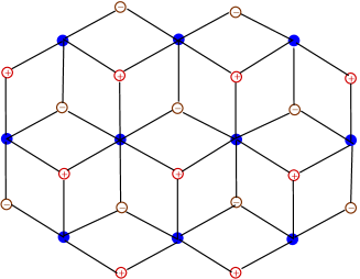
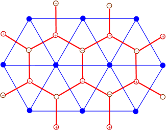
Figure 1. The diagonal staircase section as the bipartite quasiregular rhombic tiling (on the left), and the corresponding triangular and honeycomb lattices (on the right)

This is also the main idea behind the present paper. We derive the integrability properties of the self-adjoint linear problems on the triangular and honeycomb lattices from the corresponding properties of the three dimensional B-quadrilateral lattice. In particular, we obtain in this way the Darboux-type transformations for both linear problems, and we show that the Laplace transformations of [32] are nothing but a relation between two subsequent triangular sublattices of the B-quadrilateral lattice. We remark that the approach we use here is very close, in spirit, to the one used in [8, 5], where properties of the hexagonal circle patterns with constant intersection angles were derived from properties of an integrable system on the ${\mathbb{Z}}^{3}$ lattice, and to that used in [10], where discrete holomorphic functions on quad-graphs were constructed from discrete holomorphic functions on ${\mathbb{Z}}^{N}$. Our results can be also interpreted from the point of view of the discrete Cauchy–Riemann (discrete Moutard) equation on quad-graphs [9, 26], with the graph being the quasiregular rhombic tiling, as visualized on Figure 1. However, we would like to stress the multidimensional origin of our constructions and their geometric meaning.

The layout of the paper is as follows. In Section 2, after construction of the triangular and honeycomb grids as sublattices of the diagonal staircase section of the ${\mathbb{Z}}^{3}$ lattice (see Figure 1), we derive the self-adjoint 7-point scheme and the honeycomb linear problem from the discrete Moutard system. The sublattice approach provides the clear geometric meaning to the star-triangle relation between both linear problems. In Section 3 we present the corresponding interpretation of the Laplace transformation of the self-adjoint 7-point scheme [32] as the transition between subsequent triangular sublattices of the B-quadrilateral lattice. We introduce a 3D fully discrete novel integrable system describing such a transition. Finally, in Section 4 we obtain the Darboux transformations of the self-adjoint 7-point scheme [28] and the honeycomb linear problem from the Moutard transformation. In the rest of this introductory section we recall necessary informations on the discrete BKP equation, its linear problem (the discrete Moutard system), and the corresponding Moutard transformation.

1.3. The discrete Moutard system (the B-quadrilateral lattice)

Consider the system of discrete Moutard equations (the discrete BKP linear system) [11, 31]

(1.1) $$\psi_{ij}-\psi=f^{ij}\times(\psi_{i}-\psi_{j}),\qquad 1\leq i<j\leq N,$$

where $\psi:{\mathbb{Z}}^{N}\to{\mathbb{V}}$, and ${\mathbb{V}}$ is a linear space over a field $\mathbb{K}$, and $f^{ij}:{\mathbb{Z}}^{N}\to{\mathbb{K}}$, $1\leq i<j\leq N$, are some functions; here and in all the paper by a subscript we denote the shift in the corresponding discrete variable, i.e. $f_{i}(n_{1},\dots,n_{i},\dots,n_{N})=f(n_{1},\dots,n_{i}+1,\dots,n_{N})$.

Remark 1.1.

In [14] it was shown that the discrete Moutard system (1.1) characterizes algebraically (up to a gauge transformation) special quadrilateral lattices $x=[\psi]:{\mathbb{Z}}^{N}\to\mathbb{P}({\mathbb{V}})$ in the projectivization of ${\mathbb{V}}$, which satisfy the following additional local linear constraint: any point $x$ of the lattice and its neighbours $x_{ij}$, $x_{ik}$ and $x_{jk}$, for $i,j,k$ distinct, are coplanar.

The coefficients $f^{ij}$ are not arbitrary functions. Compatibility of the Moutard system leads to the following set of nonlinear equations [31]

(1.2) $$1+f^{jk}_{i}(f^{ij}-f^{ik})=f^{ik}_{j}f^{ij}=f^{ij}_{k}f^{ik},\qquad i,j,k\quad\text{distinct},$$

where, formally, we put $f^{ji}=-f^{ij}$.

If $\theta:{\mathbb{Z}}^{N}\to{\mathbb{K}}$ is a scalar solution of the system (1.1) then the solution $\tilde{\psi}:{\mathbb{Z}}^{N}\to{\mathbb{V}}$ of the Moutard transformation equations [31]

(1.3) $$\tilde{\psi}_{i}-\psi=\frac{\theta}{\theta_{i}}(\tilde{\psi}-\psi_{i}),\qquad 1\leq i\leq N,$$

satisfies a new discrete Moutard system with the fields

(1.4) $$\tilde{f}^{ij}=f^{ij}\frac{\theta_{i}\theta_{j}}{\theta_{ij}\theta}.$$

We will need also the fact that $\theta^{-1}$ satisfies the same Moutard system as the tranformed wave function $\tilde{\psi}$.

Remark 1.2.

The discrete Moutard transformation provides the algebraic part of the B-reduction of the fundamental transformation of the quadrilateral lattice [14]. This transformation acts within the class of B-quadrilateral lattices and, apart from the usual property of the fundamental transformation stating that the corresponding points $x$, $x_{i}$, $\tilde{x}$, $\tilde{x}_{i}$ of the two quadrilateral lattices are coplanar, we have the following additional linear constraint: the points $x$, $x_{ij}$, $\tilde{x}_{i}$ and $\tilde{x}_{j}$, for $i\neq j$, are coplanar as well.

2. Linear problems on the triangular and honeycomb lattices

The goal of this section is to present the derivation of the discrete Laplace equations on the triangular and honeycomb lattices from the system of Moutard equations on ${\mathbb{Z}}^{3}$. This is done in full detail to prepare the setting for the new results in Sections 3 and 4. The derivation of the Laplace equations from the discrete Moutard (Cauchy–Riemann) equations on planar bipartite quad-graphs is well known [26, 9]. The ${\mathbb{Z}}^{3}$ origin of some integrable systems on planar graphs was used in [8, 5], where properties of the hexagonal circle patterns with constant intersection angles were derived from properties of an integrable system on the ${\mathbb{Z}}^{3}$ lattice, and in [10], where discrete holomorphic functions on quad-graphs were constructed from discrete holomorphic functions on ${\mathbb{Z}}^{N}$.

2.1. The staircase section

Define the bipartition of the ${\mathbb{Z}}^{3}$ lattice depending if the sum of the coordinates is even (black points) or odd (white points). Consider the subset

$$V({\mathbb{T}})=\{m(1,1,0)+n(0,1,1):\;m,n\in{\mathbb{Z}}\}=\{(n_{1},n_{2},n_{2})\in{\mathbb{Z}}^{3}:\;n_{1}-n_{2}+n_{3}=0\},$$

of the black point lattice, which can be considered as the intersection of the ${\mathbb{Z}}^{3}$ lattice with the diagonal plane. Intersecting, instead, the ${\mathbb{Z}}^{3}$ lattice with two ”nearests” parallel planes we obtain the subsets

$$V({\mathbb{T}}_{+}) =\{(1,0,0)+m(1,1,0)+n(0,1,1):\;m,n\in{\mathbb{Z}}\}=\{(n_{1},n_{2},n_{2})\in{\mathbb{Z}}^{3}:\;n_{1}-n_{2}+n_{3}-1=0\},$$

$$V({\mathbb{T}}_{-}) =\{(0,1,0)+m(1,1,0)+n(0,1,1):\;m,n\in{\mathbb{Z}}\}=\{(n_{1},n_{2},n_{2})\in{\mathbb{Z}}^{3}:\;n_{1}-n_{2}+n_{3}+1=0\},$$

of the white point lattice. We call the union of the above sets, together with the corresponding edges and facets of the ${\mathbb{Z}}^{3}$ lattice, the diagonal staircase section of ${\mathbb{Z}}^{3}$ (see Figure 1). As a planar graph the diagonal staircase section is often refered to as quasiregular rhombic tiling (the dual of the kagome lattice).

Points of $V({\mathbb{T}})$ are vertices of the triangular grid ${\mathbb{T}}$ whose set of edges $E({\mathbb{T}})$ consists of segments connecting the nearest neighbours

$$E({\mathbb{T}})=\{[\boldsymbol{v}_{1},\boldsymbol{v}_{2}]:\;\boldsymbol{v}_{1},\boldsymbol{v}_{2}\in V({\mathbb{T}}),\;|\boldsymbol{v}_{1}-\boldsymbol{v}_{2}|=\sqrt{2}\}.$$

Similarly we define the triangular grids ${\mathbb{T}}_{\pm}$, which will be used in Section 3. However we will need first the honeycomb grid ${\mathbb{H}}$ whose set of vertices is $V({\mathbb{H}})=V({\mathbb{T}}_{+})\cup V({\mathbb{T}}_{-})$, and edges of which are the segments connecting points of $V({\mathbb{T}}_{\pm})$ with their nearest $V({\mathbb{T}}_{\mp})$ neighbours, see Figure 1

$$E({\mathbb{H}})=\{[\boldsymbol{v}_{+},\boldsymbol{v}_{-}]:\;\boldsymbol{v}_{+}\in V({\mathbb{T}}_{+}),\boldsymbol{v}_{-}\in V({\mathbb{T}}_{-}),\;|\boldsymbol{v}_{+}-\boldsymbol{v}_{-}|=\sqrt{2}\}.$$

We keep the bipartition of the honeycomb lattice into $\pm$-points. The honeycomb tiling is the dual of the triangular tiling (in the standard crystallographic sense). Roughly speaking, this means that the centers of the facets of one lattice are the vertices of the second one (see Figure 1).

2.2. The self-adjont 7 point scheme and the sublattice approach

The goal of this Section is to derive, using the sublattice approach, the self-adjoint 7-point scheme from the system of the Moutard equations on ${\mathbb{Z}}^{3}$ grid (the three dimensional B-quadrilateral lattice). However, we first recall a way (see, for example [10]) in which one can construct the Laplace equation for an arbitrary graph $\mathcal{G}$ with given weight functions $\nu:E(\mathcal{G})\to{\mathbb{K}}$ from non oriented edges to the field ${\mathbb{K}}$. When $\psi:V(\mathcal{G})\to{\mathbb{V}}$ is a function on vertices of the graph, then it satisfies the corresponding Laplace equation if at each vertex ${\boldsymbol{v}}_{0}$

(2.1) $$\sum_{{\boldsymbol{v}}\sim{\boldsymbol{v}}_{0}}\nu({\boldsymbol{v}},{\boldsymbol{v}}_{0})(\psi({\boldsymbol{v}})-\psi({\boldsymbol{v}}_{0}))=0,$$

where the summation is over vertices adjacent to ${\boldsymbol{v}}_{0}$.

In the case of the triangular grid there are three families of edges, and therefore function $\nu$ gives rise to three functions, say $a,b$ and $s$, given on triangular lattice; see Figure 2, where also the corresponding convention of labeling directions $I$ and $I\!I$ of the lattice is given.

Figure 2. The triangular lattice, its main directions and the fields $a,b,s$ on its edges

The Laplace equation on such weighted graph reads

(2.2) $$a(\psi_{I}-\psi)+a_{-I}(\psi_{-I}-\psi)+b(\psi_{II}-\psi)+b_{-I\!I}(\psi_{-I\!I}-\psi)+s_{I}(\psi_{I,-I\!I}-\psi)+s_{II}(\psi_{-I,I\!I}-\psi)=0,$$

where $\psi:V({\mathbb{T}})\to{\mathbb{V}}$ is a field defined in the vertices of the grid with values in a vector space ${\mathbb{V}}$. It is easy to see that given any solution $\psi:{\mathbb{Z}}^{3}\to{\mathbb{V}}$ of the the Moutard linear system (1.1), then its restriction to the vertices $V({\mathbb{T}})$ of the triangular lattice satisfies the self-adjoint affine 7-point scheme (2.2) with the edge fields defined as

(2.3) $$a=\frac{1}{f^{12}},\qquad b=\frac{1}{f^{23}},\qquad s=-f^{13}_{-1-2-3},$$

and the shifts on the triangular lattice given by

(2.4) $$(I)=(12),\qquad\text{and}\qquad(II)=(23).$$

Equation (2.2) is the affine form of the general self-adjoint scheme on the triangular grid

(2.5) $$A\Psi_{I}+A_{-I}\Psi_{-I}+B\Psi_{II}+B_{-I\!I}\Psi_{-I\!I}+S_{I}\Psi_{I,-I\!I}+S_{II}\Psi_{-I,I\!I}=F\Psi,$$

considered in [32]. In this paper we confine ourselves to consideration of the affine scheme (2.2) (without loss of generality because, as we will see below, every scheme (2.5) can be transformed to an affine form (2.2) by means of gauge transformation).

Corollary 2.1.

Given a scalar solution $\sigma$ of the generic self-adjoint 7-point scheme (2.5), then $\psi=\Psi/\sigma$ satisfies the affine self-adjoint 7-point scheme (2.2) with the coefficients

(2.6) $$a=A\sigma_{I}\sigma,\qquad b=B\sigma_{I\!I}\sigma,\qquad s=S\sigma_{-I}\sigma_{-I\!I}.$$

Conversely, given a generic function $\rho:V({\mathbb{T}})\to{\mathbb{K}}$ on the triangular grid and given a solution $\psi:V({\mathbb{T}})\to{\mathbb{V}}$ of the self-adjoint 7-point scheme (2.2), then the function $\Psi=\psi/\rho$ satisfies the scheme (2.5) with the coefficients

(2.7) $$A=a\rho_{I}\rho,\qquad B=b\rho_{I\!I}\rho,\qquad S=s\rho_{-I}\rho_{-I\!I},\qquad F=(a+a_{-I}+b+b_{-I\!I}+s_{I,-I\!I}+s_{-I,I\!I})\rho^{2}.$$

Remark 2.2.

Since the Moutard equation on the ${\mathbb{Z}}^{N}$ grid can be integrated by the finite gap method [21], the above sublattice derivation of the 7-point scheme from the discrete Moutard equations imply that also the 7-point scheme on the triangular lattice can be integrated using the theory developed in [21, 14].

Remark 2.3.

Notice that the above derivation of the self-adjoint affine 7-point scheme can be generalized to arbitrary dimension as follows. Consider a solution $\psi:{\mathbb{Z}}^{N}\to{\mathbb{V}}$ of the the $N$-dimensional Moutard linear system (1.1) on the $2N$ elementary quadrilaterals

$$(1,2),\dots,(j,j+1),\dots,(N-1,N),(N,-1),(-1,-2),\dots,(-N,1).$$

Add the first $N$ schemes and substract the remaining ones (dividing by the Moutard coefficients, when necessary). The result is the following self-adjoint $(2N+1)$-point scheme (on a star with $2N$ legs) on the black points:

(2.8) $$\sum_{j=1}^{N-1}\left(\frac{\psi_{j,j+1}-\psi}{f^{j,j+1}}+\frac{\psi_{-j,-j-1}-\psi}{f^{j,j+1}_{-j,-j-1}}\right)=f^{1,N}_{-1}(\psi_{-1,N}-\psi)+f^{1,N}_{-N}(\psi_{1,-N}-\psi).$$

2.3. The linear problem on the honeycomb lattice

The discrete Moutard equations (1.1) imply a linear relation between a point of the ${\mathbb{T}}_{-}$ lattice with its three nearest ${\mathbb{T}}_{+}$ neighbours:

(2.9) $$f^{12}(\psi_{1}-\psi_{2})+f^{23}(\psi_{3}-\psi_{2})-\frac{1}{f^{13}_{2}}(\psi_{123}-\psi_{2})=0,$$

and a linear relation between a point of the ${\mathbb{T}}_{+}$ lattice with its three nearest ${\mathbb{T}}_{-}$ neighbours:

(2.10) $$f^{12}(\psi_{2}-\psi_{1})+f^{23}_{1-3}(\psi_{12-3}-\psi_{1})-\frac{1}{f^{13}_{-3}}(\psi_{-3}-\psi_{1})=0.$$

These two relations, which give the geometric characterization of the B-quadrilateral lattice [14], can be interpreted as the following linear self-adjoint system of equations on the honeycomb white lattice (see Figure 3)

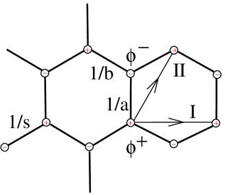
Figure 3. The honeycomb lattice

(2.11) $$\frac{1}{a}(\phi^{+}-\phi^{-})+\frac{1}{b}(\phi^{+}_{-I,I\!I}-\phi^{-})+\frac{1}{s_{I,I\!I}}(\phi^{+}_{I\!I}-\phi^{-}) =0,$$

(2.12) $$\frac{1}{a}(\phi^{-}-\phi^{+})+\frac{1}{b_{I,-I\!I}}(\phi^{-}_{I,-I\!I}-\phi^{+})+\frac{1}{s_{I}}(\phi^{-}_{-I\!I}-\phi^{+}) =0.$$

for the fields $\phi^{+}$ and $\phi^{-}$, defined by

(2.13) $$\phi^{+}=\psi_{1},\qquad\phi^{-}=\psi_{2},$$

having used also (2.3) and the triangular lattice shifts (2.4).

Again, like in the triangular lattice, one can consider a more general linear system on the honeycomb lattice than the above affine one (2.11)-(2.12). The result below is the analogue of Corollary 2.1 for the honeycomb lattice.

Corollary 2.4.

Given a solution $(\sigma^{+},\sigma^{-})$ of the generic honeycomb system

(2.14) $$\frac{1}{A}\Phi^{+}+\frac{1}{B}\Phi^{+}_{-I,I\!I}+\frac{1}{S}_{I,II}\Phi^{+}_{I\!I} =F^{+}\Phi^{-},$$

(2.15) $$\frac{1}{A}\Phi^{-}+\frac{1}{B_{I,-I\!I}}\Phi^{-}_{I,-I\!I}+\frac{1}{S}_{I}\Phi^{-}_{-I\!I} =F^{-}\Phi^{+},$$

then $(\phi^{+},\phi^{-})$, where $\phi^{\pm}=\Phi^{\pm}/\sigma^{\pm}$, satisfies the affine honeycomb linear system (2.11)-(2.12) with the coefficients

(2.16) $$a=\frac{A}{\sigma^{+}\sigma^{-}},\qquad b=\frac{B}{\sigma^{+}_{-I,I\!I}\sigma^{-}},\qquad s=\frac{S}{\sigma^{+}_{-I}\sigma^{-}_{-I,-I\!I}}.$$

Conversely, given generic function $(\rho^{+},\rho^{-}):V({\mathbb{H}})\to{\mathbb{K}}$ on the honeycomb grid, and given a solution $(\phi^{+},\phi^{-}):V({\mathbb{H}})\to{\mathbb{V}}$ of the linear problem (2.11)-(2.12), then the function $(\Phi^{+},\Phi^{-})=(\phi^{+}/\rho^{+},\phi^{-}/\rho^{-})$ satisfies the system (2.14)-(2.15) (2.5) with the coefficients

$$A=\frac{a}{\rho^{+}\rho^{-}},\qquad B=\frac{b}{\rho^{+}_{-I,I\!I}\rho^{-}},\qquad S=\frac{s}{\rho^{+}_{-I}\rho^{-}_{-I,-I\!I}},$$

$$F^{+}=(\rho^{-})^{2}\left(\frac{1}{a}+\frac{1}{b}+\frac{1}{s_{I,I\!I}}\right),\qquad F^{-}=(\rho^{+})^{2}\left(\frac{1}{a}+\frac{1}{b_{I,-I\!I}}+\frac{1}{s_{I}}\right).$$

2.4. The duality between the linear problems on the triangular and the honeycomb lattices

As we have already remarked, the honeycomb and triangular tilings are dual to each other. In fact, the duality can be extended to the level of the linear problems. Both the honeycomb linear system (2.11)-(2.12) and the self-adjoint affine 7-point system (2.2) are consequences of the following ”duality” equations between function $\psi$ on the ${\mathbb{T}}$ lattice and the pair $(\phi^{+},\phi^{-})$ on the honeycomb lattice

(2.17) $$\psi_{I}-\psi =\frac{1}{a}(\phi^{+}-\phi^{-}),$$

(2.18) $$\psi_{I\!I}-\psi =\frac{1}{b}(\phi^{-}-\phi^{+}_{-I,I\!I}),$$

(2.19) $$\psi_{I\!I}-\psi_{I} =\frac{1}{s_{I,I\!I}}(\phi^{+}_{I\!I}-\phi^{-}).$$

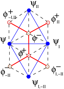
Figure 4. The star-triangle duality relations between the triangular and the honeycomb tilings; the dashed lines represent the edges of the quasiregular rhombic tiling (the staircase diagonal section)

Notice that the star-triangle equations (2.17)-(2.19) are just the Moutard equations on the diagonal staircase section. Equations (2.17)-(2.19) have a point of ${\mathbb{T}}_{-}$ as the star center, while equations (2.17), (2.18)${}_{I,-I\!I}$ and (2.19)${}_{-I\!I}$ have a point of ${\mathbb{T}}_{+}$ as the star center (see Figure 4). This is the direct counterpart of the famous star-triangle relation widely used in the analysis of solvable models in statistical mechanics [6]. As it was shown in [24] the (nonlinear) star-triangle transformation in electric networks, interpreted as the local Yang-Baxter equation, leads to Miwa’s discrete BKP equation. The (linear) star-triangle relation (2.17)-(2.19) gives thus the linear problem for the nonlinear one (see also Remark 3.3).

Remark 2.5.

The above star-triangle relation can be considerd as a particular case of the relation between the Laplace equations obtained from the discrete Cauchy–Riemann (discrete Moutard) equation on quad-graphs [9], where the graph is the quasiregular rhombic tiling. However, we would like to stress the three dimensional (not planar) origin of our construction and its geometric meaning.

3. The Laplace transformation of the triangular lattice

The Laplace transformations of the self-adjoint 7-point scheme on the triangular lattice were defined in [32] and studied in [34, 22]. The construction used in [32] consists in the factorization (up to a multiplication operator summand) of the second order operator (2.5) into product of two first order operators. In this Section we will present the geometric meaning of the Laplace transformations. The basic idea is as follows: the hyperplanes

$${\mathbb{T}}_{\ell}=\{(n_{1},n_{2},n_{2})\in{\mathbb{Z}}^{3},\;n_{1}-n_{2}+n_{3}=\ell\},\qquad\ell\in{\mathbb{Z}},$$

foliate the bipartite ${\mathbb{Z}}^{3}$ lattice into triangle lattices of a fixed (black for $\ell$ even, and white for $\ell$ odd) colour. The transition between two subsequent lattices of the same colour is the Laplace transformation.

To develop algebraically this idea we will use formulas (2.11)-(2.12) of the affine honeycomb linear system, which can be considered as the connection formulas between the affine self-adjoint 7-point schemes on ${\mathbb{T}}_{\pm 1}={\mathbb{T}}_{\pm}$ lattices. To simplify our calculations we will work in the affine gauge induced by the Moutard linear problems (in [32, 34] generic gauge was used). Notice that, in the (forward) transition from ${\mathbb{T}}_{-}$ to ${\mathbb{T}}_{+}$, we have three natural possibilities (see Figure 4)

$$\phi^{-}\to\phi^{+},\quad\phi^{-}\to\phi^{+}_{I\!I},\quad\phi^{-}\to\phi^{+}_{-I,I\!I}.$$

This ambiguity and the corresponding one for the backward transition was observed on the algebraic level in [34]. In this article we choose the transition $\phi^{-}\to\phi^{+}$ (the others can be obtained by simple shifts) as the forward Laplace transformation $\mathcal{L}^{+}$.

The second equation (2.12) of the honeycomb linear problem can be rewritten in the form

(3.1) $$\phi^{+}=\mathcal{L}^{+}\phi^{-}=\frac{1}{r_{I}}\left(b_{I,-I\!I}s_{I}\phi^{-}+ab_{I,-I\!I}\phi^{-}_{-I\!I}+as_{I}\phi^{-}_{I,-I\!I}\right),$$

where

(3.2) $$r=a_{-I}s+b_{-I\!I}s+a_{-I}b_{-I\!I}.$$

Remark 3.1.

The above transformation is the affine version of the Laplace transformation $P_{2}$ of [34].

Inserting such $\phi^{+}$ into the second equation of the linear system (2.11)-(2.12), we obtain that the field $\phi^{-}$ satisfies the affine self-adjoint 7-point scheme with the coefficients

(3.3) $$a^{-}=-\frac{a_{I\!I}}{r_{I,I\!I}},\qquad b^{-}=-\frac{b_{I}}{r_{I,I\!I}},\qquad s^{-}=-\frac{s}{r}.$$

Remark 3.2.

The coefficients are given up to a common constant multiplier. The above choice is motivated by the sublattice approach. Indeed, equations (2.13) and (2.3) imply that, in the sublattice notation

$$a^{-}=\frac{1}{f^{12}_{2}},\qquad b^{-}=\frac{1}{f^{23}_{2}},\qquad s^{-}=-f^{13}_{-1-3}.$$

We leave it for the Reader to check that equations (3.3) are consequences of the discrete BKP equations (1.2).

Remark 3.3.

Equations (3.3) are directly related to the star-triangle transformations in electrical (or spring) networks, see for example [24], between the conductivities of conductors (stiffness of the springs); compare also Section 2.4.

The above equation can be reversed, i.e., the coefficients $a,b,s$ can be expressed in terms of $a^{-},b^{-},s^{-}$ as

(3.4) $$a=-\frac{a^{-}_{-I\!I}}{q^{-}_{-I\!I}},\qquad b=-\frac{b^{-}_{-I}}{q^{-}_{-I}},\qquad s=-\frac{s^{-}}{q^{-}_{-I,-I\!I}},\qquad\text{where}\qquad q^{-}=a^{-}b^{-}+a^{-}s^{-}_{I,I\!I}+b^{-}s^{-}_{I,I\!I}=\frac{1}{r_{I,I\!I}}.$$

This allows to write down the forward Laplace transform of $\phi^{-}$ in terms of coefficients (3.3) of the scheme on ${\mathbb{T}}_{-}$

(3.5) $$\phi^{+}=\mathcal{L}^{+}\phi^{-}=\frac{1}{q^{-}_{-I\!I}}\left(b^{-}_{-I\!I}s^{-}_{I}\phi^{-}+a^{-}_{-I}b^{-}_{-I\!I}\phi^{-}_{-I\!I}+a^{-}_{-I}s^{-}_{I}\phi^{-}_{I,-I\!I}\right).$$

Similarly, the backward transformation of $\phi^{+}$

(3.6) $$\phi^{-}=\mathcal{L}^{-}\phi^{+}=\frac{1}{q}\left(bs_{I,I\!I}\phi^{+}+ab\phi^{+}_{I\!I}+as_{I,I\!I}\phi^{+}_{-I,I\!I}\right),$$

where

(3.7) $$q=as_{I,I\!I}+bs_{I,I\!I}+ab,$$

inserted into the first equation of the linear problem gives the affine self-adjoint 7-point scheme with the coefficients

(3.8) $$a^{+}=-\frac{a_{I,-I\!I}}{q_{I,-I\!I}},\qquad b^{+}=-\frac{b}{q},\qquad s^{+}=-\frac{s_{I}}{q_{-I\!I}}.$$

Remark 3.4.

Again, the above coefficients can be obtained by the sublattice approach, i.e.,

$$a^{+}=\frac{1}{f^{12}_{1}},\qquad b^{+}=\frac{1}{f^{23}_{1}},\qquad s^{+}=-f^{13}_{-2-3},$$

and equations (3.8) are consequences of the nonlinear discrete BKP equations (1.2).

The inversion formulas

(3.9) $$a=-\frac{a^{+}_{-I,I\!I}}{r^{+}_{I\!I}},\qquad b=-\frac{b^{+}}{r^{+}_{I\!I}},\qquad s=-\frac{s^{+}_{-I}}{r^{+}_{-I}},\qquad\text{where}\qquad r^{+}=a^{+}_{-I}b^{+}_{-I\!I}+a^{+}_{-I}s^{+}+b^{+}_{-I\!I}s^{+}=\frac{1}{q_{-I\!I}},$$

allow to write down the backward Laplace transform of $\phi^{+}$ in terms of coefficients (3.8) of the scheme on ${\mathbb{T}}_{+}$

(3.10) $$\phi^{-}=\mathcal{L}^{-}\phi^{+}=\frac{1}{r^{+}_{I\!I}}\left(b^{+}s^{+}_{I,I\!I}\phi^{+}+a^{+}_{-I,I\!I}b^{+}\phi^{+}_{I\!I}+a^{+}_{-I,I\!I}s^{+}_{I,I\!I}\phi^{+}_{-I,I\!I}\right).$$

We have obtained therefore the sublattice derivation of the Laplace transform, which we formulate in terms of the proposition below.

Proposition 3.5.

Given a solution $\phi^{-}$ of the self-adjoint affine 7-point scheme with coefficients (3.3), then its Laplace transform $\phi^{+}=\mathcal{L}^{+}\phi^{-}$, given by formula (3.5), satisfies a new self-adjoint affine 7-point scheme on ${\mathbb{T}}_{+}$ whose coefficients can be obtained from those of ${\mathbb{T}}^{-}$ by inserting expressions (3.4) for functions $a,b,s$ into equations (3.8). The inverse Laplace transform from $\phi^{+}$ to $\phi^{-}=\mathcal{L}^{-}\phi^{+}$ is given by equation (3.10).

Corollary 3.6.

Interpreting the Laplace transformation as a shift in a new discrete variable $K\in{\mathbb{Z}}$, from equations (3.4) and (3.9) one can write down a nonlinear system relating coefficients of the subsequent 7-point equations

(3.11) $$\frac{a^{K}_{-I\!I}}{q^{K}_{-I\!I}}=\frac{a^{K+1}_{-I,I\!I}}{r^{K+1}_{I\!I}},\qquad\frac{b^{K}_{-I}}{q^{K}_{-I}}=\frac{b^{K+1}}{r^{K+1}_{I\!I}},\qquad\frac{s^{K}}{q^{K}_{-I,-I\!I}}=\frac{s^{K+1}_{-I}}{r^{K+1}_{-I}},$$

where

(3.12) $$q^{K}=a^{K}b^{K}+a^{K}s^{K}_{I,I\!I}+b^{K}s^{K}_{I,I\!I},\qquad r^{K}=a^{K}_{-I}b^{K}_{-I\!I}+a^{K}_{-I}s^{K}+b^{K}_{-I\!I}s^{K}.$$

Remark 3.7.

As we have seen, the discrete (3D) BKP equations (1.2) can be interpreted as the connection formulas (or the discrete time evolution) between subsequent self-adjoint problems on the triangular lattices $\mathbb{T}_{\ell}$, $\ell\in\mathbb{Z}$. This implies also that one can obtain the full Mutard system on the ${\mathbb{Z}}^{3}$ lattice from the self-adjoint linear problem on the triangular lattice (or the honeycomb lattice).

Remark 3.8.

The novel, up to our knowledge, nonlinear system (3.11)-(3.12) is the sublattice version of the discrete BKP equations. It describes the transformation rule of the coefficients of self-adjoint 7-point schemes under the Laplace transformation. The corresponding transformation rule in the case of the discrete affine hyperbolic 4-point scheme is equivalent to Hirota’s discrete Toda system [23], and was derived in [12] (see also [13]). Its geometric counterpart is given by the Laplace transforms of two dimensional discrete conjugate nets, introduced in pure geometric way by Sauer [36]. The Laplace transform of the hyperbolic 4-point operator (in general gauge) was also defined independently, using the factorization technique, in [32].

We would like to close this Section by presenting the decomposition of the affine self-adjoint 7-point scheme in the spirit of the papers [32, 22] (formulas below are the affine versions of the corresponding formulas in there). Denote by $T_{I}$ and $T_{I\!I}$ the standard translation operators along directions $I$ and $I\!I$ of the triangular lattice. Combining both Laplace transform (3.1) and (3.6) we obtain equations

$$\phi^{+} =\left[\frac{1}{r_{I}}\left(b_{I,-I\!I}s_{I}+ab_{I,-I\!I}T_{I\!I}^{-1}+as_{I}T_{I}T_{I\!I}^{-1}\right)\right]\left[\frac{1}{q}\left(bs_{I,I\!I}+abT_{I\!I}+as_{I,I\!I}T_{I}T_{I\!I}^{-1}\right)\right]\phi^{+},$$

$$\phi^{-} =\left[\frac{1}{q}\left(bs_{I,I\!I}+abT_{I\!I}+as_{I,I\!I}T_{I}T_{I\!I}^{-1}\right)\right]\left[\frac{1}{r_{I}}\left(b_{I,-I\!I}s_{I}+ab_{I,-I\!I}T_{I\!I}^{-1}+as_{I}T_{I}T_{I\!I}^{-1}\right)\right]\phi^{-},$$

i.e., ”factorized” linear problems on ${\mathbb{T}}_{+}$ and ${\mathbb{T}}_{-}$. Notice that the fields $a$, $b$, $s$ are the coefficients of the self-adjoint 7-point scheme (2.2) of the intermediate black-point lattice ${\mathbb{T}}_{0}$.

Elaborating the above formulas, one can derive the following decomposition of the affine Laplace operator of the lattice $\phi^{-}$ (we leave the case of $\phi^{+}$ to the Reader)

(3.13) $$\left[Q^{-}(Q^{-})^{*}-w^{-}\right]\phi^{-}=0,$$

in terms of the operator

$$Q^{-}=x^{-}+y^{-}T_{I\!I}+z^{-}T_{I}^{-1}T_{I\!I},$$

and its formal adjoint

$$(Q^{-})^{*}=x^{-}+T_{I\!I}^{-1}y^{-}+T_{I}T_{I\!I}^{-1}z^{-},$$

where

$$(x^{-})^{2}=\frac{b^{-}_{-I\!I}s^{-}_{I}}{a^{-}_{-I\!I}},\qquad(y^{-})^{2}=\frac{a^{-}b^{-}}{s^{-}_{I,I\!I}},\qquad(z^{-})^{2}=\frac{a^{-}_{-I}s^{-}_{I\!I}}{b^{-}_{-I}},$$

$$w^{-}=\frac{q^{-}_{-I\!I}}{a^{-}_{-I\!I}}+\frac{q^{-}_{-I}}{b^{-}_{-I}}+\frac{q^{-}}{s^{-}_{I,I\!I}}.$$

Remark 3.9.

In [34] the relation between the coefficients (3.3) of the 7-point scheme on ${\mathbb{T}}_{-}$ and the corresponding coefficients of $Q^{-}$ has been brought to the form

$$a^{-}=y^{-}z^{-}_{I},\qquad b^{-}=y^{-}x^{-}_{I\!I},\qquad s^{-}=x^{-}_{-I}z^{-}_{-I\!I},$$

$$w^{-}=(x^{-})^{2}+(y^{-})^{2}+(z^{-})^{2}+a^{-}+a^{-}_{-I}+b^{-}+b^{-}_{-I\!I}+s^{-}_{I}+s^{-}_{I\!I}.$$

Remark 3.10.

In the special case $x=y=z=1$ the operator $Q$ and its adjoint $Q^{*}$ were viewed in [22] as the analogs of the operators $\partial$ and $\bar{\partial}$ in the discrete holomorphic function theory. In [25] the Dirac operator on more general bipartite planar graphs was defined and related to the dimer model of statistical mechanics.

Remark 3.11.

The Laplace transformation equations (3.1) and (3.6) are nothing but the linear problem (2.11)-(2.12) on the honeycomb lattice. Conversely, the factorization (3.13) implies the honeycomb linear problem.

4. The Darboux transformations

Our goal here is to derive the Darboux transformation of the self-adjoint 7-point scheme [28] and of the linear honeycomb problem using the sublattice approach. In doing that we will follow the corresponding ideas of [21], where the Darboux transformation of the self-adjoint 5-point scheme [28] was rederived in such a way.

4.1. The Darboux transformation of the linear problem on the triangular lattice

Before presenting the sublattice derivation of the Darboux transformation, let us first comment on the geometric content of the calculations below. The geometric definition [14] of the B-quadrilateral lattice states that there exists a linear relation between $\psi$, $\psi_{-1-2}$, $\psi_{-1-3}$ and $\psi_{-2-3}$; i.e., the corresponding points $[\psi]$, $[\psi_{-1-2}]$, $[\psi_{-1-3}]$, $[\psi_{-2-3}]$ of the projectivization of ${\mathbb{V}}$ are coplanar. Similarly, the geometric definition of the corresponding reduction of the fundamental transformation states that there exists a linear relation between $\psi_{-1-3}$, $\psi_{-2-3}$, $\tilde{\psi}_{-3}$ and $\tilde{\psi}_{-1-2-3}$. Both corresponding planes intersect along the line passing through $[\psi_{-1-2}]$ and $[\psi_{-1-3}]$, which means that all the six points belong to a three dimensional subspace. Therefore any five of the six points are linearly related (see Figure 5). This allows, in particular, for the elimination of $\psi_{-1-3}$, which does not belong to the allowed subset $V({\mathbb{T}})$ of the ${\mathbb{Z}}^{3}$ lattice, yelding a linear relation between $\psi$, $\psi_{-1-2}$, $\psi_{-2-3}$, $\tilde{\psi}_{-3}$ and $\tilde{\psi}_{-1-2-3}$, the first equation of the Darboux transformation.

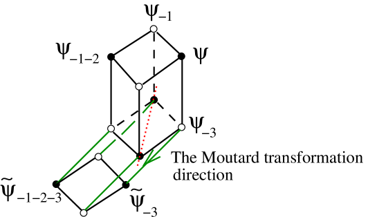
Figure 5. Geometry of the sublattice approach to the Darboux transformation of the self-adjoint 7-point scheme

Three discrete Moutard equations (1.1), shifted in $(-i-j)$ directions, lead to the linear equation

(4.1) $$\frac{1}{f^{12}_{-1-2}}(\psi-\psi_{-1-2})-\frac{1}{f^{13}_{-1-3}}(\psi-\psi_{-1-3})+\frac{1}{f^{23}_{-2-3}}(\psi-\psi_{-2-3})=0.$$

If $\theta$ is a scalar solution of the system (1.1), then the Moutard transformations (1.3) for $i=1,2$, taken with appropriate shifts, and the discrete Moutard equation, shifted in the $(-1-2-3))$ direction, give

(4.2) $$\frac{\theta_{-3}}{\theta_{-2-3}}(\tilde{\psi}_{-3}-\psi_{-2-3})-\frac{\theta_{-3}}{\theta_{-1-3}}(\tilde{\psi}_{-3}-\psi_{-1-3})-\frac{1}{\tilde{f}^{12}_{-1-2-3}}(\tilde{\psi}_{-3}-\tilde{\psi}_{-1-2-3})=0.$$

The elimination of $\psi_{-1-3}$ from equations (4.1) and (4.2) leads to

(4.3) $$\tilde{\psi}_{-3}+\frac{\theta_{-1-3}}{\theta_{-3}}\frac{1}{\tilde{f}^{12}_{-1-2-3}}(\tilde{\psi}_{-3}-\tilde{\psi}_{-1-2-3})-\frac{\theta_{-1-3}}{\theta_{-2-3}}(\tilde{\psi}_{-3}-\psi_{-2-3})=\\ \psi-\frac{f^{13}_{-1-3}}{f^{12}_{-1-2}}(\psi-\psi_{-1-2})-\frac{f^{13}_{-1-3}}{f^{23}_{-2-3}}(\psi-\psi_{-2-3}).$$

We multiply both sides by $f^{13}_{-1-2-3}\theta_{-2-3}f^{12}_{-1-2}/f^{13}_{-1-3}$, and we use (a part of) the nonlinear equations (1.2):

(4.4) $$f^{13}_{-1-3}f^{12}_{-1-2-3}=f^{12}_{-1-2}f^{13}_{-1-2-3},$$

(4.5) $$\frac{1}{f^{13}_{-1-2-3}}=f^{23}_{-2-3}+f^{12}_{-1-2}-\frac{f^{23}_{-2-3}f^{12}_{-1-2}}{f^{13}_{-1-3}},$$

to transform equation (4.3) into

(4.6) $$\theta_{-3}\tilde{\psi}_{-3}-\theta_{-1-2-3}\tilde{\psi}_{-1-2-3}=-\frac{\theta_{-2-3}}{f^{23}_{-2-3}}\psi+f^{13}_{-1-2-3}\theta_{-2-3}\psi_{-1-2}+\left(\frac{\theta}{f^{23}_{-2-3}}-f^{13}_{-1-2-3}\theta_{-1-2}\right)\psi_{-2-3}.$$

Similar considerations, with equation

(4.7) $$\frac{\theta_{-1}}{\theta_{-1-3}}(\tilde{\psi}_{-1}-\psi_{-1-3})-\frac{\theta_{-1}}{\theta_{-1-2}}(\tilde{\psi}_{-1}-\psi_{-1-2})-\frac{1}{\tilde{f}^{23}_{-1-2-3}}(\tilde{\psi}_{-1}-\tilde{\psi}_{-1-2-3})=0$$

instead of equation (4.2), lead to

(4.8) $$\theta_{-1}\tilde{\psi}_{-1}-\theta_{-1-2-3}\tilde{\psi}_{-1-2-3}=\frac{\theta_{-1-2}}{f^{12}_{-1-2}}\psi-f^{13}_{-1-2-3}\theta_{-1-2}\psi_{-2-3}-\left(\frac{\theta}{f^{12}_{-1-2}}-f^{13}_{-1-2-3}\theta_{-2-3}\right)\psi_{-1-2}.$$

Introducing the field $\hat{\psi}=\theta_{-1-2-3}\tilde{\psi}_{-1-2-3}$ and using the sublattice notation (2.3), the above system (4.6) and (4.8) is rewritten in the form

(4.9) $$\hat{\psi}_{I}-\hat{\psi}\; =-b_{-I\!I}\theta_{-I\!I}\psi-s\theta_{-I\!I}\psi_{-I}+(b_{-I\!I}\theta+s\theta_{-I})\psi_{-I\!I},$$

(4.10) $$\hat{\psi}_{I\!I}-\hat{\psi} =\;\;\;a_{-I}\theta_{-I}\psi+s\theta_{-I}\psi_{-II\!}-(a_{-I}\theta+s\theta_{-I\!I})\psi_{-I}.$$

Because $\tilde{\psi}$ and $\theta^{-1}$ satisfy the same Moutard system, then they satisfy the same self-adjoint affine 7-point scheme. By Corollary 2.1, the function $\hat{\psi}$ satisfies the self-adjoint affine 7-point scheme whose coefficients can be found from equations (2.3), with $\tilde{f}^{ij}$ in place of $f^{ij}$, supplemented by the $(-1-2-3)$ shift and by the change (2.6), with respect to the above-mentioned gauge, with $\sigma=1/\theta_{-1-2-3}$. This implies that the coefficients read

$$\hat{a} =\frac{1}{\tilde{f}^{12}_{-1-2-3}\theta_{-3}\theta_{-1-2-3}}=\frac{1}{f^{12}_{-1-2-3}\theta_{-2-3}\theta_{-1-3}},$$

$$\hat{b} =\frac{1}{\tilde{f}^{23}_{-1-2-3}\theta_{-1}\theta_{-1-2-3}}=\frac{1}{f^{23}_{-1-2-3}\theta_{-1-2}\theta_{-1-3}},$$

$$\hat{s}_{II\!I} =-\tilde{f}^{13}_{-1-3}\frac{1}{\theta_{-1}\theta_{-3}}=-f^{13}_{-1-3}\frac{1}{\theta\theta_{-1-3}}.$$

To rewrite them in the sublattice notation we notice that equation (4.5) can be rewritten in the form

(4.11) $$\frac{1}{f^{13}_{-1-3}}=\frac{r}{s},\qquad$$

where $r$ is given by (3.2). Then equation (4.4) and its analogue for $f^{23}$ give

(4.12) $$\frac{1}{f^{12}_{-1-2-3}}=-\frac{a_{-I}}{r},\qquad\frac{1}{f^{23}_{-1-2-3}}=-\frac{b_{-I\!I}}{r}.$$

Finally, equation (4.1), satisfied by $\theta$, and equation (4.11) imply

(4.13) $$\frac{\theta_{-1-3}}{f^{13}_{-1-3}}=a_{-I}\theta_{-I}+b_{-I\!I}\theta_{-I\!I}+\frac{\theta a_{-I}b_{-I\!I}}{s},$$

which gives

(4.14) $$\hat{a}=-\frac{a_{-I}}{\theta_{-I\!I}p},\qquad\hat{b}=-\frac{b_{-I\!I}}{\theta_{-I}p},\qquad\hat{s}_{II\!I}=-\frac{s}{\theta p},$$

where

(4.15) $$p=s(a_{-I}\theta_{-I}+b_{-I\!I}\theta_{-I\!I})+a_{-I}b_{-I\!I}\theta.$$

Finally we can formulate the theorem, which was given (in the equivalent non-affine form, see Remark 4.2 below) in [28] directly on the 7-point level.

Theorem 4.1.

Given the general solution $\psi$ of the affine self-adjoint 7-point scheme (2.2), and given its particular solution $\theta$, then equations (4.9) and (4.10) define the general solution $\hat{\psi}$ of the affine self-adjoint 7-point scheme with coefficients given by formulas (4.14)-(4.15).

Remark 4.2.

Equations (4.9) and (4.10) and the transformation formulas (4.14) for the coefficients coincide with equations (32) and (34) in [28]. The identification $\hat{\psi}=\psi^{\prime}\theta$, where $\psi^{\prime}$ is the corresponding transform in [28], implies that $\psi^{\prime}$ satisfies a self-adjoint 7-point scheme (an arbitrary gauge does not change the structure of the equation) which will not have, in general, the affine form.

Remark 4.3.

One could consider another (equivalent) choice of the Darboux transformation direction, for example $\psi\to\theta_{123}\tilde{\psi}_{123}$. This would change slightly the Darboux transformation equations (4.9) and (4.10) and formulas (4.14)-(4.15).

Remark 4.4.

Notice that, for $\psi$ defined on $V({\mathbb{T}})$, the sum of the $n_{1}$, $n_{2}$ and $n_{3}$ coordinates of $\tilde{\psi}_{-1-2-3}$ is odd. However, it is convenient not to considered $\tilde{\psi}_{-1-2-3}$ as a field defined in points of the white lattice. The proper interpretation would be to consider the Moutard transformation direction as a shift in the fourth dimension of the ${\mathbb{Z}}^{4}$ lattice. Then the sum of all coordinates (including $n_{4}=1$) of $\tilde{\psi}_{-1-2-3}$ is even.

4.2. The Darboux transformation of the integrable honeycomb lattice

In this last part of the paper we first state the theorem on the Darboux transformation of the honeycomb linear problem, and then we show its sublattice derivation.

Theorem 4.5.

Given the general solution $(\phi^{+},\phi^{-})$ of the honeycomb linear system (2.11)-(2.12), and given its particular solution $(\theta^{+},\theta^{-})$, then the solution $(\check{\phi}^{+},\check{\phi}^{-})$ of the system

(4.16) $$\check{\phi}^{+}_{I\!I}-\check{\phi}^{-} =\frac{s}{r}\left(\theta^{-}_{-I\!I}\phi^{-}_{-I}-\theta^{-}_{-I}\phi^{-}_{-I\!I}\right),$$

(4.17) $$\check{\phi}^{+}-\check{\phi}^{-} =\frac{a_{-I}}{r}\left(\theta^{-}_{-I,-I\!I}\phi^{-}_{-I\!I}-\theta^{-}_{-I\!I}\phi^{-}_{-I,-I\!I}\right),$$

(4.18) $$\check{\phi}^{-}-\check{\phi}^{+}_{-I,I\!I} =\frac{b_{-I\!I}}{r}\left(\theta^{-}_{-I,-I\!I}\phi^{-}_{-I}-\theta^{-}_{-I}\phi^{-}_{-I,-I\!I}\right),$$

with $r$ given by equation (3.2), satisfies a new honeycomb linear system with the coefficients

(4.19) $$\check{a}=-\frac{a_{-I}}{r}\theta^{-}_{-I\!I}\theta^{-}_{-I,-I\!I},\qquad\check{b}=-\frac{b_{-I\!I}}{r}\theta^{-}_{-I}\theta^{-}_{-I,-I\!I},\qquad\check{s}_{I,I\!I}=-\frac{s}{r}\theta^{-}_{-I}\theta^{-}_{-I\!I}.$$

Proof.

The proof can be done by direct verification. However, in the spirit of the paper, we present its sublattice derivation.

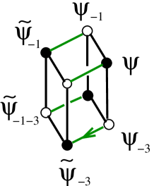
Figure 6. Geometry of the sublattice approach to the Darboux transformation of the linear problem on the honeycomb grid

Consider the wave function $\psi$ defined in the vertices of the hexahedron, like in Figure 6. The basic geometric property of the B-reduced fundamental transformation (see Remark 1.2) implies the possibility of eliminating the ”black points of the hexahedron” from the discrete Moutard equation

(4.20) $$\psi-\psi_{-1-3}=f^{13}_{-1-3}(\psi_{-3}-\psi_{-1}),$$

and the two Moutard transformation equations

(4.21) $$\tilde{\psi}-\psi_{-1} =\frac{\theta_{-1}}{\theta}(\tilde{\psi}_{-1}-\psi),$$

(4.22) $$\tilde{\psi}_{-3}-\psi_{-1-3} =\frac{\theta_{-1-3}}{\theta_{-3}}(\tilde{\psi}_{-1-3}-\psi_{-3}),$$

which gives

(4.23) $$\theta\tilde{\psi}-\theta_{-1-3}\tilde{\psi}_{-1-3}=f^{13}_{-1-3}(\theta_{-3}\psi_{-1}-\theta_{-1}\psi_{-3}).$$

Define $\check{\phi}^{+}=\theta_{-2-3}\tilde{\psi}_{-2-3}$, $\check{\phi}^{-}=\theta_{-1-3}\tilde{\psi}_{-1-3}$ in order to respect the duality transformation, and notice that $\theta^{+}=\theta_{1}$, $\theta^{-}=\theta_{2}$ are solutions of the honeycomb linear problem (2.11)-(2.12). In such notation, and taking into consideration equation (4.11), we can rewrite equation (4.23) in the form of the first equation (4.16) of the Darboux transformation system. A similar procedure gives equations

$$\theta_{-2-3}\tilde{\psi}_{-2-3}-\theta_{-1-3}\tilde{\psi}_{-1-3} =\frac{1}{f^{12}_{-1-2-3}}(\theta_{-3}\psi_{-1-2-3}-\theta_{-1-2-3}\psi_{-3}),$$

$$\theta_{-1-3}\tilde{\psi}_{-1-3}-\theta_{-1-2}\tilde{\psi}_{-1-2} =\frac{1}{f^{23}_{-1-2-3}}(\theta_{-1}\psi_{-1-2-3}-\theta_{-1-2-3}\psi_{-1}),$$

which, using equations (4.12), give the remaining part (4.17) and (4.18) of the Darboux tranformation system.

Because $\tilde{\psi}$ and $\theta^{-1}$ satisfy the same Moutard system, therefore $(\tilde{\psi}_{1},\tilde{\psi}_{2})$ and $(\theta^{-1}_{1},\theta^{-1}_{2})$ satisfy the same honeycomb affine linear system. By Corollary 2.4, the functions $(\check{\phi}^{+},\check{\phi}^{-})$ satisfy the honeycomb affine linear system, the coefficients of which can be found from equations (2.3) with $\tilde{f}^{ij}$ in place of $f^{ij}$, supplemented by the $(-1-2-3)$ shift and by the change (2.16) with respect to the above-mentioned gauge with $(\sigma^{+},\sigma^{-})=(\theta^{-1}_{-2-3},\theta^{-1}_{-1-3})$. This implies that the transformed coefficients read

$$\check{a} =\frac{\theta_{-2-3}\theta_{-1-3}}{\tilde{f}^{12}_{-1-2-3}}=\frac{\theta_{-3}\theta_{-1-2-3}}{f^{12}_{-1-2-3}},$$

$$\check{b} =\frac{\theta_{-1-2}\theta_{-1-3}}{\tilde{f}^{23}_{-1-2-3}}=\frac{\theta_{-1}\theta_{-1-2-3}}{f^{23}_{-1-2-3}},$$

$$\check{s}_{I,I\!I} =-\tilde{f}^{13}_{-1-3}\theta\theta_{-1-3}=-f^{13}_{-1-3}\theta_{-1}\theta_{-3},$$

which, using equations (4.11) and (4.12), take the form as in equation (4.19). ∎

5. Concluding remarks

We have derived the integrability properties of the self-adjoint linear problems on the triangular and honeycomb lattices from the well known theory of the 3D system of discrete Moutard equations. This result can be the starting point for several research programs. We would like to point out some of them.

In soliton theory, a linear problem admitting the Darboux type transformations can be used to construct evolution equations (with the time being discrete or continuous variable) compatible with the linear system; the standard example is the KdV hierarchy. As we have already remarked, the Laplace transformation equations (3.11)-(3.12) provide such a nonlinear system. More complicated evolutions of the triangular and honeycomb lattices are being studied, see [35].

Given integrable reduction of the 3D Moutard system (for example, the generalized isothermic lattice [15]), by restricting it to the quasiregular rhombic tiling one can obtain the corresponding integrable system on the triangular or on the honeycomb lattice. In particular, to obtain the constant angles circle patterns [5] one starts from further reduction of the generalized isothermic lattice. We remark, that such a process has already been built in the ”consistency around the cube” property [30, 4].

Finally, using the ”cut and project” method [39] in conjunction with the sublattice approach [21] one can derive linear problems (see also Remark 2.3) and integrable systems on more complicated graphs.

References

• [1] V. E. Adler, Legendre transforms on a triangular lattice, Funct. Anal. Appl. 34 (2000), 1–9.
• [2] V. E. Adler and Y. B. Suris, $Q_{4}$: integrable master equation related to an elliptic curve, Intern. Math. Research Notices 47 (2004) 2523–2553.
• [3] V.E. Adler and A.P. Veselov, Cauchy problem for integrable discrete equations on quad-graphs, Acta Applicandae Mathematicae 84 (2004), 237-262.
• [4] V. A. Adler, A. I. Bobenko, Yu. B. Suris, Classification of integrable equations on quad-graphs. The consistency approach, Commun. Math. Phys. 233 (2003), 513–543.
• [5] S. I. Agafonov and A. I. Bobenko, Hexagonal circle paterns with constant intersection angles and discrete Painlevé and Riccati equations, J. Math. Phys. 44 (2003), 3455-3469.
• [6] R. J. Baxter, Exactly solved models in statistical mechanics, Academic Press, London, 1982.
• [7] A. I. Bobenko, T. Hoffmann and Yu.B.Suris, Hexagonal circle patterns and integrable systems: Patterns with the multi-ratio property and Lax equations on the regular triangular lattice, Intern. Math. Research Notices 3 (2002), 111–164.
• [8] A. I. Bobenko and T. Hoffmann, Hexagonal circle patterns and integrable systems. Patterns with constant angles, Duke Math. J. (2003) 116, 525–566.
• [9] A. I. Bobenko and Yu. Suris, Integrable systems on quad-graphs, Internat. Math. Res. Notices 11 (2002), 573–611.
• [10] A. I. Bobenko, Ch. Mercat, Yu. B. Suris, Linear and nonlinear theories of discrete analytic functions. Integrable structure and isomonodromic Green’s function, J. Reine Angew. Math. 583 (2005) 117–161.
• [11] E. Date, M. Jimbo and T. Miwa, Method for generating discrete soliton equations. V, J. Phys. Soc. Japan 52 (1983), 766–771.
• [12] A. Doliwa, Geometric discretisation of the Toda system, Phys. Lett. A 234 (1997), 187–192.
• [13] A. Doliwa, Lattice geometry of the Hirota equation, [in:] SIDE III – Symmetries and Integrability of Difference Equations, D. Levi and O. Ragnisco (eds.), pp. 93–100, CMR Proceedings and Lecture Notes, vol. 25, AMS, Providence, 2000.
• [14] A. Doliwa, The B-quadrilateral lattice, its transformations and the algebro-geometric construction, J. Geom. Phys. 57 (2007), 1171–1192.
• [15] A. Doliwa, Generalized isothermic lattices, J. Phys. A: Math. and Theor. (to appear), (arXiv:nlin.SI/0611018).
• [16] A. Doliwa and P. M. Santini, Multidimensional quadrilateral lattices are integrable, Phys. Lett. A 233 (1997), 365–372.
• [17] A. Doliwa and P. M. Santini, The symmetric, D-invariant and Egorov reductions of the quadrilateral lattice, J. Geom. Phys. 36 (2000), 60–102.
• [18] A. Doliwa and P. M. Santini, Integrable systems and discrete geometry, [in:] Encyclopedia of Mathematical Physics, J. P. François, G. Naber and T. S. Tsun (eds.), Elsevier, 2006, Vol. III, pp. 78-87.
• [19] A. Doliwa, S. V. Manakov and P. M. Santini, $\bar{\partial}$-reductions of the multidimensional quadrilateral lattice: the multidimensional circular lattice, Comm. Math. Phys. 196 (1998), 1–18.
• [20] A. Doliwa, P. M. Santini and M. Mañas, Transformations of Quadrilateral Lattices, J. Math. Phys. 41 (2000) 944–990.
• [21] A. Doliwa, P. Grinevich, M. Nieszporski, and P. M. Santini, Integrable lattices and their sublattices: from the discrete Moutard (discrete Cauchy–Riemann) 4-point equation to the self-adjoint 5-point scheme, J. Math. Phys. 48 (2007), art. no. 013513 JAN 2007, doi: 10.1063/1.2406056.
• [22] I. A. Dynnikov and S. P. Novikov, Geometry of the triangle equations on two-manifolds, Mosc. Math. J. 3 (2003), 419–438.
• [23] R. Hirota, Discrete analogue of a generalized Toda equation, J. Phys. Soc. Jpn. 50 (1981), 3785–3791.
• [24] R. M. Kashaev, On discrete three-dimensional equation associated with the local Yang–Baxter relation, Lett. Math. Phys. 38 (1996), 389–397.
• [25] R. Kenyon, The Laplacian and Dirac operators on critical planar graphs, Invent. Math. 150 (2002), 409–439.
• [26] Ch. Mercat, Discrete Riemann surfaces and the Ising model, Commun. Math. Phys. 218 (2001), 177–216.
• [27] T. Miwa, On Hirota’s difference equations, Proc. Japan Acad. 58 (1982) 9–12.
• [28] M. Nieszporski, P. M. Santini and A. Doliwa, Darboux transformations for 5-point and 7-point self-adjoint schemes and an integrable discretization of the 2D Schrödinger operator, Phys. Lett. A 323 (2004), 241–250.
• [29] F. W. Nijhoff, Discrete Painlevé equations and symmetry reductions on the lattice, [in:] Discrete integrable geometry and physics, (A. Bobenko and R. Seiler, eds.), pp. 209–234, Clarendon Press, Oxford, 1999.
• [30] F. W. Nijhoff, Lax pair for the Adler (lattice Krichever–Novikov) system, Phys. Lett. A 297 (2002), 49–58.
• [31] J. J. C. Nimmo and W. K. Schief, Superposition principles associated with the Moutard transformation. An integrable discretisation of a (2+1)-dimensional sine-Gordon system, Proc. R. Soc. London A 453 (1997), 255–279.
• [32] S. P. Novikov, Difference analogs of Laplace transformations and two-dimensional Toda lattices, Appendix I in [33].
• [33] S. P. Novikov and A. P. Veselov, Exactly solvable two-dimensional Schrödinger operators and Laplace transformations, [in:] Solitons, geometry, and topology: on a crossroad, V. M. Buchstaber and S. P. Novikov (eds.) AMS Transl. 179 (1997), 109–132.
• [34] S. P. Novikov and I. A. Dynnikov, Discrete spectral symmetries of low dimensional differential operators and difference operators on regular lattices and two-dimensional manifolds, Russian Math. Surveys 52 (1997), 1057–1116.
• [35] P. M. Santini, A. Doliwa and M. Nieszporski, Integrable dynamics of Toda-type on the square and triangular lattices.
• [36] R. Sauer, Projective Liniengeometrie, de Gruyter, Berlin–Leipzig, 1937.
• [37] R. Sauer, Differenzengeometrie, Springer, Berlin, 1970.
• [38] J. Schiff, HexaKdV, arXiv:nlin.SI/0209041.
• [39] M. Senechal, Quasicrystals and geometry, Cambridge University Press, 1995.