When are Swing options bang-bang and how to use it?

Abstract

In this paper we investigate a class of swing options with firm constraints in view of the modeling of supply agreements. We show, for a fully general payoff process, that the premium, solution to a stochastic control problem, is concave and piecewise affine as a function of the global constraints of the contract. The existence of bang-bang optimal controls is established for a set of constraints which generates by affinity the whole premium function.

When the payoff process is driven by an underlying Markov process, we propose a quantization based recursive backward procedure to price these contracts. A priori error bounds are established, uniformly with respect to the global constraints.

Key words: Swing option, stochastic control, optimal quantization, energy.

1 Introduction

The deregulation of energy markets has given rise to various families of contracts. Many of them appear as some derivative products whose underlying is some tradable futures (day-ahead, etc) on gas or electricity (see [12] for an introduction). The class of swing options has been paid a special attention in the literature, because it includes many of these derivative products. A common feature to all these options is that they introduce some risk sharing between a producer and a trader, of gas or electricity for example. From a probabilistic viewpoint, they appear as some stochastic control problems modeling multiple optimal stopping problems (the control variable is the purchased quantity of energy); see $e.g.$ [10, 9] in a continuous time setting. Gas storage contracts (see [6], [8]) or electricity supply agreements (see [18], [7]) are examples of such swing options. Indeed, energy supply contracts are one simple and important example of such swing options that will be deeply investigated in this paper (see below, see also [12] for an introduction). It is worth mentioning that this kind of contracts are slightly different from multiple exercises American options as considered in [10] for example. In our setting the volumetric constraints play a key role and thus, the flexibility is not restricted to time decisions, but also has to take into account volumes management.

Designing efficient numerical procedures for the pricing of swing option contracts remains a very challenging question as can be expected from a possibly multi-dimensional stochastic control problem subject to various constraints (due to the physical properties of the assets like in storage contracts). Most recent approaches developed in mathematical finance, especially for the pricing of American options, have been adapted and transposed to the swing framework: tree (or “forest”) algorithms in the pioneering work [17], Least squares regression MC methods (see [6]), PDE’s numerical methods (finite elements, see [29]).

The aim of this paper is to deeply investigate an old question, namely to elucidate the structure of the optimal control in supply contracts (with firm constraints) and how it impacts the numerical methods of pricing. We will provide in a quite general (and abstract) setting some “natural” (and simple) conditions involving the local and global purchased volume constraints to ensure the existence of bang-bang optimal strategy (such controls usually do not exist). It is possible to design a priori the contract so that their parameters satisfy these conditions. To our knowledge very few theoretical results have been established so far on this problem (see however [6] in a Markovian framework for contracts with penalized constraints and [27], also in a Markovian framework).

This first result of the paper not only enlightens the understanding of the management of a swing contract: it also has some deep repercussions on the numerical methods to price it. As a matter of fact, taking advantage of the existence of a bang-bang optimal strategy, we propose and analyze in details (when the underlying asset has a Markovian dynamics) a quantized Dynamic Programming procedure to price any swing options whose volume constraints satisfy the “bang-bang” assumption. Furthermore some a priori error bounds are established. This procedure turns out to be dramatically efficient, as emphasized in the companion paper [5] where the method is extensively tested with assets having multi-factor Gaussian underlying dynamics and compared to the least squares regression method.

The abstract swing contract with firm constraints

The holder of a supply contract has the right to purchase periodically (daily, monthly, etc) an amount of energy at a given unitary price. This amount of energy is subject to some lower and upper “local” constraints. The total amount of energy purchased at the end of the contract is also subject to a “global” constraint. Given dynamics on the energy price process, the problem is to evaluate the price of such a contract, at time $t=0$ when it is emitted and during its whole life up to its maturity.

To be precise, the owner of the contract is allowed to purchase at times $t_{i}$, $i=0,\ldots,n-1$ a quantity $q_{i}$ of energy at a unitary strike price $K_{i}:=K(t_{i})$. At every date $t_{i}$, the purchased quantity $q_{i}$ is subject to the firm “local” constraint,

$$q_{\min}\leq q_{i}\leq q_{\max},\qquad i=0,\ldots,n-1,$$

whereas the global purchased quantity $\bar{q}_{n}:=\sum_{i=0}^{n-1}q_{i}$ is subject to the (firm) global constraint

$$\bar{q}_{n}\!\in[Q_{\min},Q_{\max}]\qquad(0<Q_{\min}\leq Q_{\max}<+\infty).$$

The strike price process $(K_{i})_{0\leq i\leq n-1}$ can be either deterministic (even constant) or stochastic, $e.g.$ indexed on past values of other commodities (oil, etc). Usually, on energy markets the price is known through future contracts $(F_{s,t})_{0\leq s\leq t}$ where $F_{s,t}$ denotes the price at time $s$ of the forward contract delivered at maturity $t$. The available data at time $0$ are $(F_{0,t})_{0\leq t\leq T}$ (in real markets this is of course not a continuum).

The underlying asset price process, temporarily denoted $(S_{t_{i}})_{0\leq i\leq n-1}$, is often the so-called “day-ahead” contract $F_{t,t+1}$ which is a tradable instrument or the spot price $F_{t,t}$ which is not. All the decisions about the contract need to be adapted to the filtration of $(S_{t_{i}})$ $i.e.$ ${\cal F}_{i}:=\sigma(S_{t_{j}},j=0,\ldots,i)$, $i=0,\ldots,n-1$ (with ${\cal F}_{0}=\{\emptyset,\Omega\}$). This means that the price of such a contract is given at any time $t_{k}$, by

$$P^{n}_{k}(Q^{k}_{\min},Q^{k}_{\max}) := {\rm esssup}\left\{{E}\left(\sum_{j=k}^{n-1}\!q_{j}e^{-r(t_{j}-t_{k})}(S_{t_{j}}-K_{j})\,|\,{\cal F}_{k}\right),\right.$$

$$\left.q_{j}:(\Omega,{\cal F}_{j})\to[q_{\min},q_{\max}],j=k,\ldots,n-1,\sum_{j=k}^{n-1}q_{j}\!\in[Q^{k}_{\min},Q^{k}_{\max}]\right\}$$

where $Q^{k}_{\min}=Q_{\min}-\bar{q}_{k}$, $Q^{k}_{\max}=Q_{\max}-\bar{q}_{k}$ denote the residual global constraints and $r$ denotes the (deterministic) interest rate. This pricing problem clearly appears as a stochastic control problem.

In the pioneering work by [17], this type of contract was computed by using some forests of (multinomial) trees. A natural variant, at least for numerical purpose, is to consider a penalized version of this stochastic control. Thus, in [6], a penalization $Q_{n}(V_{n},\bar{q}_{n})$ with $Q_{n}(x,q)=-((x-Q_{\max})^{+}+(x-Q_{\min})^{+})/\varepsilon$ is added ($Q_{n}$ is negative outside $[Q_{\min},Q_{\max}]$ and zero inside).

As concerns more sophisticated contracts (like storages), the holder of the contract receive a quantity $\Psi(t_{i},S_{t_{i}},q_{i})$ when deciding $q_{i}$. When dealing with gas this is due to the storing constraints since injecting or withdrawing gas from its storing units induce fixed costs (and physical constraints (pressure, etc)).

As concerns the underlying asset dynamics, it is commonly shared in finance to assume that the traded asset has a Markovian dynamics (or is a component of a Markov process like with stochastic volatility models). The dynamics of physical assets for many reasons (some of them simply coming from history) are often modeled using some more deeply non-Markovian models like long memory processes, etc.

All these specific features of energy derivatives suggest to tackle the above pricing problem in a rather general framework, trying to avoid as long as possible to call upon Markov properties. This is what we do in the first part of the paper where the general setting of a swing option defined by an abstract sequence of ${\cal F}_{k}$-adapted payoffs is deeply investigated as a function of its global constraints $(Q_{\min},Q_{\max})$ (when the local constraints are normalized $i.e.$ $q_{i}$ is $[0,1]$-valued for every $i\!\in\{0,\ldots,n-1\}$). We show that this premium is a concave, piecewise affine, function of the global constraints, affine on triangles of the $(m,M)+\{(u,v),\;0\leq u\leq v\leq 1\}$, $m,\,M\!\in{N}^{2}$, $m\leq M\leq n$ and $(m,M)+\{(u,v),\;0\leq v\leq u\leq 1\}$, $m,\,M\!\in{N}^{2}$, $m\leq M-1\leq n-1$. We also show that for integral valued global constraints, the optimal controls are always bang-bang $i.e.$ the a priori $[0,1]$-valued optimal purchased quantities $q^{*}_{i}$ are in fact always equal to $0$ or $1$. Such a result can be extended in some way to any couple of global constraints when all the payoffs are nonnegative.

Then, when there is an underlying Markov “structure process”, we propose an optimal quantization based on numerical approach to price efficiently swing options. This Markov “structure process” can be the underlying traded asset itself or a higher dimensional hidden Markov process: such a framework comes out in case of multi-factor processes having some long-memory properties.

Optimal Quantization was first introduced as a numerical method to solve nonlinear problem arising in Mathematical Finance in a series of papers [1, 2, 3, 4] devoted to the pricing and hedging of American style multi-asset options. It has also been applied to stochastic control problem, namely portfolio optimization in [24]. The purely numerical aspects induced by optimal quantization, with a special emphasis on the Gaussian distribution, have been investigated in [26]. See [25] for a survey on numerical application of optimal quantization to Finance. For other applications (to automatic classification, clustering, etc), see also [14]. In this paper, we propose a quantized backward dynamic programming to approximate the premium of a swing contract. We analyze the rate of convergence of this algorithm and provide some a priori error bounds in terms of quantization errors.

We illustrate the method by computing the whole graph of the premium viewed as a function of the global constraints, combining the affine property of the premium and the quantized algorithm in “toy model”: the future prices of gas are modeled by a two factor Gaussian model. An extensive study of the pricing method by optimal quantization is carried out from both a theoretical and numerical point of view in [5].

The paper is organized as follows. In the section below we detail the decomposition of swing options into a swap contract and a normalized swing option. In Section 3, we precisely describe our abstract setting for normalized swing options with firm constraints and the variable of interest (global constraints, local constraints, etc). In Section 4, we establish the dynamic programming formula satisfied in full generality by the premium as a function of the global constraints (this unifies the similar results obtained in Markov settings, see [17], [6], etc) and we show this is a concave function with respect to the global constraints. Then, in Section 5, we prove in our abstract framework that the premium function is piecewise affine and that the optimal purchased quantities satisfy a “$0$-$1$” or bang-bang principle (Theorem 2). A special attention is paid to the $2$-period model which provides an intuitive interpretation of the results. In Section 6, after some short background on quantization and its optimization, we propose a quantization based backward dynamic programming formula as a numerical method to solve the swing pricing problem. Then we provide some error bounds for the procedure depending on the quantization error induced by the quantization of the Markov structure process.

Notations. $\bullet$ The Lipschitz coefficient of a function $f:{R}^{d}\to{R}$ is defined by $\displaystyle[f]_{\rm Lip}:=\sup_{x\neq y}\frac{|f(x)-f(y)|}{|x-y|}\leq+\infty$. The coefficient $[f]_{\rm Lip}$ is finite if and only if $f$ Lipschitz continuous.

$\bullet$ The canonical Euclidean norm on ${R}^{d}$ will be denoted $|\,.\,|$.

2 Canonical decomposition, normalized swing option

As a first step we need to normalize this contract to reduce some useless technical aspects. In practice this normalization, in fact decomposition, corresponds to the splitting of the contract into a swap and a normalized swing. The decomposition can be derived from the fact that an ${\cal A}$-measurable random variable $q$ is $[q_{\min},q_{\max}]$-valued if and only if there exists a $[0,1]$-valued ${\cal A}$-measurable random variable $q^{\prime}$ such that $q=q_{\min}+(q_{\max}-q_{\min})q^{\prime}$. Then, for every $k\!\in\{0,\ldots,n-1\}$,

$$P^{n}_{k}(Q^{k}_{\min},Q^{k}_{\max}) = q_{\min}\underbrace{\sum_{j=k}^{n-1}\!e^{-r(t_{j}-t_{k})}{E}(S_{t_{j}}-K_{j}\,|\,{\cal F}_{k})}_{\mbox{\em swap contract}}+(q_{\max}-q_{\min})\!\underbrace{P^{[0,1],n}_{k}\left(\widetilde{Q}^{k}_{\min},\widetilde{Q}^{k}_{\max}\right)}_{\mbox{\em normalized contract}}$$

where

$$\widetilde{Q}^{k}_{\min}=\frac{Q^{k}_{\min}-(n-k)q_{\min}}{q_{\max}-q_{\min}}\qquad\mbox{ and }\qquad\widetilde{Q}^{k}_{\max}=\frac{Q^{k}_{\max}-(n-k)q_{\min}}{q_{\max}-q_{\min}}$$

and $P^{[0,1],n}_{k}\left(\widetilde{Q}^{k}_{\min},\widetilde{Q}^{k}_{\max}\right)$ is a normalized swing contract in which the local constraints are $[0,1]$-valued .

3 An abstract model for swing options with firm constraints

One considers a sequence $(V_{k})_{0\leq k\leq n-1}$ of integrable random variables defined on a probability space $(\Omega,{\cal A},{P})$. Let ${\cal F}_{k}^{V}:=\sigma(V_{0},V_{1},\ldots,V_{k}),\;k=0,\ldots,n-1$ denote its natural filtration. For convenience we introduce a more general discrete time filtration ${\cal F}:=({\cal F}_{k})_{0\leq k\leq n-1}$ to which $V=(V_{k})_{0\leq k\leq n-1}$ is adapted $i.e.$ satisfying ${\cal F}_{k}^{V}\subset{\cal F}_{k}$, $k=0,\ldots,n-1$ $i.e.$ such that the sequence $(V_{k})_{0\leq k\leq n-1}$ is ${\cal F}$-adapted.

We aim to solve the following abstract stochastic control problem (with maturity $n$)

$$({\cal S})^{\cal F}_{n}\equiv{\rm esssup}\left\{{E}\left(\sum_{k=0}^{n-1}\!q_{k}V_{k}\,|\,{\cal F}_{0}\right),\;q_{k}:(\Omega,{\cal F}_{k})\to[0,1],0\leq k\leq\ldots,n-1,\sum_{k=0}^{n-1}q_{k}\!\in[Q_{\min},Q_{\max}]\right\}$$ (3.1)

where $Q_{\min}$ and $Q_{\max}$ are two non-negative ${\cal F}_{0}$-measurable random variables satisfying

$$0\leq Q_{\min}\leq Q_{\max}\leq n.$$ (3.2)

(The inequality $Q_{\max}\leq n$ induces no loss of generality: one can always replace $Q_{\max}$ by $Q_{\max}\wedge n$ in (3.1) since in any case $q_{0}+\dots+q_{n}\leq n$).

Note that no assumption is made on the dynamics of the state process $V=(V_{k})_{0\leq k\leq n-1}$.

We need to introduce the following notations and terminology:

– Throughout the paper, ${\rm esssup}$ will always be taken with respect to the probability ${P}$ so ${P}$ will be dropped from now on.

– A couple $Q:=(Q_{\min},Q_{\max})$ of non-negative ${\cal F}_{k}$-measurable random variables satisfying $0\leq Q_{\min}\leq Q_{\max}\leq n\!-\!k$ is called a couple of global constraints at time $k$.

– An ${\cal F}$-adapted sequence $q=(q_{k})_{0\leq k\leq n-1}$ of $[0,1]$-valued r.v. is called a locally admissible control. For any locally admissible control, one defines the cumulative purchase process by

$$\bar{q}_{0}:=0,\quad\bar{q}_{k}:=q_{0}+\cdots+q_{k-1},\;k=1,\ldots,n.$$

If $\bar{q}_{n}\!\in[Q_{\min},Q_{\max}]$, $q$ is called an $({\cal F},Q)$-admissible control.

– For every $k\!\in\{0,\ldots,n\}$ and every couple of global constraints $Q:=(Q_{\min},Q_{\max})$ at time $k$, set

$$P^{n}_{k}(Q,(V,{\cal F})):={\rm esssup}\left\{{E}\left(\sum_{\ell=k}^{n-1}q_{\ell}V_{\ell}\,|\,{\cal F}_{k}\right),\;q\;({\cal F},Q)\mbox{-admissible control}\right\}$$ (3.3)

so that $P^{n}_{0}(Q,(V,{\cal F}))$ is the value function of the stochastic control problem (3.1) when the global constraints $Q_{\min}$ and $Q_{\max}$ (at time $0$) satisfy (3.2). Note that the standard convention ${\rm esssup}(\o)=0$ yields $P^{n}_{n}\equiv 0$. To alleviate notations, the payoff process $V$ the filtration ${\cal F}$ will be often dropped in $P^{n}_{k}(Q,(V,{\cal F}))$.

To be precise we will answer the following questions:

$\bullet$ Existence of an optimal control $q^{*}=(q^{*}_{k})_{0\leq k\leq n-1}$.

$\bullet$ Regularity of the value function $Q\mapsto P^{n}_{k}(Q,(V,{\cal F}))$.

$\bullet$ Existence of a bang-bang optimal control $(q^{*}_{k})_{0\leq k\leq n-1}$ for certain values of the global constraints $Q$ (namely when $Q$ has integral components) ?

By bang-bang we mean that ${P}(d\omega)$-$a.s.$

– all the local constraints on the $q_{k}(\omega)$ are saturated $i.e.$ for every $k\!\in\{0,\ldots,n-1\}$, $q_{k}(\omega)\!\in\{0,1\wedge Q_{\max}\}$

or

– there exists at most one instant $k_{0}(\omega)$ such that $q_{k_{0}(\omega)}(\omega)\!\in(0,1\wedge Q_{\max})$ and one global constraint is saturated.

Note that if $Q\!\in{N}^{2}$, then a bang-bang $Q$-admissible control necessary satisfies ${P}(d\omega)$-$a.s.$ $q_{k}(\omega)\!\in\{0,1\}$, $k=0,\ldots,n-1$. The existence of bang-bang optimal controls combined with the piecewise affinity of $P^{n}_{k}(Q)$ will be the key in the design of a numerical.

$\bullet$ When there is an underlying structure Markov process ($V_{k}=v_{k}(Y_{k}))$, we will show that the optimal control turns out to be a function of $Y_{k}$ at every time $k$ as well.

4 Abstract dynamical programming principle and first properties

4.1 Basic properties

As a first step, we need to establish the following easy properties of $P^{n}_{k}$ as a function of the global constraints $Q=(Q_{\min},Q_{\max})$.

P1. For every $k\!\in\{0,\ldots,n\}$, and every couple of global constraints (at time $k$),

$$P^{n}_{k}(Q,(V_{k},{\cal F}_{k})_{0\leq k\leq n-1})=P_{0}^{n\!-\!k}(Q,(V_{k+\ell},{\cal F}_{k+\ell})_{0\leq\ell\leq n\!-\!k-1}).$$

This is obvious from (3.3).

P2. If $Q$ and $Q^{\prime}$ are two admissible global constraints (at time $k$) then

$$P^{n}_{k}(Q)=P^{n}_{k}(Q^{\prime})\quad\mbox{ on the event }\quad\{Q=Q^{\prime}\}.$$

Proof. Owing to P1 one may assume without loss of generality that $k=0$. Let $q$ and $q^{\prime}$ be two admissible controls with respect to $Q$ and $Q^{\prime}$ respectively. Set $\tilde{q}_{\ell}=q_{\ell}\mbox{\bf 1}_{\{Q=Q^{\prime}\}}+q^{\prime}_{\ell}\mbox{\bf 1}_{\{Q\neq Q^{\prime}\}}$, $\ell=0,\ldots,n-1$. The control $\tilde{q}$ is admissible with respect to $Q^{\prime}$ since $\{Q=Q^{\prime}\}\!\in{\cal F}_{0}$. Furthermore,

$$\mbox{\bf 1}_{\{Q=\ Q^{\prime}\}}{E}\left(\sum_{\ell=0}^{n-1}q_{\ell}V_{\ell}\,|\,{\cal F}_{0}\right)\! \!=\! \!{E}\left(\sum_{\ell=0}^{n-1}\mbox{\bf 1}_{\{Q=Q^{\prime}\}}q_{\ell}V_{\ell}\,|\,{\cal F}_{0}\right)=\mbox{\bf 1}_{\{Q=Q^{\prime}\}}{E}\left(\sum_{\ell=0}^{n-1}\widetilde{q}_{\ell}V_{\ell}\,|\,{\cal F}_{0}\right).$$

$$\leq \mbox{\bf 1}_{\{Q=Q^{\prime}\}}P^{n}_{0}(Q^{\prime})\quad a.s.$$

Hence,

$$\mbox{\bf 1}_{\{Q=Q^{\prime}\}}P^{n}_{0}(Q)={\rm esssup}\left\{\mbox{\bf 1}_{\{Q=Q^{\prime}\}}{E}\left(\sum_{\ell=0}^{n-1}q_{\ell}V_{\ell}\,|\,{\cal F}_{0}\right),\;q\hbox{ $Q$-admissible}\right\}\leq\mbox{\bf 1}_{\{Q=Q^{\prime}\}}P^{n}_{0}(Q^{\prime})\quad a.s.$$

The equality follows by symmetry.$\quad{}_{\diamondsuit}$

P3. Let $k\!\in\{0,\ldots,n-1\}$. The set of admissible global constraints $Q=(Q_{\min},Q_{\max})$ at time $k$ is convex and the mapping $Q\mapsto P^{n}_{k}(Q)$ is concave in the following sense: if $Q$ and $Q^{\prime}$ are two couples of admissible constraints, then for every random variable $\lambda:(\Omega,{\cal F}_{k})\to[0,1]$, $\lambda Q+(1-\lambda)Q^{\prime}$ is an admissible couple of constraints and

$$P^{n}_{k}(\lambda Q+(1-\lambda)Q^{\prime})\geq\lambda P^{n}_{k}(Q)+(1-\lambda)P^{n}_{k}(Q^{\prime})\quad a.s.$$

Furthermore $Q_{\min}\mapsto P^{n}_{k}(Q_{\min},Q_{\max})$ is non-increasing and $Q_{\max}\mapsto P^{n}_{k}(Q_{\min},Q_{\max})$ is non-decreasing $i.e.$

$$P^{n}_{k}(Q)\leq P^{n}_{k}(Q^{\prime})\qquad a.s.\qquad\mbox{\rm on }\quad\{Q^{\prime}_{\min}\leq Q_{\min}\leq Q_{\max}\leq Q^{\prime}_{\max}\}.$$

Proof. One may assume by P1 that $k=0$. The convexity of admissible global constraints is obvious. As concerns the concavity of the value function, note that if $q$ and $q^{\prime}$ are locally admissible controls then $\lambda q+(1-\lambda)q^{\prime}:=(\lambda q_{k}+(1-\lambda)q^{\prime}_{k})_{0\leq k\leq n-1}$ is still locally admissible. If $q$ and $q^{\prime}$ satisfy the global constraints induced by $Q$ and $Q^{\prime}$ respectively, then $\lambda q+(1-\lambda)q^{\prime}$ always satisfies that induced by $\lambda Q+(1-\lambda)Q^{\prime}$. Consequently, using that $\lambda$ is ${\cal F}_{0}$-measurable,

$$P^{n}_{0}(\lambda Q+(1-\lambda)Q^{\prime})$$

$$\geq {\rm esssup}\left\{{E}(\sum_{k=0}^{n-1}(\lambda q_{k}+(1-\lambda)q^{\prime}_{k})V_{k}\,|\,{\cal F}_{0}),\,q,\,q^{\prime}\hbox{ locally admissible},\,\bar{q}_{n}\!\in[Q_{\min},Q_{\max}],\,\bar{q}^{\prime}_{n}\!\in[Q^{\prime}_{\min},Q^{\prime}_{\max}]\right\}$$

$$\!=\! \!\lambda\,{\rm esssup}\left\{{E}(\sum_{k=0}^{n-1}q_{k}V_{k}\,|\,{\cal F}_{0}),\,q\hbox{ locally admissible},\,\bar{q}_{n}\!\in[Q_{\min},Q_{\max}]\right\}$$

$$+(1-\lambda)\,{\rm esssup}\left\{{E}(\sum_{k=0}^{n-1}q^{\prime}_{k}V_{k}\,|\,{\cal F}_{0}),\,q^{\prime}\hbox{ locally admissible},\,\bar{q}^{\prime}_{n}\!\in[Q^{\prime}_{\min},Q^{\prime}_{\max}]\right\}$$

$$\!=\! \!\lambda P^{n}_{0}(Q)+(1-\lambda)P^{n}_{0}(Q^{\prime}).$$

The monotony property is as follows: let $A:=\{Q^{\prime}_{\min}\leq Q_{\min}\leq Q_{\max}\leq Q^{\prime}_{\max}\}\!\in{\cal F}_{0}$ and let $\tilde{q}^{\prime}$ be a fixed $Q^{\prime}$-admissible control. Then, for every $Q$-admissible control $q$, set

$$q^{\prime}:=q\mbox{\bf 1}_{{}_{A}}+\tilde{q}^{\prime}\mbox{\bf 1}_{{}^{c}A}.$$

Then $q^{\prime}$ is clearly $Q^{\prime}$-admissible and

$$\mbox{\bf 1}_{{}_{A}}{E}\left(\sum_{k=0}^{n-1}q_{k}V_{k}\,|\,{\cal F}_{0}\right) = {E}\left(\sum_{k=0}^{n-1}\mbox{\bf 1}_{{}_{A}}q_{k}V_{k}\,|\,{\cal F}_{0}\right)$$

$$= {E}\left(\mbox{\bf 1}_{{}_{A}}\sum_{k=0}^{n-1}q^{\prime}_{k}V_{k}\,|\,{\cal F}_{0}\right)$$

$$\leq \mbox{\bf 1}_{{}_{A}}P_{0}^{n}(Q^{\prime})\qquad a.s.$$

$$\mbox{ so that }\hskip 142.26378pt\mbox{\bf 1}_{{}_{A}}P^{n}_{0}(Q) \leq \mbox{\bf 1}_{{}_{A}}P^{n}_{0}(Q^{\prime})\qquad a.s.\hskip 64.01869pt\qquad\quad_{\diamondsuit}$$

P4. Let $k\!\in\{0,\ldots,n-1\}$. Let $Q^{(n)}$, $n\geq 1$, be a sequence of admissible global constraints such that $Q^{(n)}_{\max}\to 0$ as $n\to\infty$. Then

$$P_{k}^{n}(Q^{(n)})\longrightarrow 0\qquad\mbox{ as }\qquad n\to\infty.$$

Proof. Owing to P1, one may assume $k=0$ without loss of generality. The result is straightforward once noticed that for every $Q$-admissible control

$$\left|{E}\left(\sum_{k=0}^{n-1}q_{k}V_{k}\,|\,{\cal F}_{0}\right)\right|\leq Q_{\max}{E}\left(\max_{0\leq k\leq n-1}|V_{k}|\,|\,{\cal F}_{0}\right).\qquad\quad_{\diamondsuit}$$

P5. Let $T^{+}(n):=\{(u,v)\!\in{R}_{+}^{2},\,0\leq u\leq v\leq n\}$ and let $k\!\in\{0,\ldots,n-1\}$. There is process $\Pi^{n}_{k}:(T^{+}(n)\times\Omega,{\cal B}or(T^{+}(n))\otimes{\cal F}_{k})\to{R}$ such that

$(i)$ $(u,v)\mapsto\Pi^{n}_{k}(u,v,\omega)$ is concave and continuous on $T^{+}(n)$ for every $\omega\!\in\Omega$,

$(ii)$ $u\mapsto\Pi^{n}_{k}(u,v,\omega)$ is non-increasing on $[0,v]$ and $v\mapsto\Pi^{n}_{k}(u,v,\omega)$ is nondecreasing on $[u,n]$ for every $\omega\!\in\Omega$.

$(iii)$ For every admissible constraint $Q=(Q_{\min},Q_{\max})$ at time $k$, $P^{n}_{k}(Q)(\omega)=\Pi^{n}_{k}(Q(\omega),\omega)$ ${P}(d\omega)$-$a.s.$

Proof. Classical consequence of P3: for every $(r,s)\!\in T^{+}(n)\cap{Q}^{2}$ set

$$\Pi^{n}_{k}((r,s),\omega):=P^{n}_{k}((r,s))(\omega).$$

Then, set for every $(u,v)\!\in T^{+}(n)$

$$\Pi^{n}_{k}((u,v),\omega):=a.s.\lim_{(r,s)\to(u,v),(r,s)\in T^{+}(n)\cap{Q}^{2},r\leq u\leq v\leq s}P^{n}_{k}((r,s))(\omega).$$

One shows using the concavity and monotony properties established in P3 that the above limit does exist and that , ${P}(d\omega)$-$a.s.$ $(u,v)\mapsto\Pi^{n}_{k}((u,v),\omega)$ is continuous on $T^{+}(n)$ and that $P^{n}_{k}(Q)(\omega)=\Pi^{n}_{k}(Q(\omega),\omega)$ ${P}$-$a.s.$.

P6. Let $Q=(Q_{\min},Q_{\max})$ be a couple of global constraints (at time $0$).

$$P^{n}_{0}(Q)={\rm esssup}\left\{{E}\left(\sum_{\ell=0}^{n-1}q_{\ell}(V_{\ell})^{+}\,|\,{\cal F}_{0}\right),\;q\hbox{ $({{\cal F}},Q)$-admissible}\right\}\;\mbox{ on the event }\;\{Q_{\min}=0\}\!\in{\cal F}_{0}.$$

Proof. This follows from the simple remark that one can define from any $({{\cal F}},Q)$-admissible control $q$ a new $({{\cal F}},Q)$-admissible control $\widetilde{q}$ by $\widetilde{q}_{\ell}:=q_{\ell}\mbox{\bf 1}_{\{V_{\ell}\geq 0\}\cap\{Q_{\min}=0\}}+q_{\ell}\mbox{\bf 1}_{\{Q_{\min}>0\}}$ and

$$\mbox{\bf 1}_{\{Q_{\min}=0\}}\sum_{k=0}^{n-1}q_{\ell}V_{\ell}\leq\mbox{\bf 1}_{\{Q_{\min}=0\}}\sum_{k=0}^{n-1}q_{\ell}(V_{\ell})^{+}=\mbox{\bf 1}_{\{Q_{\min}=0\}}\sum_{k=0}^{n-1}\tilde{q}_{\ell}(V_{\ell})^{+}.\quad_{\diamondsuit}$$

4.2 Dynamic programming principle

The main consequence of P5 is that at every time $k$, one may assume without loss of generality that the couple of admissible global constraints $Q=(Q_{\min},Q_{\max})$ is deterministic since, for any possibly random admissible constraint $Q$ (at time $k$) and every $\omega\!\in\Omega$, $P^{n}_{k}(Q)(\omega)=\Pi^{n}_{k}(\omega,Q(\omega))$.

As a consequence, for notational convenience, we will still denote $P^{n}_{k}$ instead of $\Pi^{n}_{k}$ so that for any admissible global constraints $Q$ at time $k$

$$P^{n}_{k}(Q)(\omega)=P^{n}_{k}(\omega,x)_{|x=Q(\omega)}.$$

Theorem 1

(Backward Dynamic Programming Principle) Set $P^{n}_{n}\equiv 0$.

$(a)$ Local Dynamic programming formula. For every $k\!\in\{0,\ldots,n-1\}$ and every couple $Q=(Q_{\min},Q_{\max})$ of deterministic admissible global constraints at time $k$

$$\hskip-9.95863ptP^{n}_{k}(Q)=\sup\left\{xV_{k}+{E}\left(P^{n}_{k+1}(\chi^{n\!-\!k-1}(Q,x))\,|\,{\cal F}_{k}\right),\,x\!\in I^{n-1-k}_{Q}\right\}$$ (4.1)

where $\chi^{M}(Q,x)=((Q_{\min}-x)^{+},(Q_{\max}-x)\!\wedge\!M)$ and $I^{M}_{Q}:=[(Q_{\min}-M)^{+}\!\wedge\!1,Q_{\max}\!\wedge\!1]$.

$(b)$ Global Dynamic programming formula. For every couple $Q=(Q_{\min},Q_{\max})$ of admissible global constraints at time $0$, the price of the contract at time $k\!\in\{0,\ldots,n-1\}$ is given by $P^{n}_{k}(Q^{k,*})$ where

$$Q^{k,*} := (Q_{\max}-\bar{q}^{*}_{k},Q_{\min}-\bar{q}^{*}_{k})\hskip 28.45274pt\mbox{(residual global constraints) }$$ (4.2)

$$\mbox{with }\hskip 22.76228ptq^{*}_{k} = q^{*}_{k}(Q^{k,*})\hskip 142.26378pt$$

$$q^{*}_{k}(Q) := {\rm argmax}_{x\in I^{n-1-k}_{Q}}\left(xV_{k}+{E}\left(P^{n}_{k+1}(\chi^{n-k-1}(Q,x))\,|\,{\cal F}_{k}\right)\right),\;k=0,\ldots,n-1.\qquad$$ (4.3)

Furthermore,

$$P^{n}_{k}(Q^{k,*})={E}\left(\sum_{\ell=k}^{n-1}q^{*}_{\ell}V_{\ell}\,|\,{\cal F}_{\ell}\right).$$

Remark. The definition (4.3) may be ambiguous when argmax is not reduced to a single point. Then, one considers $\min\,$argmax to define $q^{*}_{k}(Q)$.

Proof. $(a)$ It is clear that owing to P1 the case $k=0$ is the only one to be proved. As a first step, we prove that

$$\hskip-9.95863ptP^{n}_{0}(Q)={\rm esssup}\left\{q_{0}V_{0}+{E}\left(P^{n}_{1}(\chi^{n-1}(Q,q_{0}))\,|\,{\cal F}_{0}\right),\,q_{0}:(\Omega,{\cal F}_{0})\to I^{n-1}_{Q}\right\}$$ (4.4)

$\leq$ : Let $q=(q_{k})_{0\leq k\leq n-1}$ be a $Q$-admissible control. Then, $q_{0}$ is $[0,1]$-valued (as well as the $q_{k}$’s) and

$$Q_{\min}-(n-1)\leq Q_{\min}-(q_{1}+\cdots+q_{n-1})\leq q_{0}\leq Q_{\max}-(q_{1}+\cdots+q_{n-1})\leq Q_{\max}$$

so that $q_{0}$ is $I^{n-1}_{Q}$-valued. Furthermore,

$$\max(0,Q_{\min}-q_{0})\leq q_{1}+\cdots+q_{n-1}\leq(Q_{\max}-q_{0})\!\wedge\!(n-1).$$ (4.5)

note that $\chi^{n-1}(Q,q_{0})$ is an admissible couple of (${\cal F}_{0}$-measurable) constraints at time $1$. Consequently,

$${E}\left(\sum_{1\leq\ell\leq n-1}q_{\ell}V_{\ell}\,|\,{\cal F}_{0}\right)\! \!=\! \!{E}\left({E}\left(\sum_{1\leq\ell\leq n-1}q_{\ell}V_{\ell}\,|\,{\cal F}_{1}\right)\,|\,{\cal F}_{0}\right)$$

$$\leq {E}\left(P^{n}_{1}(\chi^{n-1}(Q,q_{0}))\,|\,{\cal F}_{0}\right)\quad a.s.$$

where the last inequality follows from the definition of $P^{n}_{1}$, $\chi^{n-1}$, (4.5) and the monotony of conditional expectation. Then,

$${E}\left(\sum_{0\leq\ell\leq n-1}q_{\ell}V_{\ell}\,|\,{\cal F}_{0}\right)\leq{E}\left(q_{0}V_{0}+P^{n}_{1}(\chi^{n-1}(Q,q_{0}))\,|\,{\cal F}_{0}\right)\quad a.s.$$

One concludes that

$$P^{n}_{0}(Q)\leq{\rm esssup}\left\{{E}\left(q_{0}V_{0}+P^{n}_{1}(\chi^{n-1}(Q,q_{0}))\,|\,{\cal F}_{0}\right),\;q_{0}:(\Omega,{\cal F}_{0})\to I^{n-1}_{Q}\right\}.$$

$\geq$ : We proceed as usual by proving a bifurcation property for the controls. Let $q_{0}$ and $q^{\prime}_{0}$ be two $I^{n-1}_{Q}$-valued ${\cal F}_{0}$-measurable random variables. Set

$$A_{0}:=\left\{q_{0}V_{0}+{E}\left(P^{n}_{1}(\chi^{n-1}(Q,q_{0}))\,|\,{\cal F}_{0}\right)>q^{\prime}_{0}V_{0}+{E}\left(P^{n}_{1}(\chi^{n-1}(Q,q^{\prime}_{0}))\,|\,{\cal F}_{0}\right)\right\}\!\in{\cal F}_{0}.$$

and

$$\tilde{q}_{0}=q_{0}\mbox{\bf 1}_{A_{0}}+q^{\prime}_{0}\mbox{\bf 1}_{{}^{c}A_{0}}:(\Omega,{\cal F}_{0})\to I^{n-1}_{Q}.$$

Then, one checks that

$$\tilde{q}_{0}V_{0}+{E}\left(P^{n}_{1}(\chi^{n-1}(Q,\tilde{q}_{0}))|{\cal F}_{0}\right)=\max_{y=q_{0},q^{\prime}_{0}}\left(yV_{0}+{E}\left(P^{n}_{1}(\chi^{n-1}(Q,y))|{\cal F}_{0}\right)\right).$$

Consequently there exists a sequence $q_{0}^{(n)}$ of $[0,Q_{\max}\wedge 1]$-valued random variables such that

$${\rm esssup}\left\{q_{0}V_{0}+{E}\left(P^{n}_{1}(\chi^{n-1}(Q,q_{0}))\,|\,{\cal F}_{0}\right),\,q_{0}:(\Omega,{\cal F}_{0})\to I^{n-1}_{Q}\right\}$$

$$=\sup_{n}q^{(n)}_{0}V_{0}+{E}\left(P^{n}_{1}(\chi^{n-1}(Q,q^{(n)}_{0}))\,|\,{\cal F}_{0}\right)$$

$$=\lim^{\;\qquad{}_{\uparrow}}_{n}q^{(n)}_{0}V_{0}+{E}\left(P^{n}_{1}(\chi^{n-1}(Q,q^{(n)}_{0}))\,|\,{\cal F}_{0}\right).$$

One may assume by applying the above bifurcation property that the above supremum holds as a nondecreasing limit as $n\to\infty$.

Now, for every fixed $n\geq 1$, there exists a sequence of $[0,1]^{n-1}$-valued random vectors $(q_{k}^{(n,m)})_{1\leq k\leq n-1}$ such that $\sum_{k=1}^{n-1}q_{k}^{(n,m)}\!\in[(Q_{\min}-q^{(n)}_{0})^{+},Q_{\max}-q^{(n)}_{0}]$ and

$$P^{n}_{1}(\chi^{n-1}(Q,q^{(n)}_{0}))=\lim^{\;\quad{}_{\uparrow}}_{m}\left(\sum_{k=1}^{n-1}q_{k}^{(n,m)}V_{k}\,|\,{\cal F}_{1}\right)\quad a.s.$$

where we used that the admissible sequences $(q_{k})_{1\leq k\leq n-1}$ for the problem starting at $1$ clearly satisfy the bifurcation principle due to the homogeneity of conditional expectation ${E}(\,.\,|\,{\cal F}_{0})$ with respect to ${\cal F}_{0}$ -measurable r.v.. Consequently,

$$q^{(n)}_{0}V_{0}+P^{n}_{1}(\chi^{n-1}(Q,q^{(n)}_{0}))\! \!=\! \!\lim^{\;\qquad{}_{\uparrow}}_{m}q^{(n)}_{0}V_{0}+{E}\left(\sum_{k=1}^{n-1}q_{k}^{(n,m)}V_{k}\,|\,{\cal F}_{1}\right)\quad a.s.$$

$${E}\left(q^{(n)}_{0}V_{0}+P^{n}_{1}(\chi^{n-1}(Q,q^{(n)}_{0}))\,|\,{\cal F}_{0}\right)\! \!=\! \!\lim^{\;\qquad{}_{\uparrow}}_{m}{E}\left(q^{(n)}_{0}V_{0}+\sum_{k=1}^{n-1}q_{k}^{(n,m)}V_{k}\,|\,{\cal F}_{0}\right)\quad a.s.$$

where we used the conditional Beppo Levi Theorem. Note that for every $n,\,m\geq 1$, $(q^{(n)}_{0},q_{k}^{(n,m)},k=1,\ldots,n-1)$ is an admissible control with respect to $Q$ since $x+(Q_{\min}-x)^{+}\geq Q_{\min}$. Hence

$${E}\left(q^{(n)}_{0}V_{0}+P^{n}_{1}(\chi^{n-1}(Q,q^{(n)}_{0}))\,|\,{\cal F}_{0}\right) \leq {\rm esssup}\left\{\!{E}\left(q_{0}V_{0}\!+\!\sum_{k=1}^{n\!-\!1}q_{k}V_{k}\,|\,{\cal F}_{0}\right),\;q\,\hbox{ $Q$-admissible}\right\}\;a.s.$$

$$\!=\! \!P^{n}_{0}(Q)\quad a.s.$$

To pass from (4.4) to (4.1) is standard using P5. Let $q_{0}:(\Omega,{\cal F}_{0})\to I^{n-1}_{Q}$.

$$q_{0}V_{0}+{E}(P^{n}_{1}(\chi^{n-1}(Q,q_{0}))\,|\,{\cal F}_{0}) = q_{0}V_{0}+{E}(P^{n}_{1}(y)\,|\,{\cal F}_{0})_{|y=\chi^{n-1}(Q,q_{0})}$$

$$\leq \sup_{x\in I^{n-1}_{Q}}(xV_{0}+{E}(P^{n}_{1}(y)\,|\,{\cal F}_{0})_{|y=\chi^{n-1}(Q,x)})$$

$$= \sup_{x\in I^{n-1}_{Q}}(xV_{0}+{E}(P^{n}_{1}(\chi^{n-1}(Q,x))\,|\,{\cal F}_{0}).$$

Conversely, setting $q^{x}_{0}(\omega):=x\!\in I^{n-1}_{Q}$ yields the reverse inequality.

$(b)$ This item follows from P5. $\quad\quad{}_{\diamondsuit}$

5 Affine value function with bang-bang optimal controls

5.1 The main result

We recall that, for every integer $n\geq 1$, the triangular set of admissible values for a couple of (deterministic) global constraint (at time $0$), as introduced in P5, is defined as:

$$T^{+}(n):=\{(u,v),\;0\leq u\leq v\leq n\}.$$

Then we will define a triangular tiling of $T^{+}(n)$ as follows: for every couple of integers $(i,j)$, $0\leq i\leq j\leq n-1$,

$$T^{+}_{i\,j}:=\{(u,v)\!\in[i,i+1]\!\times\![j,j+1],\;v\geq u+j-i\}\quad\mbox{and}\quad T^{-}_{i\,j}:=\{(u,v)\!\in[i,i+1]\!\times\![j,j+1],\;v\leq u+j-i\}.$$

One checks that

$$T^{+}(n)=(\bigcup_{0\leq i\leq j\leq n-1}T^{+}_{i\,j})\bigcup(\bigcup_{0\leq i<j\leq n-1}T^{-}_{i\,j}).$$

Theorem 2

The multi-period swing option premium with deterministic global constraints $Q:=(Q_{\min},Q_{\max})\!\in T^{+}(n)$ as defined by (3.3) is always obtained as the result of an optimal strategy.

$(a)$ The value function (premium):

– the mapping $Q\mapsto P_{0}(Q,{\cal F})$ is a concave, continuous, piecewise affine process, affine on every triangle $T^{\pm}_{i,j}$ of the tiling of $T^{+}(n)$. Furthermore,

$$P^{n}_{0}(0,0)=0,\qquad P^{n}_{0}(0,n)={E}\left(\sum_{k=0}^{n-1}V_{k}^{+}\,|\,{\cal F}_{0}\right)\quad\mbox{ and }\quad P^{n}_{0}(n,n)={E}\left(\sum_{k=0}^{n-1}V_{k}\,|\,{\cal F}_{0}\right).$$

– If $V_{i}\geq 0$ $a.s.$ for every $i\!\in\{0,\ldots,n-1\}$, then, for every $Q=(Q_{\min},Q_{\max})\!\in T^{+}(n)$, $P_{0}(Q,{\cal F})=P_{0}((0,Q_{\max}),{\cal F})=P_{0}((Q_{\max},Q_{\max}),{\cal F})$ $a.s.$. (in particular $Q_{\max}\mapsto P_{0}((Q_{\max},Q_{\max}),{\cal F})$ is $a.s.$ non-decreasing).

$(b)$ The optimal control:

– If the global constraint $Q=(Q_{\min},Q_{\max})\!\in{N}^{2}\cap T^{+}(n)$, then there always exists a bang-bang optimal control $q^{*}=(q^{*}_{k})_{0\leq k\leq n-1}$ with $q^{*}_{k}$ is $\{0,1\}$-valued for every $k=0,\ldots,n-1$. .

– If $V_{i}\geq 0$ $a.s.$ for every $i\!\in\{0,\ldots,n-1\}$, then there always exists a bang-bang optimal control which satisfies $\sum_{0\leq k\leq n-1}q^{*}_{k}=Q_{\max}$.

– Otherwise the optimal control is not bang-bang as emphasized by the case $n=2$ (see proposition 2 below)

We will first inspect the case of a two period swing contract. It will illustrate in a simpler setting the approach developed in the general case. Furthermore, we will obtain a slightly more precise result about the optimal controls.

5.2 The two period option

We assume $n=2$ throughout this section. The first result is the following

Proposition 1

Let $Q=(Q_{\min},Q_{\max})\!\in T^{+}(2)$ denote an admissible global constraint and $I^{1}_{Q}:=[(Q_{\min}-1)^{+},Q_{\max}\!\wedge\!1]$. There is an optimal control $q^{*}=(q^{*}_{0},q^{*}_{1})$ given by

$$q^{*}_{0}\! \!=\! \!\displaystyle{{\rm argmax}_{x\in I^{1}_{Q}}}\left\{xV_{0}+1\!\wedge\!(Q_{\max}\!-x){E}(V_{1}^{+}|{\cal F}_{0})-(Q_{\min}\!-x)^{+}{E}(V^{-}_{1}|{\cal F}_{0})\right\}$$ (5.1)

$$q^{*}_{1}\! \!=\! \!1\!\wedge\!(Q_{\max}\!-q^{*}_{0})\mbox{\bf 1}_{\{V_{1}\geq 0\}}+(Q_{\min}\!-q^{*}_{0})^{+}\mbox{\bf 1}_{\{V_{1}<0\}}$$ (5.2)

so that

$$P^{2}_{0}(Q,{\cal F})={E}(q^{*}_{0}V_{0}+q^{*}_{1}V_{1}\,|\,{\cal F}_{0}).$$

Proof. Let $q=(q_{0},q_{1})$ be an admissible control: $q_{0}+q_{1}\!\in[Q_{\min},Q_{\max}]$ and $q_{i}$ are $[0,1]$-valued ${\cal F}_{i}$-measurable, $i=0,1$. Consequently $q_{0}$ is $I^{1}_{Q}$-valued and $q_{1}$ is $[(Q_{\min}-q_{0})^{+},(Q_{\max}-q_{0})\!\wedge\!1]$-valued. Hence

$$q_{0}V_{0}+q_{1}V_{1}\leq q_{0}V_{0}+1\!\wedge\!(Q_{\max}\!-q_{0})V_{1}^{+}-(Q_{\min}\!-q_{0})^{+}V^{-}_{1}.$$ (5.3)

On the other hand

$${E}\left(q_{0}V_{0}+1\!\wedge\!(Q_{\max}\!-q_{0})V_{1}^{+}\right.\!\!\!\! \!\!-\!\! \!\!\!\!\left.(Q_{\min}\!-q_{0})^{+}V^{-}_{1}|{\cal F}_{0}\right)$$

$$\!=\! \!q_{0}V_{0}+1\!\wedge\!(Q_{\max}\!-q_{0}){E}(V_{1}^{+}|{\cal F}_{0})-(Q_{\min}\!-q_{0})^{+}{E}(V^{-}_{1}|{\cal F}_{0}).$$

The mapping $x\mapsto x\,V_{0}+1\!\wedge\!(Q_{\max}\!-x){E}(V_{1}^{+}|{\cal F}_{0})-(Q_{\min}\!-x)^{+}{E}(V^{-}_{1}|{\cal F}_{0})$ (called the objective variable from now on) is piecewise affine on $I^{1}_{Q}$ with ${\cal F}_{0}$-measurable coefficients so the above definition of $q^{*}_{0}$ defines an ${\cal F}_{0}$-measurable $I^{1}_{Q}$-valued random variable. Now, combining the above inequalities yields

$${E}(q_{0}V_{0}+q_{1}V_{1}\,|\,{\cal F}_{0}) \leq q_{0}V_{0}+1\!\wedge\!(Q_{\max}-q_{0}){E}(V_{1}^{+}\,|\,{\cal F}_{0})-(Q_{\min}\!-q_{0})^{+}{E}(V^{-}_{1}|{\cal F}_{0})$$

$$\leq \sup_{q_{0}\in I^{1}_{Q}}q_{0}V_{0}+1\!\wedge\!(Q_{\max}-q_{0}){E}(V_{1}^{+}\,|\,{\cal F}_{0})-(Q_{\min}\!-q_{0})^{+}{E}(V^{-}_{1}|{\cal F}_{0})$$

$$= {E}(q^{*}_{0}V_{0}+q^{*}_{1}V_{1}\,|\,{\cal F}_{0}).\quad\quad_{\diamondsuit}$$

In the proposition below we investigate in full details the case $n=2$.

Proposition 2

Let $n=2$. The two period swing option premium with admissible global constraints $Q=(Q_{\min},Q_{\max})\!\in T^{+}(2)$ as defined by (3.1) is always obtained as the result of an optimal strategy.

$(a)$ The optimal control:

– If the global constraints $Q_{\min},\,Q_{\max}$ only take integral values (in $\{0,1,2\}$) then there always exists a $\{0,1\}$-valued bang-bang optimal control. When $Q$ simply satisfies $Q_{\max}-Q_{\min}\!\in\{0,1,2\}$, there always exists a bang-bang optimal control.

– If $V_{0},\,V_{1}\geq 0$ $a.s.$, then any optimal control $q^{*}$ is $a.s.$ bang-bang and satisfies $q^{*}_{0}+q^{*}_{1}=Q_{\max}$ on $\{V_{i}>0,\,i=1,2\}$.

– Otherwise the optimal control is generally not bang-bang.

$(b)$ The value function (premium):

– the mapping $Q=(Q_{\min},Q_{\max})\mapsto P_{0}(Q,{\cal F})$ is affine on the four triangles $T^{\pm}_{i,j}$ that tile $T^{+}(2)$.

– Furthermore, when $V_{0}$ and $V_{1}$ are $a.s.$ non negative,

$$P^{2}_{0}(Q,{\cal F})=(Q_{\max}\!-\!1)^{+}\!\wedge\!1\left(V_{0}\!\wedge\!{E}(V_{1}|{\cal F}_{0})\right)+(Q_{\max}\!\wedge\!1)(V_{0}\vee{E}(V_{1}|{\cal F}_{0})).$$

The objective variable being piecewise affine on $I^{1}_{Q}$, $q^{*}_{0}$ is equal either to one of its monotony breaks or to the endpoints of $I^{1}_{Q}$. Consequently, a careful inspection of all possible situations for the global constraints yields the complete set of explicit optimal rules for the optimal exercise of the swing option involving the values $V_{0}$ and ${E}(V_{1}^{\pm}|{\cal F}_{0})$ (expected gain or loss at time $0$) at time $0$ and $V_{1}$ at time $1$.

$Q\!\in T^{+}_{00}$ $i.e.$ $Q_{\min}\leq Q_{\max}\leq 1$: $I^{1}_{Q}=[0,Q_{\max}]$ and the objective variable reads

$$q_{0}V_{0}+(Q_{\max}\!-q_{0}){E}(V_{1}^{+}|{\cal F}_{0})-(Q_{\min}\!-q_{0})^{+}{E}(V_{1}^{-}|{\cal F}_{0})$$

with one monotony break at $Q_{\min}$. One checks that

$$\begin{array}[]{lll}q^{*}_{0}=Q_{\max},&q^{*}_{1}=0&\mbox{on }\;\{V_{0}\geq{E}(V_{1}^{+}|{\cal F}_{0})\},\\ q^{*}_{0}=Q_{\min},&q^{*}_{1}=(Q_{\max}\!-Q_{\min})\mbox{\bf 1}_{\{V_{1}\geq 0\}}&\mbox{on }\;\{{E}(V_{1}|{\cal F}_{0})\leq V_{0}<{E}(V_{1}^{+}|{\cal F}_{0})\},\\ q^{*}_{0}=0,&q^{*}_{1}=Q_{\max}\mbox{\bf 1}_{\{V_{1}\geq 0\}}+Q_{\min}\mbox{\bf 1}_{\{V_{1}<0\}}&\mbox{on }\{V_{0}<{E}(V_{1}|{\cal F}_{0})\}.\end{array}$$

Note that

$$q^{*}_{0}=Q_{\min},\;q^{*}_{1}=Q_{\max}\!-Q_{\min}\;\mbox{ on }\;\{{E}(V_{1}|{\cal F}_{0})\leq V_{0}<{E}(V_{1}^{+}|{\cal F}_{0})\}\cap\{V_{1}\geq 0\}$$

so that the above optimal control is not bang-bang on this event except if $Q_{\min}\!\in\{0,1\}$ or $Q_{\max}=Q_{\min}$.

$Q\!\in T_{01}^{+}$ $i.e.$ $Q_{\min}\leq 1\leq Q_{\max}\leq 2$, $Q_{\min}\leq Q_{\max}\!-1$: $I^{1}_{Q}=[0,1]$ and the objective variable reads

$$q_{0}V_{0}+1\!\wedge\!(Q_{\max}\!-q_{0}){E}(V_{1}^{+}|{\cal F}_{0})-(Q_{\min}\!-q_{0})^{+}{E}(V_{1}^{-}|{\cal F}_{0})$$

with monotony breaks at $Q_{\min}$, $Q_{\max}\!-1$. One checks that

$$\begin{array}[]{lll}q^{*}_{0}=1,&q^{*}_{1}=(Q_{\max}\!-1)\mbox{\bf 1}_{\{V_{1}\geq 0\}}&\mbox{on }\;\{V_{0}\geq{E}(V_{1}^{+}|{\cal F}_{0})\},\\ q^{*}_{0}=Q_{\max}\!-1,&q^{*}_{1}=\mbox{\bf 1}_{\{V_{1}\geq 0\}}&\mbox{on }\;\{0\leq V_{0}<{E}(V_{1}^{+}|{\cal F}_{0})\},\\ q^{*}_{0}=Q_{\min},&q^{*}_{1}=\mbox{\bf 1}_{\{V_{1}\geq 0\}}&\mbox{on }\{-{E}(V_{1}^{-}|{\cal F}_{0})\leq V_{0}<0\}\\ q^{*}_{0}=0,&q^{*}_{1}=\mbox{\bf 1}_{\{V_{1}\geq 0\}}+Q_{\min}\mbox{\bf 1}_{\{V_{1}<0\}}&\mbox{on }\{V_{0}<-{E}(V_{1}^{-}|{\cal F}_{0})\}.\end{array}$$

Note that

$$q^{*}_{0}+q^{*}_{1}=Q_{\max}\!-1\quad\mbox{ on }\quad\{0\leq V_{0}<{E}(V_{1}^{+}|{\cal F}_{0})\}\cap\{V_{1}<0\}$$

so that the control is not bang-bang on this event, except if $Q_{\max}\in\{1,2\}$ or $Q_{\max}=1+Q_{\min}$, since the local control $q^{*}_{0}$ and the global constraint are not saturated. Likewise

$$q^{*}_{0}+q^{*}_{1}=1+Q_{\min}\quad\mbox{ on }\quad\{-{E}(V_{1}^{-}|{\cal F}_{0})\leq V_{0}<0\}\cap\{V_{1}>0\}$$

and the optimal control is not bang-bang on this event, except when $Q_{\min}\!\in\{0,1\}$ or $Q_{\max}=1+Q_{\min}$.

Note that both events correspond to prediction errors: $V_{1}$ has not the predicted sign. Moreover, these events are $a.s.$ empty when $V_{i}\geq 0$ $a.s.$, $i=1,2$. On all other events the optimal control is bang-bang.

$Q\!\in T_{01}^{-}$ $i.e.$ $Q_{\min}\leq 1\leq Q_{\max}\leq 2$, $Q_{\min}\geq Q_{\max}\!-1$: Then the monotony breaks of the objective process (with the same expression as in the former case) still are $Q_{\min}$, $Q_{\max}\!-1$. A careful inspection of the four possible cases leads to

$$\begin{array}[]{lll}q^{*}_{0}=1,&q^{*}_{1}=(Q_{\max}\!-1)\mbox{\bf 1}_{\{V_{1}\geq 0\}}&\mbox{on }\;\{V_{0}\geq{E}(V_{1}^{+}|{\cal F}_{0})\},\\ q^{*}_{0}=Q_{\min},&q^{*}_{1}=(Q_{\max}\!-Q_{\min})\mbox{\bf 1}_{\{V_{1}\geq 0\}}&\mbox{on }\;\{{E}(V_{1}|{\cal F}_{0})\leq V_{0}<{E}(V_{1}^{+}|{\cal F}_{0})\},\\ q^{*}_{0}=Q_{\max}\!-1,&q^{*}_{1}=\mbox{\bf 1}_{\{V_{1}\geq 0\}}+(Q_{\min}\!-Q_{\max}+1)\mbox{\bf 1}_{\{V_{1}<0\}}&\mbox{on }\{-{E}(V_{1}^{-}|{\cal F}_{0})\leq V_{0}<{E}(V_{1}|{\cal F}_{0})\}\\ q^{*}_{0}=0,&q^{*}_{1}=\mbox{\bf 1}_{\{V_{1}\geq 0\}}+Q_{\min}\mbox{\bf 1}_{\{V_{1}<0\}}&\mbox{on }\{V_{0}<-{E}(V_{1}^{-}|{\cal F}_{0})\}.\end{array}$$

Note that on the event

$$\{-{E}(V_{1}^{-}|{\cal F}_{0})\leq V_{0}<{E}(V_{1}|{\cal F}_{0})\}\cap\{V_{1}<0\}$$

the optimal control is not bang-bang, except if $Q_{\max}\!\in\{1,2\}$ or $Q_{\max}=Q_{\min}$ (both $q^{*}_{0}$ and $q^{*}_{1}$ are $(0,1)$-valued) or $Q_{\max}=Q_{\min}+1$ ($q^{*}_{0}=Q_{\min}$, $q^{*}_{1}=0$); and on the event

$$\{{E}(V_{1}|{\cal F}_{0})\leq V_{0}<{E}(V_{1}^{+}|{\cal F}_{0})\}\cap\{V_{1}>0\}$$

the optimal control is not bang-bang either (except if $Q_{\min}\!\in\{0,1\}$ or $Q_{\max}=Q_{\min}$ or $Q_{\max}=Q_{\min}+1$) by similar arguments.

Note that these events do not correspond to an error of prediction. On all other events the optimal control is bang-bang.

$Q\!\in T_{11}^{+}$ $i.e.$ $1<Q_{\min}\leq Q_{\max}\leq 2$: The objective variable is defined on $I^{1}_{Q}=[Q_{\min}\!-1,1]$ by

$$q_{0}V_{0}+1\!\wedge\!(Q_{\max}\!-q_{0}){E}(V_{1}^{+}|{\cal F}_{0})-(Q_{\min}\!-q_{0}){E}(V_{1}^{-}|{\cal F}_{0})$$

with only one breakpoint at $Q_{\max}\!-1$. One checks that

$$\begin{array}[]{lll}q^{*}_{0}=1,&q^{*}_{1}=(Q_{\max}\!-1)\mbox{\bf 1}_{\{V_{1}\geq 0\}}+(Q_{\min}\!-1)\mbox{\bf 1}_{\{V_{1}<0\}}&\mbox{ on }\;\{{E}(V_{1}|{\cal F}_{0})\leq V_{0}\},\\ q^{*}_{0}=Q_{\max}\!-1,&q^{*}_{1}=\mbox{\bf 1}_{\{V_{1}\geq 0\}}+(Q_{\min}\!-Q_{\max}+1)\mbox{\bf 1}_{\{V_{1}<0\}}&\mbox{ on }\{-{E}(V^{-}_{1}|{\cal F}_{0})\leq V_{0}<{E}(V_{1}|{\cal F}_{0})\}\\ q^{*}_{0}=Q_{\min}\!-1,&q^{*}_{1}=1&\mbox{ on }\{V_{0}<-{E}(V^{-}_{1}|{\cal F}_{0})\}.\end{array}$$

Once again on the event

$$\{-{E}(V_{1}^{-}|{\cal F}_{0})\leq V_{0}<{E}(V_{1}|{\cal F}_{0})\}\cap\{V_{1}<0\}$$

the optimal control is not bang-bang, except if $Q_{\max}\!\in\{1,2\}$ or $Q_{\max}=Q_{\min}$ or $Q_{\max}=Q_{\min}+1$.

Finally, note that when $V_{0},\,V_{1}\geq 0$, the events on which the optimal controls are not bang-bang are empty. $\quad{}_{\diamondsuit}$

5.3 Proof of Theorem 2

$(a)$ We proceed by induction on $n$. For $n=1$ the result is trivial since $T^{+}(1)=T^{+}_{00}$ and $P_{0}(Q)=Q_{\max}\mbox{\bf 1}_{\{V_{0}\geq 0\}}+Q_{\min}\mbox{\bf 1}_{\{V_{0}<0\}}$. (When $n=2$ this follows from Proposition 2.)

Now, we pass from $n$ to $n+1$. Note that combining the backward programming principle and P1 yields

$$P^{n+1}_{0}(Q,{{\cal F}})=\sup\left\{xV_{0}+{E}\left(P^{n}_{0}(\chi^{n}(Q,x),({\cal F}_{1+\ell})_{0\leq\ell\leq n-1})\,|\,{\cal F}_{0}\right),\;x\!\in I^{n}_{Q}\right\}.$$ (5.4)

We inspect successively all the triangles of the tiling of $T^{+}(n+1)$ as follows: the upper and lower triangles which lie strictly inside the tiling, then the triangles which lie on the boundary of the tiling.

$Q\!\in T^{+}_{i\,j},\;1\leq i\leq j\leq n-1$: Then, $\chi^{n}(Q,x)=Q-x(1,1)$ and $I^{n}_{Q}=[0,1]$ . One checks that $\chi^{n}(Q,x)\!\in T^{+}_{i\,j}$ if $x\!\in[0,Q_{\min}-i]$, $\chi^{n}(Q,x)\!\in T^{-}_{i-1,j}$ if $x\!\in[Q_{\min}-i,Q_{\max}\!-\!j]$ and $\chi^{n}(Q,x)\!\in T^{+}_{i-1\,j-1}$ if $x\!\in[Q_{\max}\!-\!j,1]$ (see Figure 1). These three triangles $T^{+}_{i\,j}$, $T^{-}_{i-1\,j}$ and $T^{+}_{i-1\,j-1}$ are included in $T^{+}(n)$. It follows from the induction assumption that $(u,v)\mapsto P^{n}_{0}((u,v),({\cal F}_{1+.}))$ is $a.s.$ affine on them. Hence there exists three triplets of ${\cal F}_{1}$-measurable random variables $(A^{m},B^{m},C^{m})$, $m=1,2,3$, such that, for every $Q\!\in T^{+}_{i\,j}$,

$$P^{n}_{0}(\chi^{n}(Q,x),({\cal F}_{1+.}))=\sum_{m=1}^{3}\mbox{\bf 1}_{J^{m}_{Q}}(A^{m}(Q_{\min}-x)+B^{m}(Q_{\max}-x)+C^{m})$$

where $J^{1}_{Q}=[0,Q_{\min}-i]$, $J^{2}_{Q}=[Q_{\min}-i,Q_{\max}-j]$ and $J^{3}_{Q}=[Q_{\max}-j,1]$. Note these random coefficients satisfy some compatibility constraints to ensure concavity (and continuity). Consequently

$$xV_{0}+{E}(P^{n}_{0}(\chi^{n}(Q,x),({\cal F}_{1+.}))\,|\,{\cal F}_{0})=\sum_{m=1}^{3}\mbox{\bf 1}_{J^{m}_{Q}}(xV_{0}+A_{0}^{m}(Q_{\min}-x)+B_{0}^{m}(Q_{\max}-x)+C_{0}^{m})$$

where $A^{m}_{0}={E}(A^{m}\,|\,{\cal F}_{0})$, etc. A piecewise affine function reaches its maximum on a compact interval either at its endpoint or at its monotony breakpoints $x_{1}=0$, $x_{2}=Q_{\min}-i$, $x_{3}=Q_{\max}-j$, $x_{4}=1$. Hence,

$$\sup_{x\in I^{n}_{Q}}\left(xV_{0}+{E}(P^{n}_{0}(\chi^{n}(Q,x),({\cal F}_{1+.}))\,|\,{\cal F}_{0})\right) = \max\left\{x_{\ell}V_{0}+A_{0}^{m}(Q_{\min}-x_{\ell})+B_{0}^{m}(Q_{\max}-x_{\ell})+C_{0}^{m},\right.$$

$$\hskip 28.45274pt\left.(\ell,m)=(1,1),\,(2,1),\,(3,2),\,(4,3)\right\}.$$

It is clear that the right hand side of the previous equality stands as the maximum of four affine functions of $Q$. One derives that $Q\mapsto P^{n+1}_{0}(Q,{\cal F})$ is a convex function on $T^{+}_{i\,j}$ as the maximum of affine functions. Hence it is affine since we know that it is also concave.

Figure 1: $x\mapsto\chi^{n}(x)\text{ for }Q\!\in T^{+}_{i\,j},\;1\leq i\leq j\leq n-1$

$Q\!\in T^{-}_{i\,j},\;1\leq i<j\leq n-1$: This case can be treated likewise.

$Q\!\in T^{\pm}_{0\,j},\,1\leq j\leq n-1$: In that case $I^{n}_{Q}=[0,1]$, $\chi^{n}(Q,x)=((Q_{\min}-x)^{+},Q_{\max}-x),\,x\!\in I^{n}_{Q}$.

– If $Q\!\in T^{+}_{0\,j}$, $\chi^{n}(Q,x)=Q-x(1,1)\!\in T^{+}_{0j}$, $x\!\in[0,Q_{\min}]$, $\chi^{n}(Q,x)=(0,Q_{\max}-x)\!\in T^{+}_{0\,j}$, $x\!\in[Q_{\min},Q_{\max}-j]$, $\chi^{n}(Q,x)=(0,Q_{\max}-x)\!\in T^{+}_{0\,j-1}$, $x\!\in[Q_{\max}-j,1]$ (see Figure 2). The induction assumption implies that $x\mapsto P^{n}_{0}(\chi^{n}(Q,x),({\cal F}_{1+.}))$ is piecewise affine with monotony breaks at $Q_{\min}$ and $Q_{\max}-j$.

– If $Q\!\in T^{-}_{0\,j}$, $\chi^{n}(Q,x)$ crosses the upper (horizontal) edge of $T^{+}_{0\,j-1}$ at $x=Q_{\max}-j$ and the left (vertical) edge of $T^{+}(n)$ at $x=Q_{\min}$. Hence $x\mapsto P^{n}_{0}(\chi^{n}(Q,x),({\cal F}_{1+.}))$ is again piecewise affine with monotony breaks at $Q_{\min}$ and $Q_{\max}-j$.

In both cases one concludes as above.

Figure 2: $x\mapsto\chi^{n}(x)\text{ for }Q\!\in T^{+}_{0\,j},\,1\leq j\leq n-1$

$Q\!\in T^{\pm}_{0\,0}$: On proceeds like with $T^{+}_{0j}$ except that $I^{n}_{Q}=[0,Q_{\max}]$ which yields only one monotony break at $Q_{\min}$.

$Q\!\in T^{\pm}_{i\,n},\,1\leq i\leq n-1$: Assume first $Q\!\in T^{+}_{i\,n}$. $I^{n}_{Q}=[0,1]$ and $\chi^{n}(Q,x)=(Q_{\min}-x,n)$ if $x\!\in[0,Q_{\max}-n]$. Otherwise $\chi^{n}(Q,x)=(Q_{\min}-x,Q_{\max}-x)$. It follows (see Figure 3) that $\chi^{n}(Q,x)\!\in T^{+}_{i,n-1}$ if $x\!\in[0,Q_{\min}-i]$ and $\chi^{n}(Q,x)\!\in T^{+}_{i-1,n-1}$ if $x\!\in[Q_{\min}-i,1]$. Both $T^{+}_{i\,n-1}$ and $T^{+}_{i-1\,n-1}$ are included in $T^{+}(n)$. Hence $(u,v)\mapsto P^{n}_{0}((u,v),({\cal F}_{1+.}))$ is affine on both triangles, one derives that

$$P^{n}_{0}\!\!\!\!\! \!\!\!(\!\!\! \!\!\!\!\!\!\chi^{n}(Q,x),({\cal F}_{1+.}))$$

$$= \mbox{\bf 1}_{{}_{x\in[0,Q_{\max}-n]}}(A^{1}(Q_{\min}-x)+B^{1}n+C^{1})+\mbox{\bf 1}_{{}_{x\in[Q_{\max}-n,1]}}(A^{2}(Q_{\min}-x)+B^{2}(Q_{\max}-x)+C^{2}).$$

where $A^{m},B^{m},C^{m},\,m=1,2$ are ${\cal F}_{1}$-measurable r.v.. Then, one concludes like in the first case.

If $Q\!\in T^{-}_{i\,n}$, one proceeds likewise except that the two “visited” triangles of $T^{+}(n)$ are $T^{\pm}_{i-1,n-1}$.

Figure 3: $x\mapsto\chi^{n}(x)\text{ for }Q\!\in T^{+}_{i\,n},\,1\leq i\leq n-1$

$Q\!\in T^{\pm}_{0\,n}$: $I^{n}_{Q}=[0,1]$ and

– $\chi^{n}(Q,x)=((Q_{\min}-x)^{+},n),\,x\!\in I^{n}_{Q}$ if $Q\!\in T^{+}_{0\,n}$,

– $\chi^{n}(Q,x)=(Q_{\min}-x,n),\,x\!\in[0,Q_{\max}-n]$, $\chi^{n}(Q,x)=(Q_{\min}-x,Q_{\max}-x),\,x\!\in[Q_{\max}-n,Q_{\min}]$ if $Q\!\in T^{-}_{0\,n}$.

In both cases the only “visited” triangle is $T^{+}_{0\,n-1}\subset T^{+}(n)$ and one concludes as usual.

$Q\!\in T^{+}_{nn}$: $I^{n}_{Q}=[Q_{\min}-n,1]$ and $\chi^{n}(Q,x)=(Q_{\min}-x,n)$ if $x\!\in[Q_{\min}-n,Q_{\max}-n]$, $\chi^{n}(Q,x)=(Q_{\min}-x,Q_{\max}-x)$ otherwise. Hence $\chi^{n}(Q,x)$ takes its values in $T^{+}_{n-1\,n-1}$ on which $(u,v)\mapsto P^{n}_{0}((u,v),({\cal F}_{1+.}))$ is affine. The conclusion follows.

The inspection of all these cases completes the proof of the induction.

The values of $P^{n}_{0}(Q)$ when $Q\!\in\{(0,0),\,(0,n),\,(n,n)\}$ are obvious consequences of the degeneracy of the global constraints.

$(b)$ We deal successively with the two announced settings.

– global constraints in ${N}^{2}$: Let $n\geq 1$. We rely on the characterization (4.3) of $q^{*}_{0}$

$$q^{*}_{0}={\rm argmax}_{x\in I^{n-1}_{Q}}\left(xV_{0}+{E}\left(P^{n-1}_{0}(\chi^{n-1}(Q,x),({\cal F}_{1+\ell})_{0\leq\ell\leq n-2})\,|\,{\cal F}_{0}\right)\right).$$

We know from item $(a)$ that $(u,v)\mapsto P^{n-1}((u,v),{\cal F}_{1+.})$ is affine on every tile $T^{\pm}_{ij}$ of $T^{+}(n)$.

If $Q\!\in T^{+}(n)\cap{N}^{2}$ then one checks that $x\mapsto\chi^{n-1}(Q,x)$, $x\!\in I^{n-1}_{Q}$, is always affine with $I^{n-1}_{Q}$ having $0$ and/or $1$ as endpoints. To be precise

– if $Q=(i,j)$, $1\leq i\leq j\leq n-1$, $\chi^{n-1}(Q,x)=(i-x,j-x)\!\in\partial T^{+}_{i-1\,j-1}\cap\partial T^{-}_{i-1\,j-1}$, $I^{n-1}_{Q}=[0,1]$,

– if $Q=(0,j)$, $1\leq j\leq n-1$, $\chi^{n-1}(Q,x)=(0,j-x)\!\in\partial T^{+}_{0\,j-1}$, $I^{n-1}_{Q}=[0,1]$,

– if $Q=(0,0)$, $\chi^{n-1}(Q,x)=(0,0)$, $I^{n-1}_{Q}=\{0\}$,

– if $Q=(i,n)$, $1\leq i\leq n-1$, $\chi^{n-1}(Q,x)=(i-x,n-1)\!\in\partial T^{-}_{i-1\,n-1}$, $I^{n-1}_{Q}=[0,1]$,

– if $Q=(0,n)$, $\chi^{n-1}(Q,x)=(0,n-1)$, $I^{n-1}_{Q}=[0,1]$,

– if $Q=(n,n)$, $\chi^{n-1}(Q,x)=(n-1,n-1)$, $I^{n-1}_{Q}=\{1\}$.

As a consequence, affinity being stable by composition, $x\mapsto P_{0}^{n-1}(\chi^{n-1}(Q,x),{\cal F}_{1+.})$ is affine on $I^{n-1}_{Q}\in\{[0,1],\{0\},\{1\}\}$. In turn,

$x\mapsto xV_{0}+{E}(P_{0}^{n-1}(\chi^{n-1}(Q,x),{\cal F}_{1+.})\,|\,{\cal F}_{0})$ is affine and reaches its maximum at some endpoint of $I^{n-1}_{Q}$ $i.e.$ $q^{*}_{0}=0$ or at $q^{*}_{0}=1$. Then, inspecting the above cases shows that $Q^{1,*}=Q-q^{*}_{0}(1,1)\!\in T^{+}(n-1)\cap{N}^{2}$. Using (4.2) and (4.3), one shows by induction on $k$ that $q^{*}_{k}$ is always $\{0,1\}$-valued.

– non negative $V_{i}$:

Step 1: Global constraint saturated. Let $n\!\geq 1$. Let $q^{*}=(q^{*}_{k})_{0\leq k\leq n-1}$ be an optimal $Q$-admissible control. We introduce the ${\cal F}$-stopping time

$$\tau(q^{*}):=\min\left\{k\,|\,q^{*}_{0}+\cdots+q^{*}_{k}<Q_{\max}-(n-1)+k\right\}$$

with the convention $\min\emptyset=+\infty$.

On $\tau(q^{*})=+\infty$, $q^{*}_{0}+\cdots+q^{*}_{k}\geq Q_{\max}-(n-1)+k$ for every $k=0,\ldots,n-1$. In particular the global constraint is saturated at time $n-1$, $i.e.$

$$q^{*}_{0}+\cdots+q^{*}_{n-1}=Q_{\max}.$$

Set

$$\tilde{q}_{k}=q^{*}_{k}\mbox{\bf 1}_{\{k\leq\tau(q^{*})-1\}}+(Q_{\max}-(n-1)+\tau(q^{*})-(q^{*}_{0}+\cdots+q^{*}_{\tau(q^{*})-1}))\mbox{\bf 1}_{\{k=\tau(q^{*})\}}.$$

One check that $\tilde{q}$ is a $Q$-admissible control: this follows from the fact that $\tau(q^{*})$ is an ${\cal F}$-stopping time (note that $q^{*}_{\tau}$ is $[0,1]$-valued on $\{\tau(q^{*})<+\infty\}$ since then $q^{*}_{0}+\cdots+q^{*}_{\tau-1}\geq Q_{\max}-n+\tau$ and $q^{*}_{0}+\cdots+q^{*}_{\tau}<Q_{\max}-(n-1)+\tau$). Likewise one shows that $\tilde{q}_{k}\geq q^{*}_{k}$ for every $k=0,\ldots,n-1$.

Furthermore, note that if $Q_{\max}$ is an integer and $q^{*}$ is $\{0,1\}$-valued then $\tilde{q}$ is still $\{0,1\}$-valued.

The $V_{k}$ being non negative

$$\sum_{k=0}^{n-1}\tilde{q}_{k}V_{k}\geq\sum_{k=0}^{n-1}q^{*}_{k}V_{k}$$

hence $\tilde{q}$ is still an optimal control. Furthermore $\tilde{q}_{0}+\cdots+\tilde{q}_{k}\geq Q_{\max}-(n-1)+k$ on $\{k\geq\tau(q^{*})\}$ so that the stopping time $\tau(\tilde{q})$ satisfies by construction

$$\tau(\tilde{q})\leq\tau(q^{*})-1\;\mbox{ on }\;\{1\leq\tau(q^{*})<+\infty\}\quad\mbox{ and }\quad\tau(\tilde{q})=+\infty\;\mbox{ on }\;\{\tau(q^{*})=0\}\cup\{\tau(q^{*})=+\infty\}.$$

Note that if the control $q^{*}$ is bang-bang, iterating the above construction at most $n$ times yields an optimal control $q^{opt}$ for which $\tau(q^{opt})=+\infty$ $a.s.$. Such a control $q^{opt}$ saturates the global constraint.

As a consequence, this shows that $P_{0}(Q,{\cal F})=P_{0}((0,Q_{\max}),{\cal F})=P_{0}((Q_{\max},Q_{\max}),{\cal F})$ $a.s.$ so that $Q_{\max}\mapsto P_{0}((Q_{\max},Q_{\max}),{\cal F})$ is $a.s.$ non-decreasing and concave.

Step 2: Local constraints. Since there is an optimal control $q^{*}$ which saturates the global constraint, one may assume without loss of generality that $Q_{\min}=Q_{\max}$. We proceed again by induction on $n$ based on the dynamic programming formula (5.4). When $n=1$ the result is obvious (and true when $n=2$ as well).

Assume now the announced result is true for $n\geq 1$.

Let $j\!\in\{0,\ldots,n-1\}$ and $Q_{\max}\!\in[j,j+1]$. Then, $I^{n}_{Q}=[0,Q_{\max}\wedge\!1]$ and $\chi^{n}((Q_{\max},Q_{\max}),x)=(Q_{\max}-x,Q_{\max}-x)$, $x\!\in I^{n}_{Q}$. Hence $\chi^{n}((Q_{\max},Q_{\max}),x)\!\in T^{+}_{jj}$, $x\!\in[0,Q_{\max}-j]$ and $\chi^{n}((Q_{\max},Q_{\max}),x)\!\in T^{+}_{j-1,j-1}$, $x\!\in[Q_{\max}-j,Q_{\max}\!\wedge\!1]$. Now $v\mapsto P^{n}_{0}((v,v),{\cal F}_{1+.})$ is $a.s.$ concave, non-decreasing, affine on $[j-1,j]$ and on $[j,j+1]$ and non-decreasing. Consequently, there exists $B^{m},\,C^{m}$, $m=1,2$, ${\cal F}_{1}$-measurable random variables satisfying

$$P_{0}(\chi^{n}((Q_{\max},Q_{\max}),x),{\cal F}_{1+.}) = B^{1}(Q_{\max}-x)+C^{1},\;x\!\in[0,Q_{\max}-j],$$

$$P_{0}(\chi^{n}((Q_{\max},Q_{\max}),x),{\cal F}_{1+.}) = B^{2}(Q_{\max}-x)+C^{2},\;x\!\in[Q_{\max}-j,Q_{\max}\!\wedge\!1].$$

with $0\leq B^{1}\leq B^{2}$ and $B^{2}j+C^{2}=B^{1}j+C^{1}$ $a.s.$. Set temporarily

$$\Psi(x):=xV_{0}+{E}\left(P_{0}(\chi^{n}((Q_{\max},Q_{\max}),x),{\cal F}_{1+.})\,|\,{\cal F}_{0}\right).$$

Hence,

$$\sup_{x\in I^{n}_{Q}}\Psi(x)=\max(\Psi(0),\Psi(Q_{\max}-j),\Psi(Q_{\max}\wedge 1)).$$

Set $B^{m}_{0}:={E}(B^{m}\,|\,{\cal F}_{0})$ and $C^{m}_{0}:={E}(C^{m}\,|\,{\cal F}_{0})$ and note that $B^{1}_{0}\leq B^{2}_{0}$ and $B_{0}^{2}\,j+C_{0}^{2}=B_{0}^{1}\,j+C_{0}^{1}$ $a.s.$. Elementary computations show that:

– $\Psi(0)\leq\Psi(Q_{\max}-j)$ on $\{V_{0}\geq B^{1}_{0}\}$ and $\Psi(0)\geq\Psi(Q_{\max}-j)$ on $\{V_{0}\leq B^{1}_{0}\}$,

– $\Psi(Q_{\max}-j)\leq\Psi(Q_{\max}\wedge 1)$ on $\{V_{0}\geq B^{2}_{0}\}$ and $\Psi(Q_{\max}-j)\geq\Psi(Q_{\max}\wedge 1)$ on $\{V_{0}\leq B^{2}_{0}\}$.

Consequently $q^{*}_{0}$ can be chosen $\{0,Q_{\max}\wedge 1\}$-valued on $E_{0}:=\{B^{2}_{0}<V_{0}\leq B^{1}_{0}\}\!\in{\cal F}_{0}$ and equal to $Q_{\max}-j$ on ${}^{c}E_{0}:=\{B^{1}_{0}<V_{0}\leq B^{2}_{0}\}\!\in{\cal F}_{0}$.

On $E^{1}_{0}=E_{0}\cap\{q^{*}_{0}=Q_{\max}\wedge 1\}\!\in{\cal F}_{0}$, one has $P^{n+1}_{0}((Q_{\max},Q_{\max}),{\cal F})=P^{n+1}_{0}((Q_{\max},Q_{\max}),{\cal F}\cap E^{1}_{0})$.

Then, the dynamic programming formula shows that the other components $(q^{*}_{k})_{1\leq k\leq n}$ of the optimal control on $E_{0}$ can be obtained as the optimal control of the pricing problem $P_{0}^{n}(((Q_{\max}\!-\!1)^{+},(Q_{\max}\!-\!1)^{+}),({\cal F}_{1+k}\cap E^{1}_{0})_{0\leq k\leq n-1})$. One derives from the induction assumption at time $n$ that $(q^{*}_{k})_{1\leq k\leq n}$ can be chosen bang-bang and $((Q_{\max}\!-\!1)^{+},(Q_{\max}\!-\!1)^{+})$-admissible which implies that $q$ is $Q$-admissible and bang-bang since $q^{*}_{0}=Q_{\max}\wedge 1$ (on $E^{1}_{0}$). A similar proof holds on $E^{0}_{0}=E_{0}\cap\{q^{*}_{0}=0\}$.

On ${}^{c}E_{0}$, one has $P^{n+1}_{0}((Q_{\max},Q_{\max}),{\cal F})=P^{n+1}_{0}((Q_{\max},Q_{\max}),{\cal F}\cap^{c}E_{0})$. Then, the dynamic programming formula shows that the other components $(q^{*}_{1+k})_{0\leq k\leq n-1}$ of the optimal control on ${}^{c}E_{0}$ can be obtained as the optimal control of the pricing problem $P_{0}^{n}((j,j),({\cal F}_{1+k}\cap^{c}E_{0})_{0\leq k\leq n-1})$. As $(j,j)\!\in{N}^{2}$ there exists a $(j,j)$-admissible bang-bang optimal control $(q^{*}_{k})_{0\leq k\leq n-1}$ (with respect to $({\cal F}_{1+k}\cap^{c}E_{0})_{0\leq k\leq n-1})$ on ${}^{c}E_{0}$. Then $q^{*}_{1+k}$ is $\{0,1\}$-valued for every $k=0,\ldots,n-1$ (in fact identically $0$ if $j=0$). At this stage one can recursively modify $(q_{1+k}^{*})_{0\leq k\leq n-1}$ using the procedure described in Step 1 to saturate the upper global constraint. Finally one may assume that $\sum_{0\leq k\leq n-1}q_{k}^{*}=j$ which in turn implies that $(q^{*}_{k})_{0\leq k\leq n}$ is a bang-bang $(Q_{\max},Q_{\max})$-admissible optimal control.$\quad\quad{}_{\diamondsuit}$

Application. When a global constraint $Q$ belongs to the interior of a triangle $T^{\pm}_{i\,j}$, one only needs to compute the value of $P_{0}(.,{\cal F})$ at the vertices of this triangle to derive the value of the premium at every $Q\!\in T^{\pm}_{i\,j}$. When $Q$ is itself an integral valued couple, at most six further points allow to compute the premium in a neighborhood of $Q$. We will use this result extensively when designing our quantization based numerical procedure in Section 6.

An additional result. Proposition 2 shows that it is hopeless to produce in full generality some bang-bang optimal control when $Q_{\max}-Q_{\min}\!\in{N}$. This comes from the fact that at integral valued global constraints the bang-bang optimal control may saturate none of the global constraints (indeed, so is the case at $(2,2)$ when $n=2$). However, using the same approach as that developed in that in the proof of Theorem 2, one can show the following result, whose details of proof are left to the reader.

Corollary 1

Assume the assumptions of Theorem 2 hold. If a couple of admissible constraint $(Q_{\min},Q_{\max})\!\in T^{+}(n)$ satisfies

$$Q_{\max}-Q_{\min}\!\in\{0,\ldots,n\}$$

then there exist a quasi-bang-bang control in the following sense: ${P}$-$a.s.$, $q^{*}_{k}$ is $\{0,1\}$-valued except for at most one local constraint $q^{*}_{k_{0}}$.

5.4 The Markov setting

By Markov setting we simply mean that the payoffs $V_{k}$ are function of an ${R}^{d}$-valued underlying ${\cal F}$-Markov structure process $(Y_{k})_{0\leq k\leq n-1}$ $i.e.$

$$V_{k}=v_{k}(Y_{k}),\;k=0,\ldots,n-1.$$

The Markovian dynamics of $Y$ reads on Borel functions $g:{R}^{\to}{R}$

$${E}(g(Y_{k+1})\,|\,{\cal F}_{k})={E}(g(Y_{k+1})\,|\,Y_{k})=\Theta_{k}(g)(Y_{k})$$

where $(\Theta_{k})_{0\leq k\leq n-1}$ is sequence of Borel probability transitions on $({R}^{d},{B}({R}^{d}))$.

Then the backward dynamic programming principle (4.1) can be rewritten as follows

$$P^{n}_{k}(Q)=p^{n}_{k}(Q,Y_{k}),\;k=0,\ldots,n$$

with $p^{n}_{n}(.,.)\equiv 0$ and for every $k=0,\ldots,n-1$ and every $Q\!\in T^{+}(n\!-\!k)$,

$$p^{n}_{k}(Q,y) = \sup\left\{x\,v_{k}(y)+\Theta_{k}(p^{n}_{k+1}(\chi^{n\!-\!k-1}(Q,x),.))(y),\,x\!\in I^{n\!-\!k-1}_{Q}\right\},$$ (5.1)

where $\chi^{M}(Q,x)=((Q_{\min}-x)^{+},(Q_{\max}-x)\!\wedge\!M)$ and $I^{M}_{Q}:=[(Q_{\min}-M)^{+}\!\wedge\!1,Q_{\max}\!\wedge\!1]$.

Pointwise estimation of $P^{n}_{0}(Q^{0})$. As established in Theorem 2, one only needs to compute the value function $P^{n}_{0}(Q)$ at global constraints $Q=(Q_{\min},Q_{\max})\in T^{+}(n)\cap{N}^{2}$ $i.e.$ with integral components. Moreover, for these constraints, the local optimal control $q^{*}_{k}$ is always bang-bang $i.e.$ $q^{*}_{k}\!\in\{0,1\}$.

Let $Q^{0}=(Q^{0}_{\min},Q^{0}_{\max})\!\in T^{+}(n)\cap{N}^{2}$. For every $k=0,\ldots,n-1$, one defines the set of attainable residual global constraints at time $k$, namely

$${\cal Q}^{n}_{k}(Q^{0}):=\left\{((Q^{0}_{\min}-\ell)^{+},(Q^{0}_{\max}-\ell)^{+}\!\wedge\!(n\!-\!k)),\;\ell=0,\ldots,k\right\}.$$ (5.2)

(thus ${\cal Q}^{n}_{0}(Q^{0})=\{Q^{0}\}$). Note that the running parameter $\ell$ represents the possible values of the cumulative purchase process $\bar{q}^{*}_{k}$.

One checks that for every $Q\!\in{\cal Q}^{n}_{k}(Q^{0})$, $\chi^{n\!-\!k-1}(Q,1)\chi^{n\!-\!k-1}(Q,0)\!\in{\cal Q}^{n}_{k+1}(Q^{0})$ since

$$\chi^{n\!-\!k-1}(Q,1)=((Q_{\min}-1)^{+},(Q_{\max}-1)^{+})\;\mbox{ and }\;\chi^{n\!-\!k-1}(Q,0)=(Q_{\min},Q_{\max}\wedge(n\!-\!k-1)).$$

Consequently the backward dynamic programming formula having $p^{n}_{0}(Q^{0},y)$ as a result reads:

$$p^{n}_{k}(Q,y)=\max\left\{x\,v_{k}(y)+\Theta_{k}(p^{n}_{k+1}(\chi^{n\!-\!k-1}(Q,x),.))(y),\,x\!\in\{0,1\}\cap I_{Q}^{n-1-k}\!\right\},Q\!\in{\cal Q}^{n}_{k}(Q^{0}),\,k=0,\ldots,n-1.$$

At this stage no numerical computation is possible yet since no space discretization has been achieved. This is the aim of the next section where we will approximate the above dynamic programming principle by (optimal) quantization of the state process $Y$.

6 Computing swing contracts by (optimal) quantization

6.1 The abstract quantization tree approach

Abstract quantization

In this section, we propose a quantization based approach to compute the premium of the swing contracts with firm constraints. Quantization has been originally introduced and developed in the early 1950’ in Signal processing (see [13]). The starting idea is simply to replace every random vector $Y:(\Omega,{\cal A})\to{R}^{d}$ by a random vector $\widehat{Y}=g(Y)$ taking finitely many values in a grid (or codebook) $\Gamma:=\{y_{1},\ldots,y_{N}\}$ (of size $N$). The grid $\Gamma$ is also called an $N$-quantizer of $Y$. When the Borel function $g$ satisfies

$$|Y-\widehat{Y}|=d(Y,\Gamma)=\min_{1\leq i\leq N}|Y-y^{i}|,$$ (6.3)

$\widehat{Y}$ is called a Voronoi quantization of $Y$ (and $g$ as well). One easily checks that $g$ is necessarily a nearest neighbor projection on $\Gamma$ $i.e.$ satisfies

$$\forall\,i\!\in\{1,\ldots,N\},\qquad\{g=y^{i}\}\subset\{u\!\in{R}^{d}\,:\,|u-y^{i}|=\min_{1\leq j\leq N}|u-y^{j}|\}.$$

The so-called Voronoi cells $\{g=y^{i}\}),\,1\leq i\leq N$, make up a Voronoi tessellation or partition of ${R}^{d}$ (induced by $\Gamma$. Note that when the distribution ${P}_{{}_{Y}}$ of $Y$ weights no hyperplanes the boundary of the Voronoi tessellation of $\Gamma$ are ${P}_{{}_{Y}}$-negligible so that the ${P}_{{}_{Y}}$-weights of the Voronoi cells entirely characterize the distribution of $\widehat{Y}^{\Gamma}$.

When $p\!\in[1,\infty)$, the $L^{p}$-mean error induced by replacing $Y$ by $\widehat{Y}$, namely

$$\|Y-\widehat{Y}\|_{{}_{p}}=\left({E}(\min_{1\leq i\leq N}|Y-y^{i}|^{p}\right)^{\frac{1}{p}}$$

is called the $L^{p}$-mean quantization error induced by $\Gamma_{k}$ and its $p^{th}$ power is known as the $L^{p}$-distortion. We will see in the next section that the codebook $\Gamma$ can be optimized so as to minimize the $L^{p}$-quantization error with respect to the (distribution of) $Y$.

Our aim in this section is to design an algorithm based on the quantization of the Markov chain $(Y_{k})$ at every time $k$ to approximate the premium of the swing contract with firm constraints and to provide some a priori error estimates in terms of quantization errors.

Quantized tree for pricing swing options.

As a first step we consider at every time $k$ a grid $\Gamma_{k}:=\{y_{k}^{1},\ldots,y_{k}^{N_{k}}\}$ (of size $N_{k}$). Then, we design the quantized tree algorithm to price swing contracts by simply mimicking the original dynamic programming formula (4.1). This means in particular that we force in some way the Markov property on $(\widehat{Y}_{k})_{0\leq k\leq n-1}$ by considering the quantized transition operator

$$\widehat{\Theta}_{k}(g)(y_{k}^{i})=\sum_{j=1}^{N_{k+1}}g(y_{k+1}^{j})p^{ij}_{k},\qquad p^{ij}_{k}:={P}(\widehat{Y}_{k+1}=y_{k+1}^{j}\,|\,\widehat{Y}_{k}=y_{k}^{i})$$

so that

$$\widehat{\Theta}_{k}(g)(\widehat{Y}_{k})={E}\left(g(\widehat{Y}_{k+1})\,|\,\widehat{Y}_{k}\right),k=0,\ldots,n-1.$$

$\rhd$ Let $Q^{0}\!\in T^{+}(n)\cap{N}^{2}$ be a couple of (deterministic) global constraints (at time $0$). The quantized dynamic programming principle is defined by

$$\widehat{P}^{n}_{n}(Q)\!\! \!\!:=\!\! \!\!0,\quad Q\!\in T^{+}(n)\cap{N}^{2},$$

$$\hskip-9.95863pt\widehat{P}^{n}_{k}(Q)\!\! \!\!:=\!\! \!\!\max\!\left(\!x\,v_{k}(\widehat{Y}_{k})\!+\!{E}\!\left(\!\widehat{P}^{n}_{k+1}\!(\chi^{n\!-\!k-1}\!(Q,x))\,|\,\widehat{Y}_{k}\!\right)\!,x\!\in\partial I^{n-1-k}_{Q}\!\right)\!,Q\!\in{\cal Q}^{n}_{k}(Q^{0}),k=0,\ldots,n-1.\qquad$$ (6.4)

One easily shows by induction that, for every $Q\!\in{\cal Q}^{n}_{k}(Q^{0})$ (residual global constraint at time $k$),

$$\widehat{P}^{n}_{k}(Q)=\widehat{p}^{n}_{k}(Q,\widehat{Y}_{k})$$

$$\mbox{where }\hskip 28.45274pt\widehat{p}^{n}_{n}(Q,y) = 0,\quad Q\!\in{\cal Q}^{n}_{n}(Q^{0}),\;y\!\in{R}^{d},$$

$$\hskip-9.95863pt\widehat{p}^{n}_{k}(Q,y_{k}^{i}) = \sup\left\{x\,v_{k}(y^{i}_{k})+\widehat{\Theta}_{k}(\widehat{p}^{n}_{k+1}(\chi^{n\!-\!k-1}(Q,x),.))(y_{k}^{i}),x\!\in\partial I^{n-1-k}_{Q}\right\}\hskip 49.79231pt$$

$$i=1,\ldots,N_{k},\;\,Q\!\in{\cal Q}^{n}_{k}(Q^{0}),\;k=0,\ldots,n-1.$$

$\rhd$ When $Q^{0}\!\in T^{+}(n)\setminus{N}^{2}$, one defines $\widehat{P}^{n}_{0}(Q)$ (and $\widehat{p}^{n}_{0}(Q,.))$ by affinity on each elementary triangle $T^{\pm}_{ij}$ that tiles $T^{+}(n)$.

Complexity

Let us briefly discuss the complexity of this quantized backward dynamic procedure. Let $k\!\in\{0,\ldots,n-1\}$. At every “nod” $y_{k}^{i}$ the computation of $\widehat{\Theta}_{k}(\widehat{p}^{n}_{k+1}(\chi^{n\!-\!k-1}(Q,x),.))(y_{k}^{i})$ requires $N_{k+1}$ products (up to a constant), so that for a given residual global constraint the complexity at time $k$ in the dynamic programming is proportional to $N_{k}N_{k+1}$. On the other hand, one checks that

$${\rm card}({\cal Q}_{k}^{n}(Q^{0}))=(Q^{0}_{\max}\!\wedge\!k)\!+\!1-(Q^{0}_{\max}-Q^{0}_{\min}-(n-k)-1)^{+}.$$

Consequently, the complexity of the computation of $\widehat{p}^{n}_{0}(Q^{0},\widehat{Y}_{0})$ is proportional to

$$\sum_{k=0}^{n-1}{\rm card}({\cal Q}_{k}^{n}(Q^{0}))N_{k}N_{k+1}.$$

A simple upper-bound is provided by

$$\sum_{k=0}^{n-1}((Q^{0}_{\max}\!\wedge\!k)\!+\!1)N_{k}\,N_{k+1}$$

and a uniform one by

$$\sum_{k=0}^{n-1}(k+1)N_{k}\,N_{k+1}.$$

Note that this last upper bound corresponds to the complexity of the quantized version of the algorithm based on some penalized global volume constraints (see the companion paper [5]).

A priori error bounds for the quantized procedure

Theorem 3

Assume that the Markov process $(Y_{k})_{0\leq k\leq n-1}$ is Lipschitz Feller in the following sense: for every bounded Lipschitz continuous function $g:{R}^{d}\to{R}$ and every $k\!\in\{0,\ldots,n-1\}$, $\Theta_{k}(g)$ is a Lipschitz function satisfying $[\Theta_{k}(g)]_{\rm Lip}\leq[\Theta_{k}]_{\rm Lip}[g]_{\rm Lip}$. Assume that every function $v_{k}:{R}^{d}\to{R}$ is Lipschitz continuous with Lipschitz coefficient $[v_{k}]_{\rm Lip}$. Let $p\!\in[1,\infty)$ such that $\max_{0\leq k\leq n-1}|Y_{k}|\!\in L^{p}({P})$. Then, there exists a real constant $C_{p}>0$ such that

$$\|\sup_{Q\in T_{{N}}^{+}(n)}|\widehat{P}^{n}_{0}(Q)-P^{n}_{0}(Q)|\|_{{}_{p}}\leq C_{p}\sum_{k=0}^{n-1}\|Y_{k}-\widehat{Y}_{k}\|_{{}_{p}}$$ (6.6)

Remark. In most situations ${\cal F}_{0}=\{\emptyset,\Omega\}$ so that the error term $|\widehat{P}^{n}_{0}(Q)-P^{n}_{0}(Q)|$ is deterministic. When ${\cal F}_{0}$ is not trivial, it is straightforward from (6.6) (with $p=1$) that

$$\sup_{Q\in T^{+}(n)}|{E}(\widehat{P}^{n}_{0}(Q))-{E}(P^{n}_{0}(Q))|\leq C_{1}\sum_{k=0}^{n-1}\|Y_{k}-\widehat{Y}_{k}\|_{{}_{1}}.$$

We first need a lemma about the Lipschitz regularity of the $p^{n}_{k}$ functions.

Lemma 6.1

For every $k\!\in\{0,\ldots,n-1\}$, the function $y\mapsto p^{n}_{k}(Q,y)$ is Lipschitz on ${R}^{d}$, uniformly with respect to $Q\!\in T^{+}(n-k)$ and its Lipschitz coefficient $[p^{n}_{k}]_{{\rm Lip},y}:=\sup_{Q\in T^{+}(n-k)}[p^{n}_{k}(Q,.)]_{\rm Lip}$ satisfies for every $k\!\in\{0,\ldots,n-1\}$,

$$[p^{n}_{n-1}]_{{\rm Lip},y}\leq[v_{n-1}]_{\rm Lip},\qquad[p^{n}_{k}]_{{\rm Lip},y}\leq[v_{k}]_{\rm Lip}+[\Theta_{k}]_{\rm Lip}[p^{n}_{k+1}]_{{\rm Lip},y}.$$

Proof. This follows easily by a backward induction on $k$, based on the dynamic programming formula (5.1) and the elementary inequality $|\sup_{i\in I}a_{i}-\sup_{i\in I}b_{i}|\leq\sup_{i\in I}|a_{i}-b_{i}|$. $\quad{}_{\diamondsuit}$

Proof of Theorem 3. First note that, by piecewise affinity of $\widehat{P}^{n}_{0}$ and $P^{n}_{0}$, one has

$$\sup_{Q\in T_{{N}}^{+}(n)}|\widehat{P}^{n}_{0}(Q)-P^{n}_{0}(Q)|=\sup_{Q\in T_{{N}}^{+}(n)\cap{N}^{2}}|\widehat{P}^{n}_{0}(Q)-P^{n}_{0}(Q)|.$$

Temporarily set $T^{+}_{N}(n):=T^{+}(n)\cap{N}$. Let $k\!\in\{0,\ldots,n-1\}$. Now

$$\sup_{Q\in T_{N}^{+}(n-k)}|p^{n}_{k}(Q,Y_{k})\!\! \!\!-\!\! \!\!\widehat{p}^{n}_{k}(Q,\widehat{Y}_{k})|\leq|v_{k}(Y_{k})-v_{k}(\widehat{Y}_{k})|$$

$$+ \hskip-28.45274pt\sup_{Q\in T_{N}^{+}(n-k),\,x\in\partial I^{n-1-k}_{Q}}\left|{E}(p^{n}_{k+1}(\chi^{n-1-k}(Q,x),Y_{k+1})\,|{\cal F}_{k})-{E}(\widehat{p}^{n}_{k+1}(\chi^{n-1-k}(Q,x),\widehat{Y}_{k+1})\,|\,\widehat{Y}_{k})\right|.$$

Now, using that $\Theta_{k}$ is a Markov transition and that $\sigma(\widehat{Y}_{k})\subset\sigma(Y_{k})$-measurable, one gets

$$\hskip-7.11317pt{E}\left(p^{n}_{k+1}(\chi^{n-1-k}(Q,x),Y_{k+1})\,|{\cal F}_{k}\right) - {E}\left(\widehat{p}^{n}_{k+1}(\chi^{n-1-k}(Q,x),\widehat{Y}_{k+1})\,|\,\widehat{Y}_{k}\right)$$

$$= \Theta_{k}(p^{n}_{k+1}(\chi^{n-1-k}(Q,x),.))(Y_{k})-{E}\left(\Theta_{k}(p^{n}_{k+1}(\chi^{n-1-k}(Q,x),.)(Y_{k})\,|\,\widehat{Y}_{k}\right)$$

$$+{E}\left(p^{n}_{k+1}(\chi^{n-1-k}(Q,x),Y_{k+1})-\widehat{p}^{n}_{k+1}(\chi^{n-1-k}(Q,x),\widehat{Y}_{k+1})\,|\,\widehat{Y}_{k}\right)$$

$$= \Theta_{k}(p^{n}_{k+1}(\chi^{n-1-k}(Q,x),.))(Y_{k})-\Theta_{k}(p^{n}_{k+1}(\chi^{n-1-k}(Q,x),.)(\widehat{Y}_{k})$$

$$+{E}\left(\Theta_{k}(p^{n}_{k+1}(\chi^{n-1-k}(Q,x),.)(\widehat{Y}_{k})-\Theta_{k}(p^{n}_{k+1}(\chi^{n-1-k}(Q,x),.)(Y_{k})\,|\,\widehat{Y}_{k}\right)$$

$$+{E}\left(p^{n}_{k+1}(\chi^{n-1-k}(Q,x),Y_{k+1})-\widehat{p}^{n}_{k+1}(\chi^{n-1-k}(Q,x),\widehat{Y}_{k+1})\,|\,\widehat{Y}_{k}\right).$$

Consequently, still using the elementary inequality $|\sup_{x\in X}a_{x}-\sup_{x\in X}b_{x}|\leq\sup_{x\in I}|a_{x}-b_{x}|$ for any index set $X$ and, for every $x\!\in\partial I^{n-1-k}$, that

$$\chi^{n-k-1}(T_{N}^{+}(n-k),x)\subset T_{N}^{+}(n-k-1)$$

(see the proof of Theorem 2$(b)$), one has

$$\sup_{Q\in T_{N}^{+}(n-k)}|p^{n}_{k}(Q,Y_{k})-\widehat{p}_{k}(Q,\widehat{Y}_{k})| \leq |v_{k}(Y_{k})-v_{k}(\widehat{Y}_{k})|$$

$$+\sup_{Q^{\prime}\in T_{N}^{+}(n-k-1)}|\Theta_{k}\left(p^{n}_{k+1}(Q^{\prime},.)\right)(Y_{k})-\Theta_{k}(p^{n}_{k+1}Q^{\prime},.)(\widehat{Y}_{k})|$$

$$+{E}\left(\sup_{Q^{\prime}\in T_{N}^{+}(n-k-1)}|\Theta_{k}(p^{n}_{k+1}(Q^{\prime},.)(\widehat{Y}_{k})-\Theta_{k}(p^{n}_{k+1}(Q^{\prime},.)(Y_{k})|\,|\,\widehat{Y}_{k}\right)$$

$$+{E}\left(\sup_{Q^{\prime}\in T_{N}^{+}(n-k-1)}|p^{n}_{k+1}(Q^{\prime},Y_{k+1})-\widehat{p}^{n}_{k+1}(Q^{\prime},\widehat{Y}_{k+1})|\,|\,\widehat{Y}_{k}\right).$$

Temporarily set for convenience, $\Delta^{n,p}_{k}:=\|\sup_{Q\in T_{N}^{+}(n-k)}|p^{n}_{k}(Q,Y_{k})-\widehat{p}_{k}(Q,\widehat{Y}_{k})|\|_{{}_{p}}$. One derives that for every $k=0,\ldots,n-1$,

$$\Delta^{n,p}_{k}\leq([v_{k}]_{\rm Lip}+2[\Theta_{k}]_{\rm Lip}[p^{n}_{k+1}]_{{\rm Lip},y})\|Y_{k}-\widehat{Y}_{k}\|_{{}_{p}}+\Delta^{n,p}_{k+1}.$$

Furthermore, $\Delta^{n,p}_{n-1}\leq[v_{n-1}]_{\rm Lip}\|Y_{n-1}-\widehat{Y}_{n-1}\|_{{}_{p}}$. The result follows by induction.$\quad{}_{\diamondsuit}$

6.2 Optimal quantization

Theoretical background

In this section, we provide a few basic elements about optimal quantization in order to give some error bounds for the premium of the swing option. We refer to [15] for more details about theoretical aspects and to [26] for the algorithmic aspects numerical applications.

Let $p\!\in[1,+\infty)$. let $Y\!\in L^{p}(\Omega,{\cal A},{P})$ be an ${R}^{d}$-valued random vector and let $N\geq 1$ be a given grid size. The best $L^{p}$-approximation of $Y$ by a random vector taking its values in a given grid $\Gamma$ of size (at most) $N$ is given by a Voronoi quantizer $\widehat{Y}^{\Gamma}$ which induces an $L^{p}({P})$- mean quantization error

$$e_{N,p}(Y,\Gamma)=\|Y-\widehat{Y}^{\Gamma}\|_{{}_{p}}=\left({E}\min_{y\in\Gamma}|Y-y^{i}|^{p}\right)^{\frac{1}{p}}.$$

It has been shown independently by several authors (in various finite and infinite dimensional frameworks) that when the grids $\Gamma$ runs over all the subsets of ${R}^{d}$ of size at most $N$, that $e_{N,p}(Y,\Gamma)$ reaches a minimum denoted $e_{N,p}(Y)$ (see $e.g.$ [15] or [23]) $i.e.$ the minimization problem

$$e_{N,p}(Y)=\min\left\{e_{N,p}(Y,\Gamma),\;\Gamma\subset{R}^{d},\;\mbox{\rm card}(\Gamma)\leq N\right\}$$

has at least a solution temporarily denoted $\Gamma^{(N,*)}$. Several algorithms have been designed to compute some optimal or close to optimality quantizers, especially in the quadratic case $p=2$. They all rely on the stationarity property satisfied by optimal quantizers. In the quadratic case, a grid $\Gamma$ is stationary

$$\widehat{Y}^{\Gamma}={E}\left(Y\,|\,\widehat{Y}^{\Gamma}\right)$$

This follows from some differentiability property of the $L^{p}$-distortion. For a formula in the general case we refer to [16]. In $1$-dimension, a regular Newton-Raphson zero search procedure turns out to be quite efficient. In higher dimension (at least when $d\geq 3$ or $4$) only stochastic procedures can be implemented like the $CLVQ$ (a stochastic gradient descent, see [23] or the Lloyd I procedure (a randomized fixed point procedure, see [13]). For more details and result we refer to [26].

As a result of these methods, some optimized grids of the (centered) normal distribution ${\cal N}(0;I_{d})$ are available on line at the URL

www.quantize.maths-fi.com

for dimensions $d=1,\ldots,10$ and sizes from $N=2$ up to $5\,000$.

It is clear by considering a sequence of grids $\Gamma^{(N)}:=\{r^{1},\ldots,r^{N}\}$ where $(r^{n})_{n\geq 1}$ is an everywhere dense sequence in ${R}^{d}$ that $e_{N,p}(Y)$ decreases to $0$ as $N\to\infty$.

The rate of convergence of this sequence is ruled by the so-called Zador Theorem (see [30] for a first statement of the result, until the first rigorous proof in [15]).

Theorem 4

(Zador, see [15]) $(a)$ Let $Y\!\in L^{p+\eta}({P})$, $p\geq 1$, $\eta>0$, such that ${P}_{{}_{Y}}(du)=\varphi(du)du\stackrel{{\scriptstyle\perp}}{{+}}\nu(du)$. Then

$$\lim_{N}N^{\frac{1}{d}}e_{N,p}(Y)=\widetilde{J}_{p,d}\left(\int_{{R}^{d}}\varphi^{\frac{d}{p+d}}(u)\,du\right)^{\frac{1}{p}+\frac{1}{d}}.$$

$(b)$ Non asymptotic estimate (see $e.g.$ [21]): Let $p\geq 1$, $\eta>0$. There exists a real constant $C_{d,p,\eta}>0$ and an integer $N_{d,p,\eta}\geq 1$ such that or any ${R}^{d}$-valued random vector $Y$, for $N\geq N_{d,p,\eta}$,

$$e_{N,p}(Y)\leq C_{d,p,\eta}\|Y\|_{p+\eta}N^{-\frac{1}{d}}.$$

Rate of convergence of the quantization pricing method

Now we are in position to apply the above results to provide an error bound for the pricing of swing options by optimal quantization: assume there is a real exponent $p\!\in[1,+\infty)$ such that the ($d$-dimensional) Markov structure process $(Y_{k})_{0\leq k\leq n-1}$ satisfies

$$\max_{0\leq k\leq n-1}|Y_{k}|\!\in L^{p+\eta}({P}),\;\eta>0$$

At each time $k\!\in\{0,\ldots,n-1\}$, we implement a (quadratic) optimal quantization grid $\Gamma^{\bar{N}}$ of $Y_{k}$ with constant size $\bar{N}$ . Then the general error bound result (6.6) combined with Theorem 4$(b)$ says that, if $\bar{N}\geq N_{d,p,\eta}$,

$$\left\|\sup_{Q\in T^{+}(n)}|P^{n}_{0}(Q)-\widehat{P}^{n}_{0}(Q)|\right\|_{{}_{p}} \leq C\frac{n}{\bar{N}^{\frac{1}{d}}}$$

where as the complexity of the procedure is bounded by $n(n+1)\bar{N}^{2}$ (up to a constant).

In fact this error bound turns out to be conservative and several numerical experiments, as those presented below, suggest that in fact the true rate (for a fixed number $n$ of purchase instants) behaves like $O(\bar{N}^{-\frac{2}{d}})$.

Another approach could be to minimize the complexity of the procedure by considering (optimal) grids with variable sizes $N_{k}$ satisfying $\sum_{k=0}^{n-1}N_{k}=n\,\bar{N}$. We refer to [5] for further results in that direction. However, numerical experiments were carried out with constant size grids for both programming convenience and memory saving.

6.3 A numerical illustration

We considered a two factor continuous model for the price of future contracts which leads to the following dynamics for the spot price

$$S_{t}=F_{0,t}\exp{\left(\sigma_{1}\int_{0}^{t}e^{-\alpha_{1}(t-s)}dW^{1}_{s}+\sigma_{2}\int_{0}^{t}e^{-\alpha_{2}(t-s)}dW^{2}_{s}-\frac{1}{2}\Lambda_{t}\right)},\qquad t\!\in[0,T],$$

where $W^{1}$ and $W^{2}$ are two standard Brownian motions with correlation coefficient $\rho$ and

$$\Lambda_{t}=\frac{\sigma_{1}^{2}}{2\alpha_{1}}\left(1-e^{-2\alpha_{1}t}\right)+\frac{\sigma_{2}^{2}}{2\alpha_{2}}\left(1-e^{-2\alpha_{2}t}\right)+\frac{2\rho\sigma_{1}\sigma_{2}}{\alpha_{1}+\alpha_{2}}\left(1-e^{-(\alpha_{1}+\alpha_{2})t}\right)$$

Then, we consider a (daily) discretization of the Gaussian process $\log(S_{t}/F_{0,t})$ at times $\frac{kT}{n}$ $(T=1$, $n=365$). The sequence $(\log(S_{t_{k}}/F_{0,t_{k}}))_{0\leq k\leq n-1}$ is clearly not Markov. However, adding an appropriate auxiliary processes, one can build a higher dimensional (homogenous) Markov process $(Y_{k})_{0\leq k\leq n-1}$ whom $\log(S_{t_{k}}/F_{0,t_{k}})$ is a linear combination. This calls upon classical methods coming from time series analysis. Then a fast quantization method has been developed to make makes possible a parallel implementation of the quantized probability transitions of $Y=(Y_{k})_{0\leq k\leq n-1}$. For further details about this model and the way it can be quantized, we refer to [5]. In [5], the optimal quantization method described above is extensively tested from a numerical viewpoint (rates of convergence, needed memory, swapping effect, etc). Its performances are compared those of the Longstaff-Schwartz approach introduced in [6]. This comparison emphasizes the accuracy and the velocity of our approach, even if only one contract is to be computed and the computation of the probability transitions is included in the computation time of the quantization method. Furthermore, it seems that it needs significantly less memory capacity when implemented on our tested model.

We simply reproduced below a complete graph of the function $Q:=(Q_{\min},Q_{\max})\mapsto P^{n}_{0}(Q)$ when $Q$ runs over the whole set of admissible global constraints $T^{+}(n)$. The parameters were settled at the following values

$$n=30,\;\alpha_{1}=0.21,\;\alpha_{2}=5.4,\;\sigma_{1}=36\%,\;\;\sigma_{2}=111\%,\;\rho=-0.11$$

The graph of the premium function $Q\mapsto P^{n}_{0}(Q)$ defined on $T^{+}(n)$ is depicted in Figure 1.

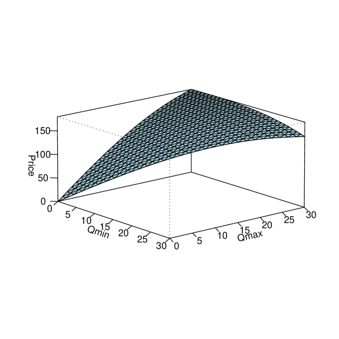
Figure 4: The mapping $Q\mapsto\widehat{P}^{n}_{0}(Q)$ affinely interpolated from integral-valued global constraints.

Acknowledgement: We thank Anne-Laure Bronstein for helpful comments.

References

• [1] Bally V., Pagès G., Printems J. (2001). A stochastic quantization method for non-linear problems, Monte Carlo Methods and Applications, 7, n01-2, pp.21-34.
• [2] Bally V., Pagès G. (2001). A quantization algorithm for solving multi-dimensional optimal stopping problems, Bernoulli, 6(9), 1-47.
• [3] Bally V., Pagès G. (2003). Error analysis of the quantization algorithm for obstacle problems, Stochastic Processes & Their Applications, 106(1), 1-40.
• [4] Bally V., Pagès G., Printems J. (2005). A quantization tree method for pricing and hedging multi-dimensional American options, Mathematical Finance, 15(1), 119-168.
• [5] Bardou O., Bouthemy S., Pagès G. (2006) Pricing swing options using Optimal Quantization.
• [6] Barrera-Esteve C., Bergeret F., Dossal C., Gobet E., Meziou A., Munos R., Reboul-Salze D. (2006) Numerical methods for the pricing of swing options: a stochastic control approach, Methodology and Computing in Applied Probability.
• [7] Carmona R. and Ludkovski M. (2007) Optimal Switching with Applications to Energy Tolling Agreements, pre-print.
• [8] Carmona R. and Ludkovski M. (2005) Gas Storage and Supply Guarantees : An Optimal Switching Approach, pre-print.
• [9] Carmona R. and Dayanik S. (2003) Optimal Multiple-Stopping of Linear Diffusions and Swing Options, pre-print.
• [10] Carmona R. and Touzi N. (2004) Optimal multiple stopping and valuation of swing options, Mathematical Finance, to appear.
• [11] Clewlow L., Strickland C. and Kaminski V. (2002) Risk Analysis of Swing Contracts, Energy and power risk management.
• [12] Geman H. (2005) Commodities and commodity derivatives - Modeling and Pricing for Agriculturals, Metals and Energy, Wiley Finance.
• [13] Gersho A., Gray R.M., Special issue on Quantization, IEEE Trans. on Inf. Theory, 29, $n^{0}1$&$2$, 1982.
• [14] Gersho A., Gray R.M. (1992). Vector Quantization and Signal Compression, Kluwer, Boston.
• [15] Graf S., Luschgy H., Foundations of Quantization for Probability Distributions. Lect. Notes in Math. 1730, Springer, Berlin.
• [16] Graf S., Luschgy H., Pagès, G., Distortion mismatch in the quantization of probability measures, to appear in ESAIM P& S, prep-print LPMA-$1051$.
• [17] Jaillet P., Ronn E.I., Tompaidis (2004). Valuation of Commodity-Based Swing Options, Management Science, 50, 909-921.
• [18] Keppo J. (2004) Pricing of Electricity Swing Options, Journal of Derivatives, 11, 26-43.
• [19] Lari-Lavassani A., Simchi M., Ware A. (2001) A discrete valuation of Swing options, Canadian Applied Mathematics Quarterly, 9(1), 35-74.
• [20] F. Longstaff and E.S. Schwartz (2001) Valuing American Options by Simulation: A Simple Least Squares Approach, The Review of Financial Studies, 14, 113-147.
• [21] Luschgy H., Pagès G., (2006). Functional quantization rate and mean regularity of processes with an application to Lévy processes, pre-pub. LPMA-1048.
• [22] Meinshausen N. and Hambly B.M. (2004) Monte Carlo methods for the valuation of multiple exercise options, Mathematical Finance , 14, $n^{0}4$.
• [23] Pagès G. (1998) A space vector quantization method for numerical integration, J. Computational and Applied Mathematics, 89, 1-38.
• [24] Pagès G., Pham H., Printems J. (2004). An Optimal Markovian Quantization Algorithm for Multidimensional Stochastic Control Problems, Stochastics and Dynamics, 4, 501-545.
• [25] Pagès G., Pham H., Printems J. (2004). Optimal quantization methods and applications to numerical problems in finance, Handbook of Numerical Methods in Finance, ed. S. Rachev, Birkhauser, 253-298.
• [26] Pagès G., Printems J. (2003). Optimal quadratic quantization for numerics: the Gaussian case, Monte Carlo Methods and Applications, 9, n${}^{0}2$, pp.135-166.
• [27] Ross S.M. and Zhu Z. (2006) Structure of swing contract value and optimal strategy, The 2006 Stochastic Modeling Symposium and Investment Seminar, Canadian Institute of Actuaries
• [28] Thompson A.C. (1995) Valuation of path-dependent contingent claims with multiple exercise decisions over time: the case of Take or Pay. Journal of Financial and Quantitative Analysis, 30, 271-293.
• [29] Winter C. and Wilhelm M. (2006) Finite Element Valuation of Swing Options, pre-print.
• [30] Zador P.L. (1982). Asymptotic quantization error of continuous signals and the quantization dimension, IEEE Trans. Inform. Theory, 28, Special issue on quantization, A. Gersho & R.M. Grey eds, 139-149.