Birefringence and non-transversality of light propagation in an ultra-strongly magnetized vacuum

Abstract

The birefringence phenomenon in the vacuum with a constant magnetic background of arbitrary strength is considered within the framework of the effective action approach. A new feature of the birefringence in a magnetized vacuum is that the parallel mode, which is polarized parallel to the plane containing the magnetic field and the photon wave vector, is no longer transverse. We have studied this feature in detail for arbitrary magnetic field and provided analytic results for the ultra-strong magnetic field regime. Possible physical implications of our results in astrophysics are discussed.

I Introduction

The theoretical investigation of nonlinear effects on light propagation, including vacuum birefringence, has been extensively studied since early 70s birula ; brezin ; adler ; shabad . Recent years have witnessed a significant growth of interest in this realm of research daniels ; dittgies ; dittbook ; salim ; pak ; heinzl , especially in the vacuum birefringence in ultra-strong fields, due to predictions of presence of strong magnetic fields in astrophysical objects pulsar ; astro ; shaviv and the technological improvement in high-intensity laser fields laser above the critical strength $B_{c}={\displaystyle{m^{2}c^{2}\over e\hbar}}\simeq 4.4\times 10^{13}G$. The birefringence phenomenon in magnetized media reveals a new interesting feature related with the fact that the polarization vector of the parallel mode of the propagating photon becomes non-transverse, i.e., it fails to be orthogonal to the wave vector brezin ; dittbook . One way of investigating the vacuum birefringence is to work within the effective Lagrangian approach. Recently the analytic series representation for the one-loop effective action of quantum electrodynamics (QED) has been obtained qed1 on the base of Schwinger’s integral expression for the effective action schw . This explicit analytical expression is helpful to investigate the light propagation in magnetic field of arbitrary strength, especially in strong magnetic fields of magnitude $B$ above the critical value $B_{c}$.

In the present paper we consider the birefringence in arbitrary homogeneous magnetic field as well as the effect of light non-transversality between the polarization vector and the wave vector. Since this effect is small (it is of second order in the fine structure constant) it was neglected for the field $B$ satisfying $0\leq B\leq{\cal O}(B_{c})$ in previous studies brezin ; dittbook . For ultra-strong magnetic field regime, $B>>B_{c}$, one should expect this effect will affect the propagation of light significantly. The purpose of our paper is to investigate this effect in a detail for magnetic field of arbitrary strength.

II Effective action formalism

The effective action provides us with a useful bridge between the full quantum theory and classical field theory. Once the effective action is known, in soft photon approximation (photon energy smaller than the electron mass), classical equations of motion can be derived to describe the light propagation in the language of classical physics.

Let us start with the main lines of the effective action approach to light propagation in various vacua dittgies ; visser . An integral expression for the one-loop effective action is given by Schwinger schw

$${\cal L}_{\mathrm{eff}} = -x-{\displaystyle{1\over 8\pi^{2}}}\int_{0}^{\infty}{\displaystyle{dt\over t^{3}}}e^{-m^{2}t}\Bigg{[}-{\displaystyle{2\over 3}}(et)^{2}x-1$$ (1)

$$+(et)^{2}|y|\coth\Bigg{(}et\sqrt{\sqrt{x^{2}+y^{2}}+x}\Bigg{)}\cot\Bigg{(}et\sqrt{\sqrt{x^{2}+y^{2}}-x}\Bigg{)}\Bigg{]},$$

where we have introduced the gauge and Lorentz invariants of the electromagnetic field,

$$x={\displaystyle{1\over 4}}F_{\mu\nu}F^{\mu\nu},$$

$$y={\displaystyle{1\over 4}}F_{\mu\nu}{\tilde{F}}^{\mu\nu},~{}~{}{\tilde{F}}^{\mu\nu}={\displaystyle{1\over 2}}\epsilon^{\mu\nu\rho\sigma}F_{\rho\sigma}.$$ (2)

We employ $\epsilon^{0123}=-1$ and $\eta_{\mu\nu}=\mathrm{diag}(-1,1,1,1)$. We use Greek letters for the space-time indices $(0,1,2,3)$ and Latin letters for the spatial ones. For convenience, we use natural units $\hbar=c=1$ throughout the paper.

To obtain exact analytic results we will use an exact series representation for the one-loop effective Lagrangian of QED qed1

$${\cal L} = -{\displaystyle{a^{2}-b^{2}\over 2}}$$ (3)

$$-{\displaystyle{e^{2}\over 4\pi^{3}}}ab\sum_{n=1}^{\infty}{\displaystyle{1\over n}}\Big{[}\coth({\displaystyle{n\pi b\over a}})\Big{(}{\rm ci}({\displaystyle{n\pi m^{2}\over ea}})\cos({\displaystyle{n\pi m^{2}\over ea}})+{\rm si}({\displaystyle{n\pi m^{2}\over ea}})\sin({\displaystyle{n\pi m^{2}\over ea}})\Big{)}$$

$$-{\displaystyle{1\over 2}}\coth({\displaystyle{n\pi a\over b}})\Big{(}\exp({\displaystyle{n\pi m^{2}\over eb}}){\rm Ei}(-{\displaystyle{n\pi m^{2}\over eb}})+\exp(-{\displaystyle{n\pi m^{2}\over eb}}){\rm Ei}({\displaystyle{n\pi m^{2}\over eb}})\Big{)}\Big{]},$$

where $a,b$ are gauge invariant variables corresponding to the magnetic and electric fields in an appropriate Lorentz frame,

$$a=\sqrt{\sqrt{x^{2}+y^{2}}+x},$$

$$b=\sqrt{\sqrt{x^{2}+y^{2}}-x}.$$ (4)

In the weak field limit the expansion of the integral in (1) produces the well-known Euler-Heisenberg effective Lagrangian ritus ; dittgies

$$\tilde{\cal L}_{\mathrm{E-H}}=-x+\tilde{c}_{1}x^{2}+\tilde{c}_{2}y^{2},$$

$$\tilde{c}_{1}={\displaystyle{8\alpha^{2}\over 45m^{4}}},~{}~{}~{}~{}\tilde{c}_{2}={\displaystyle{14\alpha^{2}\over 45m^{4}}},$$ (5)

where $\alpha={\displaystyle{e^{2}\over 4\pi\epsilon_{0}}}={\displaystyle{1\over 137.036}}$ is the fine structure constant. In our choice of natural units we set $\epsilon_{0}=1$, so that the corresponding value of electron charge is $e=\sqrt{4\pi\alpha}$.

We will follow the effective action approach visser to study the light propagation effects in nonlinear electrodynamics. We assume that the soft photon approximation, the linearization procedure, and the restricted eikonal approximation make sense visser . It is suitable to split the total electromagnetic field into the background field $F_{\mu\nu}$ and the propagating photon $f_{\mu\nu}$ with the vector potential $a_{\mu}(k)$ and wave vector $k^{\mu}$. We keep the linear approximation with respect to $f_{\mu\nu}$ in equations of motion. After these two procedures the equations of motion corresponding to the full effective action lead to an eigenvalue equation for the propagating modes,

$$A^{\mu\nu}\epsilon_{\nu}=0,$$ (6)

where $\epsilon_{\nu}\equiv a_{\nu}/(a_{\mu}a^{\mu})^{1/2}$ is a unit polarization vector of the soft photon, the symmetric tensor $A^{\mu\nu}$ is given by

$$A^{\mu\nu} \equiv 2\left.{{\partial^{2}{\cal L}\over\partial F_{\mu\alpha}\;\partial F_{\nu\beta}}}\right|_{\mathrm{background}}k_{\alpha}k_{\beta}$$ (7)

$$= c_{1}F^{\mu\alpha}F^{\nu\beta}k_{\alpha}k_{\beta}+c_{2}\tilde{F}^{\mu\alpha}\tilde{F}^{\nu\beta}k_{\alpha}k_{\beta}+c_{3}(\delta^{\mu\nu}k^{2}-k^{\mu}k^{\nu})$$

$$+c_{5}(F^{\mu\alpha}\tilde{F}^{\nu\beta}+\tilde{F}^{\mu\alpha}F^{\nu\beta})k_{\alpha}k_{\beta},$$

and the derivative functions are defined by

$$c_{1}\equiv\frac{1}{2}\partial_{x}^{2}{\cal L},~{}~{}c_{2}\equiv\frac{1}{2}\partial_{y}^{2}{\cal L},~{}~{}c_{3}\equiv\frac{1}{2}\partial_{x}{\cal L},~{}~{}c_{4}\equiv\frac{1}{2}\partial_{y}{\cal L},~{}~{}c_{5}\equiv\frac{1}{2}\partial_{xy}{\cal L}.$$ (8)

It can be shown salim that the equation (6) is indeed equivalent to the light cone condition obtained in dittgies without using the averaging over polarization modes.

Solutions of equation (6) represent the dynamically allowed polarization modes. Nontrivial solutions to this equation exist if a generalized Fresnel equation is satisfied kremer

$$\det A^{\mu\nu}(k)=0.$$ (9)

In fact, it is a scalar equation for $k$ and thus implicitly represents the dispersion relation for the light propagation in the polarized QED vacuum. A suitable choice of gauge fixing for $a_{\mu}$ simplifies the eigenvalue problem (6). We will use a physical temporal gauge $a_{0}=\epsilon_{0}=0$, since it directly links the polarization vector $\vec{\epsilon}$ to the electric field of the propagating photon $\vec{e}$, $\vec{\epsilon}=\vec{e}/|\vec{e}|$. With this gauge the eigenvalue equation (6) splits into the equation

$$A^{0i}\,\epsilon_{i}=0,$$ (10)

and the reduced eigenvalue problem

$$A^{ij}\,\epsilon_{j}=0\,.$$ (11)

The latter implies the following condition

$$\mbox{det}\left(A^{ij}\right)=0.$$ (12)

There are two independent physical modes of the eigenvalue problem (11), so that the space of polarizations is at most two-dimensional birula ; visser .

III vacuum birefringence in Magnetic Field

In this section we first obtain the general equations for the light velocity and polarization vector. Then we apply these equations to both the truncated one-loop effective Euler-Heisenberg Lagrangian, Eq. (5), and the series representation for the one-loop effective Lagrangian, Eq. (3), in both the weak and strong magnetic field regions. For the case of ultra strong magnetic field we derive asymptotic formulae as well.

Without loss of generality, we choose the magnetic field directed along the $z$-axis, $\vec{B}=(0,0,a)$. We assume the wave vector $\vec{k}$ lies in the plane $xOz$, so that $\bar{k}^{\mu}=k^{\mu}/|{\vec{k}}|=(v,\sin\theta,0,\cos\theta)$ (Fig. 1), and we will not distinguish between ${\bar{k}}$ and $k$ below. Hereafter the coefficient functions $c_{i}$ in (8) are taken in the limit of vanishing electric field, $b\rightarrow 0$ ($y\rightarrow 0$). Since in standard QED the effective Lagrangian ${\cal L}_{\mathrm{eff}}$ is an even function of $y$ we find

$$c_{4}=0,~{}~{}~{}~{}c_{5}=0.$$ (13)

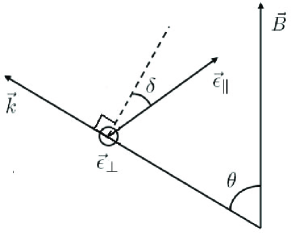
Figure 1: Two modes of light propagation in a magnetized vacuum. $\delta=\angle(\vec{\epsilon}_{\parallel},\vec{k})-{\displaystyle{\pi\over 2}}$. $\vec{\epsilon}_{\bot}$ is orthogonal to the plane containing $\vec{B}$ and $\vec{k}$.

The explicit solution to the eigenvalue equation (11) provides two independent polarization vectors, $\vec{\epsilon}_{\bot}$ and $\vec{\epsilon}_{\parallel}$, corresponding to the orthogonal and parallel modes respectively

$$\vec{\epsilon}_{\bot} = (0,~{}1,~{}0),$$

$$v^{2}_{\bot} = 1+\frac{c_{1}a^{2}\sin^{2}\theta}{c_{3}},$$

$$\vec{\epsilon}_{\parallel} = {\displaystyle{1\over\rho(\theta)}}\big{(}(c_{3}-a^{2}c_{2})\cos\theta,~{}0,~{}-c_{3}\sin\theta\big{)},$$

$$v^{2}_{\parallel} = 1-\frac{c_{2}a^{2}\sin^{2}\theta}{c_{2}a^{2}-c_{3}},$$ (14)

where $\rho(\theta)=\sqrt{c_{3}^{2}+a^{2}c_{2}(a^{2}c_{2}-2c_{3})\cos^{2}\theta}$ is the normalization factor. One can check that the solution is consistent with Eq. (10). It is worthwhile to notice that the polarization vector $\vec{\epsilon}_{\parallel}$ is not orthogonal to the wave vector $\vec{k}$. The deviation angle defined by $\delta=\angle(\vec{\epsilon}_{\parallel},\vec{k})-{\displaystyle{\pi\over 2}}$ takes the form

$$\cot\delta=\cot\theta-\frac{2c_{3}}{a^{2}c_{2}\sin 2\theta}.$$ (15)

The existence of $\delta$ is analogous to the light propagation in crystal optics, in which the non-orthogonality between the photon electric field and wave vector often occurs. In some sense, the vacuum in magnetic field behaves as a ”uniaxial crystal”.

Now we can apply the above formal equations to the one-loop effective Euler-Heisenberg Lagrangian, Eq. (5). Simple calculation leads to the following results

$$v^{2}_{\bot} = 1-\frac{2a^{2}\tilde{c}_{1}\sin^{2}\theta}{1-a^{2}\tilde{c}_{1}},$$

$$v^{2}_{\parallel} = 1-\frac{2a^{2}\tilde{c}_{2}\sin^{2}\theta}{1-a^{2}(\tilde{c}_{1}-2\tilde{c}_{2})},$$

$$\cot\delta = \cot\theta+\frac{1-a^{2}\tilde{c}_{1}}{a^{2}\tilde{c}_{2}\sin 2\theta}.$$ (16)

We apply the above formal equations to exact one-loop effective Lagrangian, Eq. (3). One can calculate the coefficient functions $c_{i}$ in terms of the main function $G(a)$ pak

$$c_{1} = {\displaystyle{1\over 2a^{3}}}(a\partial^{2}_{a}{\cal L}-\partial_{a}{\cal L}),$$

$$c_{2} = {\displaystyle{1\over 2a^{3}}}(a\partial^{2}_{b}{\cal L}+\partial_{a}{\cal L}),$$

$$c_{3} = {\displaystyle{1\over 2a}}\partial_{a}{\cal L},$$

$$c_{4} = {\displaystyle{1\over 2a}}\partial_{b}{\cal L},$$

$$\partial_{a}{\cal L} = -a-{\displaystyle{e^{2}a\over 2\pi^{4}}}G(a)-{\displaystyle{e^{2}a^{2}\over 4\pi^{4}}}G^{\prime}(a),$$

$$\partial_{b}{\cal L} = 0,$$

$$\partial^{2}_{a}{\cal L} = -1-{\displaystyle{e^{2}\over 2\pi^{4}}}G(a)-{\displaystyle{e^{2}a\over\pi^{4}}}G^{\prime}(a)-{\displaystyle{e^{2}a^{2}\over 4\pi^{4}}}G^{\prime\prime}(a),$$

$$\partial^{2}_{b}{\cal L} = 1+{\displaystyle{e^{4}a^{2}\over 36\pi^{2}m^{4}}}+{\displaystyle{e^{4}a^{3}\over 3\pi^{4}m^{4}}}G^{\prime}(a)+{\displaystyle{e^{4}a^{4}\over 6\pi^{4}m^{4}}}G^{\prime\prime}(a),$$ (17)

where

$$G(a) = \sum_{n=1}^{\infty}{\displaystyle{1\over n^{2}}}g({\displaystyle{n\pi m^{2}\over ea}}),$$

$$g(x) = {\rm ci}(x)\cos x+{\rm si}(x)\sin x.$$ (18)

The function $G(a)$ determines the one-loop contribution to the effective Lagrangian with a pure magnetic background pak , and it can be written in terms of the generalized Hurvitz $\zeta$-function as well.

With the Eqs. (14) and (17), the light velocities and the angle $\delta$ can be expressed as follows

$$v^{2}_{\bot} = 1+{\displaystyle{{\displaystyle{e^{2}a\over 4\pi^{4}}}\sin^{2}\theta(3G^{\prime}(a)+aG^{\prime\prime}(a))\over 1+{\displaystyle{e^{2}\over 4\pi^{4}}}(2G(a)+aG^{\prime}(a))}},$$

$$v^{2}_{\parallel} = {\Big{(}}1+{\displaystyle{e^{4}a^{2}\cos^{2}\theta\over 36\pi^{2}m^{4}}}+{\displaystyle{e^{2}\sin^{2}\theta\over 2\pi^{4}}}G(a)$$

$$+({\displaystyle{e^{4}a^{3}\cos^{2}\theta\over 3\pi^{4}m^{4}}}+{\displaystyle{e^{2}a\sin^{2}\theta\over 4\pi^{4}}})G^{\prime}(a)+{\displaystyle{e^{4}a^{4}\over 6m^{4}\pi^{4}}}\cos^{2}\theta G^{\prime\prime}(a){\Big{)}}$$

$$\cdot{\Big{(}}1+{\displaystyle{e^{4}a^{2}\over 36\pi^{2}m^{4}}}+{\displaystyle{e^{4}a^{3}\over 3\pi^{4}m^{4}}}G^{\prime}(a)+{\displaystyle{e^{4}a^{4}\over 6m^{4}\pi^{4}}}G^{\prime\prime}(a){\Big{)}}^{-1},$$

$$\cot\delta = \cot\theta+{\displaystyle{\csc\theta\sec\theta{\Big{(}}1+{\displaystyle{e^{2}\over 2\pi^{4}}}G(a)+{\displaystyle{e^{2}a\over 4\pi^{4}}}G^{\prime}(a){\Big{)}}\over{\displaystyle{e^{4}a^{2}\over 36\pi^{2}m^{4}}}-{\displaystyle{e^{2}\over 2\pi^{4}}}G(a)+({\displaystyle{e^{4}a^{3}\over 3\pi^{4}m^{4}}}-{\displaystyle{e^{2}a\over 4\pi^{4}}})G^{\prime}(a)+{\displaystyle{e^{4}a^{4}\over 6m^{4}\pi^{4}}}G^{\prime\prime}(a)}}.$$ (19)

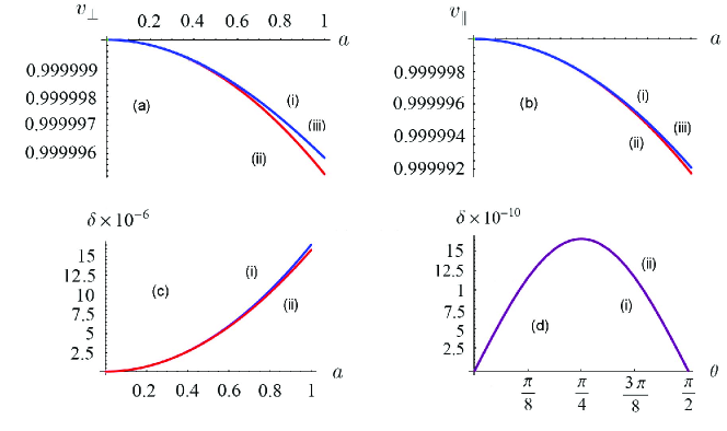
Figure 2: Light propagation in weak magnetic field, $\vec{B}=(0,0,a)$. (a) Light velocity of $\bot$ mode; (b) light velocity of $\parallel$ mode; (c) the dependence of $\delta$ on the field strength $\tilde{a}$ at $\theta={\displaystyle{\pi\over 4}}$; (d) the dependence of $\delta$ on $\theta$ at $\tilde{a}=0.01$ (the two curves are quite adjacent). (i) an exact one-loop approximated result; (ii) the result in weak field approximation; (iii) the result obtained in Ref. pak . The dimensionless magnetic field strength $\tilde{a}={\displaystyle{a\over m^{2}}}$ is measured in units of electron mass, the critical value is $\tilde{a}_{c}={\displaystyle{1\over e}}\simeq 3.3$. The magnetic field strength $B$ in standard units is given by $B={\tilde{a}}\times\sqrt{4\pi\alpha}B_{c}$.

In order to confirm our results, we compare them with the results obtained in the past for the particular case of vacuum birefringence in weak field limit. For $\theta={\displaystyle{\pi\over 4}}$ the light velocities for ($\bot,\parallel$)-modes are plotted in Fig. (2a) and (2b). The dependence of $\delta$ on the field strength $a$ and on $\theta$ is shown in Fig. (2c) and (2d) respectively.

For the case of weak field regime, the $\delta$ angle is quite small as expected, $\delta\simeq a^{2}\tilde{c}_{2}\sin 2\theta$. For moderate magnetic fields satisfying the condition $-{\displaystyle{c_{3}\over c_{2}a^{2}}}\gg 1$ we have a simple relation

$$\delta\simeq-{\displaystyle{c_{2}a^{2}\over 2c_{3}}}\sin 2\theta.$$ (20)

Now, let us consider light velocity in the strong field region. From the asymptotic behaviour of the function $G(a)$ pak

$$G(a) = -{\displaystyle{\pi^{2}\over 6}}(\ln{\displaystyle{ea\over m^{2}}}+d_{1})-{\displaystyle{\pi^{2}m^{2}\over 2ea}}(\ln{\displaystyle{ea\over\pi m^{2}}}+1)-{\displaystyle{\pi^{2}m^{4}\over 4e^{2}a^{2}}}(\ln{\displaystyle{2ea\over\pi m^{2}}}-\gamma+{\displaystyle{5\over 2}}),$$

$$d_{1} = -\gamma-\ln\pi+{\displaystyle{6\over\pi^{2}}}\zeta^{\prime}(2)=-2.29191...~{},$$ (21)

one can derive the following asymptotic equations for the light velocities $v_{\bot,\parallel}$ and angle $\delta$ in an ultra-strong magnetic field

$$v^{2}_{\bot} \simeq {\displaystyle{1-{\displaystyle{e^{2}\over 12\pi^{2}}}(\ln{\displaystyle{ea\over m^{2}}}+d_{1}+{\displaystyle{1\over 2}}+\sin^{2}\theta)\over 1-{\displaystyle{e^{2}\over 12\pi^{2}}}(\ln{\displaystyle{ea\over m^{2}}}+d_{1}+{\displaystyle{1\over 2}})}}\,$$

$$= 1+{\cal O}(B_{c}/a),$$

$$v^{2}_{\parallel} \simeq {\displaystyle{1-{\displaystyle{e^{2}\over 12\pi^{2}}}(\ln{\displaystyle{ea\over m^{2}}}+d_{1}-d_{2}\cos^{2}\theta+{\displaystyle{1\over 2}})+{\displaystyle{ae^{3}\over 12\pi^{2}m^{2}}}\cos^{2}\theta\over 1-{\displaystyle{e^{2}\over 12\pi^{2}}}(\ln{\displaystyle{ea\over m^{2}}}+d_{1}-d_{2}+{\displaystyle{1\over 2}})+{\displaystyle{e^{3}a\over 12\pi^{2}m^{2}}}}}\,$$

$$= \cos^{2}\theta+{\cal O}(B_{c}/a),$$

$$\cot\delta \simeq \cot\theta-{\displaystyle{2\ln{\displaystyle{ae\over m^{2}}}+1+2d_{1}-{\displaystyle{24\pi^{2}\over e^{2}}}\over\sin 2\theta({\displaystyle{ae\over m^{2}}}+d_{2})}}\,$$

$$= \cot\theta-{\displaystyle{1\over\sin 2\theta}}{\cal O}(B_{c}/a),$$

$$d_{2} = d_{1}-{\displaystyle{1\over 2}}+\gamma+\ln{\displaystyle{\pi\over 2}}=-1.76311...~{}.$$ (22)

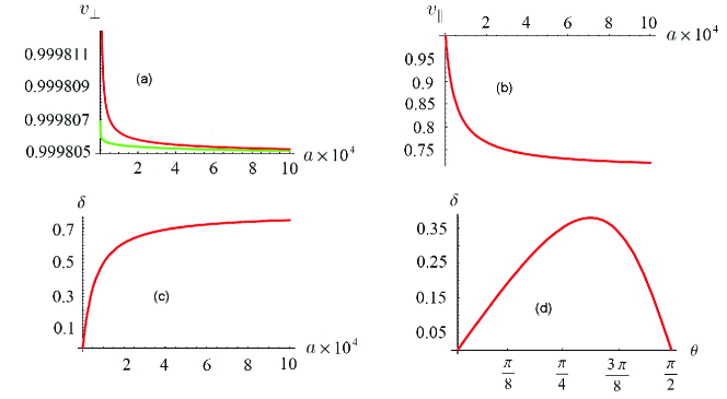
Figure 3: Light propagation in strong magnetic field. (a) Light velocity of $\bot$ mode, the upper is exact one-loop approximated result while the lower is asymptotic result; (b) light velocity of $\parallel$ mode; (c) the dependence of $\delta$ on the field strength $\tilde{a}$ at $\theta={\displaystyle{\pi\over 4}}$; (d) the dependence of $\delta$ on $\theta$ at $\tilde{a}=5\times 10^{3}$. (In (b), (c) and (d) the two curves of exact result and asymptotic result are quite adjacent). The dimensionless magnetic field strength $\tilde{a}={\displaystyle{a\over m^{2}}}$ is measured in units of electron mass.The maximal terms of numerically calculating $G(a)$ is $2\times 10^{4}$ for the maximal field.

Comparing these asymptotic formulae with the results obtained in pak , one can conclude that the velocities of orthogonal mode coincide while the velocities of parallel mode differ essentially in the asymptotic limit. The deviation angle $\delta$ can be quite large within $[0,{\displaystyle{\pi\over 2}})$. When $\theta$ approaches the value ${\displaystyle{\pi\over 2}}$ the angle $\delta$ vanishes, i.e., the light becomes transverse.

It is well known that the strength of an electric field is limited by the ”Klein Catastrophe” while the strength of a magnetic field is not. But there are several other physical limits that apply to magnetic fields zaumen ; lerche . For example, diverse interactions with photons and matter deplete energy and momentum from the neutron star field, limiting its strength to $B_{max}<10^{16}-10^{18}G$ lerche . This typical value of order $10^{18}G$ determines the range of strength of considered magnetic field.

In Fig. (3a) and (3b) the light velocities $v_{\bot,\parallel}$) at $\theta={\displaystyle{\pi\over 4}}$ are presented in the strong field regime. The dependence of $\delta$ on the field strength $a$ and on the $\theta$ is shown in Fig. (3c) and (3d) respectively.

The results are still reasonable even in the asymptotic limit since the phase velocities keep bounded, $0\leq v_{\bot,\parallel}\leq 1$. In fact, the orthogonal mode propagates as in the trivial vacuum, independent of the wave vector. On the other hand, the phase velocity of the parallel mode is directly associated to the direction of propagation. The propagation perpendicular to the magnetic field ($v_{\parallel}(\theta={\displaystyle{\pi\over 2}})=0$) is strictly forbidden, while the parallel propagation is preferred $\big{(}v_{\parallel}(\theta=0)=1\big{)}$, in agreement with the previous results dittbook . As a result, photons in the $\parallel$ mode eventually propagate along the magnetic field, regardless of their incidence angle $\theta$. So that, since $\delta=\theta$ for $\theta\in[0,{\displaystyle{\pi\over 2}})$ in the asymptotic limit, the polarization vector of the $\parallel$ mode is mostly directed along the $x$ axis (except for $\theta={\displaystyle{\pi\over 2}}$), irrelevant to the wave vector.

Using the equations for the light the velocities (14), one can derive the corresponding refraction indices

$$n^{2}_{\bot,\parallel}={\displaystyle{1\over v^{2}_{\bot,\parallel}}}.$$ (23)

With Eq. (22) one can approximate the refraction index by

$$n_{\bot} \simeq 1,$$

$$n_{\parallel} \simeq \big{(}{{\displaystyle{1+{\displaystyle{e^{3}a\over 12\pi^{2}m^{2}}}\over 1+{\displaystyle{e^{3}a\over 12\pi^{2}m^{2}}}\cos^{2}\theta}}}\big{)}^{\frac{1}{2}},$$ (24)

in agreement with results obtained before shabad ; shabadnew .

Our results can be helpful in study of the light propagation in a pure electric field background or crossed field background ($\vec{E}\bot\vec{B}$, $|\vec{E}|=|\vec{B}|$). For these two cases it is readily verified that $y=0$ still holds and thus $c_{4}=c_{5}=0$. So the calculation is straightforward by analogy with the above results. For example, in a pure electric field, interchanging of $c_{1}$ and $c_{2}$ in (14) will give the desired results.

IV Conclusion

We have analyzed the light propagation in a constant magnetic field of arbitrary strength. Within effective action approach we have investigated the features of the propagation modes in both the weak and strong field regimes. We have demonstrated that the polarization vector of the parallel mode is no longer orthogonal to the wave vector. The effect of non-transversality is enhanced in strong field regime and significantly affects the asymptotic behavior of light velocity. The analytic asymptotic formulae of light velocities and deviation angle $\delta$ for strong magnetic field have been obtained.

We would like to discuss two potential applications of our results in astrophysics. The first one is related to magnetic lensing effect which appears when the fields are significantly stronger than $B_{c}$ (see, e.g., shaviv ). For example, for at least five known gamma-pulsars the magnetic field exceeds $B_{c}$, and for magnetars the magnitude of magnetic field is estimated to be of order $10^{14}-10^{15}$G pulsar . The main result of the lensing effect is that the effective surface areas of the astrophysical object measured by two polarization states are different. Since the parallel mode is no longer transverse, the measurement of its polarization responses accordingly. Especially, the dependence of the deviation angle $\delta$ on the incidence angle $\theta$ should be important in the determination of the effective surface area of polarizations. This consequence in the measurement will be strengthened in the strong magnetic field. From the numerical results in Fig. 2, one may argue that the new feature of non-transversality is negligible at $B\sim B_{c}$ compared to traditional approach; however, for astronomical distances, even a very small deviation can lead to essentially different observations. Another possible application might be related to the effect of strongly enhanced mode coupling in light scattering (see, e.g., bulik ; ozel ). When photons propagate through scattering in the magnetized plasma they can change their polarization modes as well as their directions and energy. This effect can change the total spectrum and angular distribution of radiation from the neutron star. When the photons interact with both the electrons and the protons in the plasma, a careful analysis of photon polarization effects is necessary for precise calculation. We hope that our results can provide a better quantitative description of these effects and possibly other astrophysical phenomena related to birefringence in ultra-strong magnetic fields.

Acknowledgments The authors would like to thank Prof. D. G. Pak for suggesting this work. We also thank Prof. Mo-Lin Ge and Prof. Yi Liao for their encouragement and helpful discussions.

References

• (1) Brezin E and Itzykson C 1971 Phys. Rev. D 3 618
• (2) Batalin I A and Shabad A E 971 ZhETF 1 60 894 (1971 Sov. Phys. - JETP 33 483 )
• (3) Adler S L 1971 Ann. Phys. 67 599 Tsai W Y and Erber T 1975 Phys. Rev. D 12 1132 Tsai W Y 1974 Phys. Rev. D 10 2699 Baier V N, Katkov V M and Strakhovenko 1975 ZhETF 68 403 Drummond I T and Hathrell S J 1980 Phys. Rev. D 22 343
• (4) Bialynicka-Birula Z and Bialynucki-Birula I 1970 Phys. Rev. D 2 2341
• (5) Daniels R D and Shore G M 1994 Nuclear Phys. B 425 634 Latorre J I, Pascual P and Tarrach R 1995 Nuclear Phys. B 437 60 Shore G M 1996 Nuclear Phys. B 460 379
• (6) Dittrich W and Gies H 1998 Phys. Rev. D 58 025004 Dittrich W and Gies H 1998 Phys. Lett. B 431 420 Dittrich W and Gies H 1998 Vacuum Birefringence in Strong Magnetic Fields, Proc. of Frontier Tests of Quantum Electrodynamics and Physics of the Vacuum, Sandansky 1998( 1998 Heron Press 29) (Preprint hep-ph/9806417).
• (7) Dittrich W and Gies H 2000 Probing The Quantum Vacuum (Springer Tracts in Modern Physics. Vol 166) (Springer)
• (8) De Lorenci V A, Klippert R, Novello M and Salim J M 2000 Phys.Lett. B 482 134
• (9) Cho Y M, Pak D G and Walker M L 2006 Phys.Rev. D 73 065014
• (10) Itin Y 2005 Phys. Rev. D 72 087502 Heinzl T et al 2006 Opt. Commun. 267 318 Heinzl T and Schroeder O 2006 J.Phys. A 39 11623 Adler S. L 2007 J. Phys. A 40 F143 Biswas S and Kirill Melnikov 2007 Phys.Rev. D 75 053003
• (11) Shaviv N J, Heyl J S and Lithwick Y 1999 MNRAS 306 333
• (12) Kaspi V M 1999 Pulsar Astronomy - 2000 and Beyond. ASP Conference Series 202 (Kramer M, Wex N and Wielebinski R eds.) astro-ph/9912284.
• (13) Duncan R C 2000 Preprint astro-ph/0002442 van Putten M H P M 2000 Phys. Rev. Lett. 84 3752 and references therein
• (14) Burke D L et al 1997 Phys.Rev. Lett. 79 1626 Alkofer R, Hecht M B, Roberts C D, Schmidt S M and Vinnik D V 2001 Phys.Rev. Lett. 87 193902 Roberts C D, Schmidt S M and Vinnik D V 2002 Phys.Rev. Lett. 89 153901 Shen B and Yu M Y 2002 Phys.Rev. Lett. 89 275004; for review and references, see Ringwald A 2003 Preprint hep-ph/0304139
• (15) Cho Y M and Pak D G 2001 Phys. Rev. Lett. 86 1947 Mielniczuk W 1982 J. Phys. A 15 2905
• (16) Schwinger J 1951 Phys. Rev. 82 664
• (17) Liberati S, Sonego S and Visser M 2001 Phys. Rev. D 63 0850013
• (18) Ritus V 1976 JETP 42 774 Ritus V 1977 JETP 46 423 Reuter M Schmidt M and Schubert C 1997 Ann. Phys, 259 313
• (19) Kremer H F 1965 Phys. Rev. 139 B254
• (20) Zaumen W T 1976 ApJ 210, 776 Zaumen W T 2003 Preprint astro-ph/0304120
• (21) Lerche I and Shramm D N 1977 ApJ 216 881
• (22) Shabad A E 2003 Preprint hep-th/0307214
• (23) Bulik T and Miller M C 1997 MNRAS 288 596
• (24) Ozel F 2003 Astrophys. J. 583 402