Higgs and Top quark coupled with a conformal gauge sector

Abstract

We propose a dynamical scenario beyond the standard model, in which the radiative correction to the Higgs mass parameter is suppressed due to a large anomalous dimension induced through a conformal invariant coupling with an extra gauge sector. Then the anomalous dimension also suppresses the Yukawa couplings of the Higgs field. However, the large top Yukawa coupling can be generated effectively through mixing among top quarks and the fermions of the conformal gauge sector. This scenario is found to predict a fairly heavy Higgs mass of about 500 GeV. We present an explicit model and show consistency with the Electro-Weak precision measurements of the S and T parameters as well as the Z boson decay width.

I Introduction

Unnaturalness of the standard model (SM) indicates that at least the Higgs sector is modified with new interactions and particles above some energy scale $M$ not much higher than 1 TeV. Especially, if the Higgs mass is less than $200$GeV, which is expected from the Electro-Weak (EW) precision tests LEP , then the scale $M$ should be no more than $O(1)$TeV. The origin of fine-tuning is the quadratic divergence in the radiative corrections to the Higgs mass parameter. Therefore the new physics above the scale $M$ must remove the quadratic divergence. However absence of the quadratic divergence is not sufficient phenomenologically. The EW precision tests constrain some dimension 6 operators added effectively to the EW theory severely GW and the scale of the new physics is expected to be higher than $5\sim 10$TeV generically LEPparadox . The discrepancy between this scale and the scale $M$ for naturalness is called the LEP paradox or the little hierarchy problem. Thus the new physics should have specific properties in order to be consistent with the EW precision tests simultaneously.

The quadratic divergence can be eliminated by imposing global symmetries. The most postulated candidate would be supersymmetry, which predicts a fairly light Higgs mass. The little Higgs models littlehiggs also assume global symmetries to suppress the quadratic divergence to mass of the Higgs boson appearing as a pseudo Nambu-Goldstone boson. Then the Higgs mass is predicted to be light again, since the Higgs quartic coupling is also suppressed due to the global symmetries. It should be also mentioned that the supersymmetric extension does not remove the hierarchy problem completely. The rigid supersymmetry restricts the Higgs mass to be less than the Z-boson mass $M_{Z}$. Meanwhile, the Higgs mass has been constrained to be heavier than 115GeV by LEPII LEP . Therefore, the scale of the supersymmetry breaking parameters must be rather large and a sizeable radiative correction to the Higgs mass is induced. Consequently, fine-tuning of a few percent is required to realize the EW symmetry breaking of 250GeV. There have been no convincing scenarios overcoming this problem, although various models have been proposed so far lowsusy ; extradterm ; fathiggs ; supersoft ; superlittle ; KNT . So it would be worth while seeking for other possibilities as well.

Although the results of the EW precision tests are consistent with the SM with a light Higgs boson, the heavy Higgs boson is not always excluded. The recent analysis shows that a heavy Higgs mass of 400-600 GeV can be consistent heavyhiggs ; BHR , as long as there are extra contributions leading to $\Delta T=0.25\pm 0.1$ and a small $\Delta S$ LEP . Therefore the possibility to find a heavy Higgs at LHC is still open, though the constraint to the new physics is rather restrictive. For example, the Technicolor models, in which the composite Higgs boson is rather heavy, are known to suffer from too large corrections to the S-parameter PT ; strongEW . Even if the Higgs boson is not a composite particle, the Higgs mass as heavy as the triviality bound, which is about 600GeV, implies that a strong interaction is involved with the Higgs sector at the TeV scale. Then large oblique corrections are generated in general. Meanwhile, the degree of fine-tuning to the Higgs mass parameter is ameliorated for a heavy Higgs mass and the scale of new physics may be raised up somewhat KM ; BHR . However the improvement is not significant and new physics should appear at a few TeV CEH .

In this paper, we study a dynamical scenario to protect the Higgs mass parameter from the quadratic diverging corrections. Suppose that the Higgs field acquires a positive anomalous dimension, then the degree of divergence of the mass correction is reduced. Therefore, if the anomalous dimension is sufficiently large, then cutoff dependence of the mass correction may be drastically suppressed and the Higgs sector is relieved from the fine-tuning problem. Indeed it will be shown that such a large anomalous dimension can be realized by introducing a coupling of the Higgs with a strongly interacting conformal field theory (CFT).

Recently Luty and Okui LO has also discussed a Higgs model with a large anomalous dimension, the “conformal Technicolor”, and it’s AdS/CFT correspondence AdS/CFT . In their scenario, the Higgs boson is given as a fermion composite. In this paper, we consider a scenario in which the EW symmetry breaking (EWSB) is not dynamical and the Higgs boson behaves as a point particle even above the TeV scale. Therefore the strongly coupled sector does not induce a large correction to $S$-parameter. In this respect, our scenario is distinct from the models discussed in Ref. LO and let us call it “the conformal Higgs model” hereafter. Explicitly, the CFT is assumed to be a strongly coupled gauge theory with a appropriate number of vector-like fermions and the Higgs boson interacts through a large Yukawa coupling with some of these fermions. Then it is found that the Higgs mass given in this scenario is as heavy as 500GeV due to the strong interaction, although the cutoff dependence is suppressed by the anomalous dimension.

In order to make such a scenario viable phenomenologically, we need to think about the following problems. First, we note that the large anomalous dimension of the Higgs also suppresses the Yukawa couplings with quarks and leptons. Therefore it seems that this scenario is incompatible with the large top quark mass. It may be suggestive that many approaches towards the little hierarchy problem are faced with difficulty to explain the top quark mass simultaneously. In order to avoid this problem, we suppose that the origin of the prominently large top quark mass is different from the Yukawa coupling with the Higgs boson. More explicitly, we consider that the dynamics producing masses for the extra vector-like fermions also induces mixing between top quarks and the extra fermions KNT . Then the top Yukawa coupling can be generated through the large Yukawa coupling of the Higgs with the extra fermions effectively.

Another problem to be concerned is consistency with the EW precision tests. As is mentioned above, the heavy Higgs boson requires a suitable amount of extra contributions to the $T$-parameter. In the present model, the custodial symmetry is largely violated, since only top quark fields are assumed to mix with the CFT sector significantly. Therefore the loop corrections with the extra fermions contribute to the $T$-parameter. The size of the correction depends on the masses of these fermions, which gives also the decoupling scale of the CFT sector from the EW theory. We will show an explicit model with the decoupling scale of a few TeV can explain the $T$-parameter consistent with the EW precision test.

Recently various alternative EWSB scenarios defined in the warped extra dimensions, or the five-dimensional anti-de Sitter (AdS) space, with four-dimensional boundaries AdS/CFT have been studied extensively, e.g. the Higgsless models higgsless , the minimal composite Higgs models minimalcomposite . The studies of these models also revealed that it is a rather non-trivial problem to satisfy the constraints by the precision measurements with realizing the large top quark mass simultaneously.

These models are also expected to have four dimensional interpretation in terms of a strongly-coupled CFTs according to the AdS/CFT correspondence. However explicit realizations of the CFTs have not been known so far. It is thought that the explicit CFT discussed in this paper offers an example of this class of models. Although it would be also interesting to find the warped model related by the AdS/CFT correspondence conversely, we restrict our discussions within the four-dimensional model building in this paper.

This paper is organized as follows. In section II, the IR fixed points in gauge-Yukawa theories are examined as an explicit mechanism to endow a large anomalous dimension to the Higgs field. There we apply the Wilson renormalization group (RG) equations in the ladder approximation to analyze the fixed point. The dynamical effects by the anomalous dimension are discussed. In section III, we present explicitly the conformal Higgs model, in which the SM Higgs and the top quark are coupled with a conformal invariant gauge theory through Yukawa interactions. We also introduce another strong interaction to break down the conformal invariance at the TeV scale by spontaneous mass generation. The model is considered so that the proper mixings between the extra fermions and top quarks are induced with this mass generation. In section IV, consistency with the EW precision measurements is examined by evaluating the loop corrections by the extra fermions explicitly. Finally section V is devoted to conclusions and discussions.

II Dynamics generating a large anomalous dimension

II.1 Power of divergence

The reason why radiative corrections to the Higgs mass parameter $m^{2}_{H}$ show quadratic divergence is that the dimension of the mass operator is two. Therefore, if the Higgs field carries a positive anomalous dimension $\gamma_{H}$, then this power of divergence is reduced. Suppose that $\gamma_{H}$ is given to be a scale independent constant, then the correction to $m^{2}_{H}$, $\delta m^{2}_{H}$, depends on the cutoff scale $\Lambda$ as

$$\delta m^{2}_{H}\sim\left(\frac{\Lambda}{\mu}\right)^{\epsilon}~{}\mu^{2},$$ (1)

where the power of divergence is given by $\epsilon=2(1-\gamma_{H})$ , and $\mu$ denotes the renormalization scale. Note that this correction is suppressed and may be approximated as a logarithmic one, when the anomalous dimension is close to 1.

Thus, the cutoff scale $\Lambda$ can be raised up without severe fine-tuning of the parameters with help of the anomalous dimension LO . One may wonder whether a concrete dynamics realizing such a large anomalous dimension exists or not. The coupling constants inducing such an anomalous dimension must be not only fairly large but also scale independent. This implies that we should consider conformal field theories, in which the coupling constant of the Higgs field is stabilized at an infrared (IR) attractive fixed point. In this section, we examine an explicit example of the gauge-Yukawa theory.

II.2 IR fixed point with non-trivial Yukawa coupling

It has been known for some time that an IR attractive fixed point exists for the QCD like theory with an appropriate number of flavors, which is called the Banks-Zaks (BZ) fixed point BZ . Then the gauge theory becomes a CFT at low energy irrespectively of the coupling given at high energy. For the $SU(N_{c})$ gauge theory with $N_{f}$ Dirac fermions $\psi$ of the fundamental representation, the two-loop beta function shows that the fixed point exists for the number of flavors $N_{f}$ within $(34/13)N_{c}<N_{f}<(11/2)N_{c}$ in the large $N_{c}$ leading. Besides the recent studies by numerical simulations of the $SU(3)$ lattice gauge theories also indicates that there is the non-trivial fixed point for $7\leq N_{f}\leq 16$ lattice .

At the fixed point, the fermion mass operator $\bar{\psi}\psi$ acquires a negative anomalous dimension through the gauge interaction. Therefore the perturbation by a Yukawa operator $\lambda\bar{\psi}\psi\phi$ with a singlet scalar $\phi$ is relevant there. The Yukawa coupling $\lambda$ is enhanced rapidly towards the IR direction. Since this Yukawa coupling induces a positive anomalous dimension to the scalar field, it may be expected that the flow of $\lambda$ eventually approaches another fixed point $\lambda_{*}$, which is IR attractive.

This new fixed point can be explicitly shown, when the gauge theory has the BZ fixed point in the perturbative region. Let us consider the following Yukawa interaction with a gauge singlet complex scalar $\phi$,

$${\cal L}\sim-\phi\sum_{i=1}^{n_{f}}\lambda_{i}~{}\bar{\psi}_{Li}\psi_{R}^{i}+\mbox{h.c.},$$ (2)

where $n_{f}=1,\cdots,N_{f}$. When we evaluate the beta function for the Yukawa coupling $\alpha_{\lambda_{i}}=|\lambda_{i}|^{2}/(4\pi)^{2}$ in the one-loop approximation and the beta function for the gauge coupling $\alpha_{g}=g^{2}/(4\pi)^{2}$ in the two-loop approximation, then they are found to be

$$\mu\frac{d\alpha_{g}}{d\mu} = -2b_{0}\alpha_{g}^{2}-2b_{1}\alpha_{g}^{3}-2\alpha_{g}^{2}\sum_{i=1}^{n_{f}}\alpha_{\lambda_{i}},$$ (3)

$$\mu\frac{d\alpha_{\lambda_{i}}}{d\mu} = 2\alpha_{\lambda_{i}}\left[2N_{c}\sum_{j=1}^{n_{f}}\alpha_{\lambda_{j}}+\alpha_{\lambda_{i}}-6C_{2}(N_{c})\alpha_{g}\right],$$ (4)

where the coefficients are given with the quadratic Casimir $C_{2}(N_{c})=(N_{c}^{2}-1)/2N_{c}$ as

$$b_{0} = \frac{11}{3}N_{c}-\frac{2}{3}N_{f},$$ (5)

$$b_{1} = \frac{34}{3}N_{c}^{2}-\frac{N_{f}}{2}\left(4C_{2}(N_{c})+\frac{20}{3}N_{c}\right).$$ (6)

The BZ fixed point ($\lambda_{i}=0)$ exists when $b_{0}>0$ and $b_{1}<0$. The above beta functions satisfy the fixed point given by

$$\alpha_{g}^{*}=\frac{b_{0}}{-b_{1}+\frac{6C_{2}(N_{c})n_{f}}{2N_{c}n_{f}+1}}\simeq\frac{b_{0}}{-b_{1}+3/2},$$ (7)

$$\alpha_{\lambda_{i}^{*}}=\alpha_{\lambda^{*}}=\frac{6C_{2}(N_{c})}{2N_{c}n_{f}+1}\alpha_{g}^{*}\simeq\frac{3}{2n_{f}}\alpha_{g}^{*},$$ (8)

where the last expressions stand for the large $N_{c}$ leading part. It is also easily shown that this fixed point is IR attractive. The anomalous dimension of the scalar filed at the IR fixed point is given by $\gamma_{\phi}^{*}=2N_{c}n_{f}\alpha_{\lambda^{*}}$. Hereafter we restrict the Yukawa couplings to be the same, $\lambda_{i}=\lambda$, since they are identical at the IR fixed point.

II.3 Non-perturbative evaluation of the anomalous dimension by the RG method

We are interested in the anomalous dimension $\gamma_{\phi}$ obtained in the strongly coupled region, where the perturbative analysis is not valid. However it is a quite difficult problem to extend the RG equations to ones fully reliable even in the non-perturbative region. In practice, the non-perturbative dynamics of chiral symmetry braking phenomena in the QCD with many flavors has been studied so far by solving the Dyson-Schwinger equations mostly ATW ; MY . Unfortunately, dynamics around the fixed point cannot be captured by the DS equations. This is because the DS equations are given with respect to the order parameter, which is vanishing around the IR fixed point.

It has been found NPRG ; 3dQED ; Gies that the Exact Renormalization Group (ERG) ERG , which offers an explicit formulation of the Wilson RG, is also applicable to study of the chiral symmetry breaking phenomena. Besides, the phase structure as well as the order parameters obtained by solving the RG equations and the DS equations are found to be identical within the so-called (improved) ladder approximation. Moreover, the RG equations enable us to study renormalization properties directly irrespectively of the phases. Therefore the RG approach has a great advantage to examine dynamics around the fixed point 3dQED .

The ERG equation gives evolution of the Wilsonian effective action under infinitesimal shift of the cutoff scale by a functional form. It is necessary to reduce the equations by some approximation in the practical analysis. It is usually performed to truncate the series of local operators in the Wilsonian effective action. Then improvement of the approximation is made by increasing the level of the operator truncation. Once the operator truncation is performed, then the ERG equation turns out to be a set of one-loop RG equations. Difference from the perturbative RG lies in that couplings of the higher dimensional operators are involved as well. This enables us to sum up an infinite number of loop diagrams.

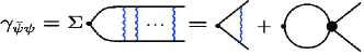
It was found through the previous studies NPRG ; 3dQED that the effective four-fermi operators are found to play an important role for the non-perturbative analysis of the chiral symmetry breaking. The reason may be understood by thinking over the anomalous dimension $\gamma_{\bar{\psi}\psi}$. Fig. 1 shows schematically how the anomalous dimension is represented in terms of the effective four-fermi couplings in the NPRG framework. The four-fermi couplings are also given as a sum of infinitely many loop diagrams by solving the RG equations. Thus a non-perturbative sum of the loop diagrams is carried out by incorporating the four-fermi operators.

Figure 1: The anomalous dimension $\gamma_{\bar{\psi}\psi}$ in terms of the effective four-fermi vertex is shown schematically.

First we consider the Wilsonian effective action of the $SU(N_{c})$ gauge theory with $N_{f}$ massless flavors. The induced operators in the effective action should be invariant under the color $SU(N_{c})$ as well as the flavor symmetry $U(N_{f})_{L}\times U(N_{f})_{R}$. Even if we restrict them to the four-fermi interactions, there are various invariant operators. In order to perform the minimal analysis, we take the following effective Lagrangian,

$${\cal L}_{\rm eff} = -\frac{1}{4g^{2}}{\rm tr}F_{\mu\nu}F^{\mu\nu}+i\sum_{i}\bar{\psi}_{i}D/~{}\psi^{i}$$ (9)

$$-\frac{2G_{S}(\Lambda)}{\Lambda^{2}}\sum_{i,j}\bar{\psi}_{Li}\psi^{j}_{R}\bar{\psi}_{Rj}\psi^{i}_{L}+\cdots,$$

where $i,j=1,\cdots,N_{f}$ denote the flavor indices. In practice, the RG analysis beyond this simple approximation can be also performed. A detailed study of QCD like theories and the gauge-Yukawa theories with many flavors by the NPRG method is reported separately TT . There it is found to be sufficient to incorporate the above four-fermi operator and to sum up the ladder diagrams to examine the IR fixed point.

We should also incorporate higher dimensional operators of the field strength, such as $(D_{\mu}F^{\mu\nu})^{2}$, $(F_{\mu\nu}F^{\mu\nu})^{2}$ and so on in order to extend the gauge beta function beyond the one-loop level. However practical calculations are rather tedious and face with the problem in maintaining the gauge (or BRS) invariance. Therefore we do not deal with the ERG equations faithfully, but substitute the two-loop beta function given by (3) for the RG equation of the gauge coupling instead.

The explicit RG equation for the four-fermi coupling $G_{S}/4\pi^{2}$ is easily found by calculating one-loop diagrams and is given simply by NPRG

$$\Lambda\frac{dg_{S}}{d\Lambda}=2g_{S}-2N_{c}\left(g_{S}+\frac{3}{2}\alpha_{g}\right)^{2},$$ (10)

where we used the Landau gauge propagator. This beta function leads to the fixed points of $g_{S}$ as

$$g_{S}^{*}=\frac{1}{2N_{c}}\left(1-\frac{\alpha_{g}^{*}}{2\alpha_{g,{\rm max}}^{*}}\pm\sqrt{1-\frac{\alpha_{g}^{*}}{\alpha_{g,{\rm max}}^{*}}}\right),$$ (11)

where $\alpha_{g}^{*}$ denotes the gauge coupling $g^{2}/(4\pi)^{2}$ at the fixed point, which is determined by the two-loop beta function (3). The solution with $+(-)$ sign gives the UV (IR) fixed point value. The number represented by $\alpha_{g,{\rm max}}^{*}$ in (11) is the maximal value of the gauge coupling of the fixed point, which is given by

$$\alpha_{g,{\rm max}}^{*}\equiv\frac{g_{\rm max}^{*2}}{(4\pi)^{2}}=\frac{1}{12C_{2}(N_{c})}.$$ (12)

In Fig. 2, the RG flows of $(\alpha_{g},N_{c}g_{S})$ obtained by solving RG equations (3) and (10) are shown in the case of $N_{c}=3$ and $N_{f}=12$. The points A, B and C stand for the non-trivial fixed points of the RG equations. It is seen that the phase boundary appears and all flows in the lower phase approach the IR fixed point A which is the BZ fixed point. It is found that the lower (upper) area of the phase boundary is unbroken (broken) phase of the chiral symmetry NPRG . The phase boundary also shows that the critical gauge coupling of the cutoff gauge theory is given by $\alpha_{g}^{\rm cr}=(g^{\rm cr})^{2}/(4\pi)^{2}\sim 0.09$.

Figure 2: The RG flows of the couplings $(\alpha_{g},g_{S})$ are shown. The IR and the UV fixed points are represented by blob points A and B respectively. The point C stands for the fixed point of the four-fermi theory.

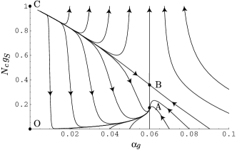
Aspect of the RG flows varies with the flavor number $N_{f}$. When the gauge coupling of the fixed point of the gauge beta function (3) exceeds $\alpha_{g,{\rm max}}^{*}$, then the unbroken phase disappears. Thus the simple RG analysis given above leads to the conformal window of

$$\frac{100N_{c}^{2}-66}{25N_{c}^{2}-15}N_{c}<N_{f}<\frac{11}{3}N_{c},$$ (13)

which coincides with the result obtained from the DS equation in the improved ladder approximation using the two-loop gauge beta function ATW . However we should note also that the lower bound is dependent on the gauge beta function considerably .

In the non-perturbative RG framework, the anomalous dimension of the fermion mass operator $\gamma_{\bar{\psi}\psi}$ is given with the four-fermi coupling as

$$\gamma_{\bar{\psi}\psi}=-6C_{2}(N_{c})\alpha_{g}-2N_{c}g_{S}.$$ (14)

Therefore the explicit value at the BZ fixed point is found to be

$$\gamma_{\bar{\psi}\psi}^{*}=-1+\sqrt{1-\frac{\alpha_{g}^{*}}{\alpha_{g,{\rm max}}}},$$ (15)

which shows that $-1<\gamma_{\bar{\psi}\psi}^{*}<0$ in the conformal window DSanomalous . In the case of $N_{c}=3$ and $N_{f}=12$, $\gamma_{\bar{\psi}\psi}^{*}=-0.8$ $(\alpha_{g}^{*}=0.06<\alpha_{g,{\rm max}}^{*}=0.0625)$, which is fairly close to the critical value.

Now we consider to incorporate the Yukawa interaction given by (2) to the above analysis. Then the scalar exchange diagrams also induce four-fermi operators. However the operators do not contain $\bar{\psi}_{Li}\psi^{j}_{R}\bar{\psi}_{Rj}\psi^{i}_{L}$, but truncated ones such as $\bar{\psi}_{Li}\gamma_{\mu}\psi^{i}_{L}\bar{\psi}_{Rj}\gamma^{\mu}\psi^{j}_{R}$. Thus the RG equation for $g_{S}$ (10) is found to be intact even with the Yukawa interaction except for the anomalous dimension of the fermion $\gamma_{\psi}=\alpha_{\lambda}/2$;

$$\Lambda\frac{dg_{S}}{d\Lambda}=(2+2\alpha_{\lambda})g_{S}-2N_{c}\left(g_{S}+\frac{3}{2}\alpha_{g}\right)^{2}.$$ (16)

We may refer Ref. TT for the detailed analysis. On the other hand, the RG equation for the Yukawa coupling is modified with the four-fermi interaction as

$$\Lambda\frac{d\alpha_{\lambda}}{d\Lambda}=2\alpha_{\lambda}(\gamma_{\phi}+\gamma_{\bar{\psi}\psi}),$$ (17)

where the anomalous dimensions are given explicitly by

$$\gamma_{\phi} = 2N_{c}n_{f}\alpha_{\lambda},$$ (18)

$$\gamma_{\psi} = -6C_{2}(R)\alpha_{g}+\alpha_{\lambda}-2N_{c}g_{S}.$$ (19)

Therefore we may solve the RG equations (3), (16) and (17).

In Fig. 3, the RG flows in the coupling space of $(\alpha_{g},\alpha_{\lambda},N_{c}g_{S})$ are shown in the case of $N_{c}=3,N_{f}=n_{f}=12$. The black points stand for the fixed points. It is seen that the IR fixed point A’ exists and the gauge coupling takes almost the same value as that of the BZ fixed point A. The points B and B’ represent the UV fixed point and the renormalized trajectories linking these fixed points are also shown in Fig. 3.

Figure 3: The RG flows of in the coupling space of $(\alpha_{g},\alpha_{\lambda},N_{c}g_{S})$ are shown. The points A’ and B’ represent the IR and the UV fixed points of the gauge-Yukawa theory respectively, while A and B stand for the BZ (IR) and UV fixed points shown in Fig. 2.

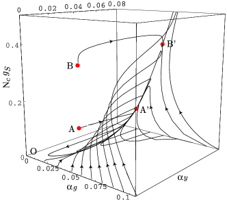
The anomalous dimensions at the IR fixed point may be evaluated as $\gamma_{\phi}^{*}=-\gamma_{\bar{\psi}\psi}^{*}\simeq 0.8$ ($\epsilon=2(1-\gamma_{\phi}^{*})\simeq 0.4$). It is noted that the Yukawa coupling is not extremely large and $\lambda^{*}\simeq 1.3$.

II.4 Effects of the large anomalous dimension

Around the IR fixed point, the scalar potential is renormalized in a peculiar way due to the large anomalous dimension TT . If the scalar potential at the scale $\lambda$ is given as

$$V(\phi)=\tilde{m}_{\phi}^{2}\Lambda^{2}|\phi|^{2}+\frac{\lambda_{4}}{4}|\phi|^{4}+\cdots,$$ (20)

then the RG equations for the dimensionless parameters $\tilde{m}_{\phi}^{2}$ and $\lambda_{4}$ are found to be

$$\Lambda\frac{d\tilde{m}^{2}_{\phi}}{d\Lambda} = -2(1-\gamma_{\phi})\tilde{m}^{2}_{\phi}+4N_{c}n_{f}\alpha_{\lambda}-2\tilde{\lambda}_{4},$$ (21)

$$\Lambda\frac{d\tilde{\lambda}_{4}}{d\Lambda} = 4\gamma_{\phi}\tilde{\lambda}_{4}-8N_{c}n_{f}\alpha_{\lambda}^{2}+\tilde{\lambda}_{4}^{2},$$ (22)

where $\tilde{\lambda}_{4}=\lambda_{4}/(4\pi)^{2}$ and $\gamma_{\phi}=2N_{c}n_{f}\alpha_{\lambda}$.

For the simplicity, we shall discuss the solutions of these equations in the large $N_{c}$ limit, or with neglecting corrections by the quartic coupling $\lambda_{4}$. If we set the Yukawa coupling to the fixed point value, then these equations are easily solved. The solution of the scalar mass at a low energy scale $M$ is given with the initial parameter $\tilde{m}^{2}_{\phi}(\Lambda)$ at the cutoff scale $\Lambda$ and may be written down as

$$m_{\phi}^{2}(M)=\left[\tilde{m}^{*2}_{\phi}+\left(\frac{\Lambda}{M}\right)^{\epsilon}(\tilde{m}^{2}_{\phi}(\Lambda)-\tilde{m}^{*2}_{\phi})\right]M^{2},$$ (23)

where $\tilde{m}_{\phi}^{*2}\equiv 2\gamma_{\phi}^{*}/\epsilon=\gamma_{\phi}^{*}/(1-\gamma_{\phi}^{*})$. It is explicitly seen that the power of divergence is reduced to $\epsilon$ due to the anomalous dimension. As the renormalization scale $\mu$ goes to zero, the scalar mass $m_{\phi}^{2}(\mu)=\tilde{m}_{\phi}^{*2}\mu^{2}$ also goes to zero irrespectively of the initial value $\tilde{m}_{\phi}^{2}(\Lambda)$.

In the next section, we consider a model in which the conformal invariance is terminated at a low energy scale $M$ by adding masses to the fermions. Then the scalar (mass)² may be estimated as $O(1-10)\times M^{2}$. The dependence on the cutoff scale $\Lambda$ as well as the initial parameter is remarkably weaken for a small $\epsilon$. To be explicit, $(\Lambda/M)^{\epsilon}\sim 6.3(2.5)$ for $(\Lambda/M)^{2}=10^{4}(10^{2})$ in the case of $\epsilon=0.4$ ($N_{c}=3,N_{f}=12$).

On the other hand the anomalous dimension makes the quartic coupling highly irrelevant, since the scaling dimension of $\lambda_{4}$ is given by $4\gamma_{\phi}^{*}$ at the IR fixed point. This does not mean that the quartic coupling is eliminated. The RG equation (22) tells us that $\lambda_{4}$ approaches the fixed point value given by

$$\lambda_{4}^{*}\simeq|\lambda^{*}|^{2}=\frac{(4\pi)^{2}}{2N_{c}n_{f}}\gamma_{\phi}^{*},$$ (24)

very strongly. Thus it is found that the value of the quartic coupling $\lambda_{4}$ appearing below the scale $M$ is large in general. Similarly the couplings of higher point interactions of the scalar converge to the fixed point values strongly. The presence of the quartic coupling in the RG equations (21) and (22) does not alter the above properties.

Now we shall move on to the extension of the SM. We introduce a strongly coupled gauge sector in the conformal window other than the SM and also assume that the Higgs field has a Yukawa coupling with this sector just like (2). In order to avoid extreme fine-tuning, scale of the fermion mass $M$, which is the scale of conformal symmetry breaking, should be of O(1)TeV. On the other hand, a large quartic coupling is induced through this Yukawa interaction. Therefore, the observed Higgs mass should be as large as the triviality bound with the cutoff scale $M$. For $M$ of a few TeV, the Higgs mass is expected to be as heavy as 500 GeV KM . Then, the corrections to the Higgs mass through the standard model interactions does not require fine-tuning.

One may wonder if the extra fermions coupled with Higgs field induces so large corrections that contradict with the EW precision measurements. On the other hand, the extra sector should generate a suitable amount corrections to the $S$ and $T$ parameters, as was mentioned in Introduction. We will discuss this phenomenological issue in section IV.

Another problem to be concidered is the mass of Top quark. It is noted that the large anomalous dimension of the Higgs field also suppresses the top Yukawa coupling, which should be about 1 at low energy in order to explain the observed mass. To be explicit, the anomalous dimension of the Higgs $\gamma_{H}^{*}$ suppresses the top Yukawa coupling as

$$y_{t}(\mu)\sim\left(\frac{\mu}{\Lambda}\right)^{\gamma_{H}^{*}}y_{t}(\Lambda).$$ (25)

Then, the top Yukawa coupling must be non-perturbatively large immediately above the TeV scale. Therefore we have to replace the strongly coupled conformal sector so as to include the top quarks. In general, scenarios of the EWSB with the Higgs field coupled to the strongly interacting sector, such as the walking Technicolor models walkingTC , the conformal Technicolor models LO and so on, seem to face with a similar problem in compatibility with the top quark mass .

In the next section, we consider a model, in which the top Yukawa coupling is generated through mixing between top quarks and the fermions in the CFT sector coupled strongly with the Higgs KNT . On the way around, such a mixing effect may explain origin of the prominently large top quark mass.

III A phenomenological model

Now we shall consider an explicit phenomenological realization of the mechanism discussed in the previous section, namely the conformal Higgs model. We assume a strongly coupled gauge theory with the gauge group of $SU(3)_{\rm CFT}$ as the conformal sector. The Higgs field couples with the vector-like fermions of the CFT and behaves as a point-like particle below a certain high energy scale $\Lambda$. Here we do not think about the ultraviolet completion above the cutoff scale $\Lambda$, though the Higgs field may be generated as a fermion composite at this scale. The basic feature of the scenario is that the EW symmetry is not broken by the strong dynamics, but by the vacuum expectation value (VEV) of the point-like Higgs. The dynamics of the CFT sector plays a role in suppressing the mass scale of the Higgs boson.

The color gauge group of the SM, $SU(3)_{C}$, emerges after spontaneous symmetry breaking (SSB) of $SU(3)_{\rm CFT}\otimes SU(3)^{\prime}_{C}$ at the TeV scale. The quark fields are charged under $SU(3)^{\prime}_{C}$, while the vector-like fermions are charged under $SU(3)_{\rm CFT}$. These fermions can mix with each other below the scale of SSB, since both fermions are charged under the color gauge group $SU(3)_{C}$. Then a large top Yukawa coupling is induced through the mass mixing between quarks and the colored heavy fermions from the CFT sector.

Explicitly, we will discuss the case in which mixing between the weak doublets, $\Phi_{L}$ and $Q_{3L}$, and between the weak singlet $\phi_{R}$ and $u_{3R}$ occurs dynamically. One may suppose that similar mixing among all flavors of quarks and leptons also occurs and, moreover, the differences in these mixings explain the mass hierarchy. However the mixing in the other quarks than the top quarks should be small anyway, and we neglect them completely in this paper.

We also introduce another gauge interaction of the group $G_{\rm DSB}$, which becomes strong at the TeV scale and breaks down the conformal symmetry by through fermion condensations. The dynamics of the CFT is not influenced above the TeV scale, since the gauge coupling of $G_{\rm DSB}$ sector is rather weak there. However, this dynamics induces masses of the extra fermions of the CFT sector and mixing with the quarks simultaneously at the TeV scale.

We assume that $G_{\rm DSB}$ is also an $SU(3)$ group and introduce the following vector-like fermions charged as,

$$\begin{array}[]{c|ccccc}&SU(3)_{\rm DSB}&SU(3)_{\rm CFT}&SU(3)_{C}^{\prime}&SU(2)_{W}&U(1)_{Y}\\ \hline\cr\psi^{A}&\mbox{\bf 3}&\mbox{\bf 3}&\mbox{\bf 1}&\mbox{\bf 1}&\mbox{any}\\ \eta^{a}&\mbox{\bf 3}&\mbox{\bf 1}&\mbox{\bf 3}&\mbox{\bf 1}&\mbox{any}\\ \hline\cr\Phi^{iA}&\mbox{\bf 1}&\mbox{\bf 3}&\mbox{\bf 1}&\mbox{\bf 2}&1/6\\ \phi^{iA}&\mbox{\bf 1}&\mbox{\bf 3}&\mbox{\bf 1}&{\bf 1}&2/3\end{array}$$ (26)

where $A=1,2,3$ and $a=1,2,3$ stand for indices of $SU(3)_{\rm CFT}$ and $SU(3)_{C}^{\prime}$ respectively. Another suffix $i$ runs $1,2,3$. Then the $SU(3)_{\rm CFT}$ gauge sector may be regarded as a gauge theory with $N_{c}=3$ and $N_{f}=12$. Therefore an IR fixed point appears at the fairly strong coupling region. The assignment of the $U(1)_{Y}$ hypercharges for $\Phi$ and $\phi$ allows mixing with the up-sector quarks.

The Higgs field is allowed to have the following Yukawa interactions,

$$-{\cal L}_{\rm Yukawa} = Y_{t}\bar{Q}_{3L}u_{3R}\tilde{H}+Y_{b}\bar{Q}_{3L}d_{3R}H$$ (27)

$$+\lambda\sum_{i}\bar{\Phi}_{iA}\phi^{iA}\tilde{H},$$

where $\tilde{H}=\epsilon_{ab}H^{b*}$ as in the SM Lagrangian and we omitted quarks in the first and second generations. For the sake of simplicity, we suppose the coupling $\lambda$ to be the IR fixed point value $\lambda_{*}$ at the scale of $\Lambda$ already. The explicit value of $\lambda_{*}$ may be estimated from Eq. (17) by noting the number of flavors coupled with the Higgs is $n_{f}=3$, and found to be about $2.65$. We will also neglect the Yukawa couplings of the third generation $Y_{t}$ and $Y_{b}$ for a while, since these couplings are suppressed by the anomalous dimension of the Higgs field.

The gauge interaction of $SU(3)_{\rm DSB}$ induces condensation of fermion bilinears such as $\langle\bar{\psi}_{A}\cdot\psi^{A}\rangle$ and $\langle\bar{\eta}_{a}\cdot\eta^{a}\rangle$ at low energy, where $\cdot$ represents $SU(3)_{\rm DSB}$-singlet contraction. The symmetry breaking of $SU(3)_{\rm CFT}\otimes SU(3)_{C}^{\prime}$ to $SU(3)_{C}$ also takes place, if the diagonal components of the composite fields acquire non-vanishing VEVs as

$$\langle\bar{\psi}_{A}\cdot\eta^{a}\rangle\equiv\langle\Omega_{A}^{a}\rangle\propto\delta_{A}^{a},~{}\langle\bar{\eta}_{a}\cdot\psi^{A}\rangle\equiv\langle\bar{\Omega}^{A}_{a}\rangle\propto\delta_{a}^{A}.$$ (28)

On the other hand, the effective Lagrangian given at the scale $\Lambda$ may contain the non-renormalizable interactions such as

$$- {\cal L}_{\rm four-fermi}$$ (29)

$$= \frac{c}{\Lambda^{2}}\bar{Q}_{3La}\Phi^{3A}_{R}(\bar{\psi}_{A}\cdot\eta^{a})+\frac{\bar{c}}{\Lambda^{2}}\bar{\phi}_{3A}u_{R}^{3a}(\bar{\eta}_{a}\cdot\psi^{A})$$

$$+\frac{c_{\Phi}}{\Lambda^{2}}\bar{\Phi}_{iA}\Phi^{iA}(\bar{\eta}_{a}\cdot\eta^{a})+\frac{c_{\phi}}{\Lambda^{2}}\bar{\phi}_{iA}\phi^{iA}(\bar{\eta}_{a}\cdot\eta^{a}).$$

The coefficients of the four-fermi interactions are unknown, unless the ultraviolet completion of the model at the scale $\Lambda$ is fixed. In any case, their explicit values are unimportant in the following argument. However, we assumed here that only the third generation quarks have four-fermi interactions with sizable couplings with some reason. Otherwise large Yukawa couplings are induced to all flavors as well as top quark through mixing effect discussed below.

Thus the low energy effective interactions obtained after the symmetry breaking may be reduced to the form of

$$-{\cal L}_{\rm int} = \lambda_{*}(\bar{\Phi}_{iL}\phi_{R}^{i}+\bar{\Phi}_{iR}\phi_{L}^{i})\tilde{H}+V(H)$$ (30)

$$+M_{\Phi}\left(\bar{\Phi}_{3L}+\frac{\omega}{M_{\Phi}}\bar{Q}_{3L}\right)\Phi_{R}^{3}$$

$$+M_{\phi}\bar{\phi}_{3L}\left(\phi_{R}^{3}+\frac{\bar{\omega}}{M_{\phi}}u_{R}^{3}\right),$$

where we defined the parameters $\omega$ and $\bar{\omega}$ by the VEV of SSB as $c\langle\Omega_{A}^{a}\rangle/\Lambda^{2}=\omega\delta_{A}^{a}$ and $\bar{c}\langle\bar{\Omega}^{A}_{a}\rangle/\Lambda^{2}=\bar{\omega}\delta_{a}^{A}$. The mass parameters $M_{\Phi}$ and $M_{\phi}$ are also generated through the fermion condensation $\langle\bar{\eta}_{a}\cdot\eta^{a}\rangle$ and give the decoupling scale of the extra sectors from the SM. Naively these mass parameters are supposed to be of the same order as $\omega$ and $\bar{\omega}$. In the above argument, we did not take account of the fermion condensation of $\langle\bar{\psi}_{A}\cdot\psi^{A}\rangle$ intentionally, since there are subtle dynamical issues. We shall discuss the issues in the end of this section.

Now it is apparent from the effective Lagrangian (30) that mixing occurs between the quark fields and the extra matter fields. Note that this mixing respects the EW gauge symmetry, since the SSB does not break the EW symmetry. The mixing appears between the left-handed doublets, $Q_{3L}3$ and $\Phi_{3L}$, and also between the right-handed singlets, $u_{3R}$ and $\phi_{3R}$. The mass eigenmodes are explicitly given as

$$\left(\begin{array}[]{c}Q_{3}^{\prime}\\ \Phi_{3}^{\prime}\end{array}\right)_{L} = \left(\begin{array}[]{cc}\cos\theta_{L}&\sin\theta_{L}\\ \sin\theta_{L}&\cos\theta_{L}\end{array}\right)\left(\begin{array}[]{c}Q_{3}\\ \Phi_{3}\end{array}\right)_{L},$$ (37)

$$\left(\begin{array}[]{c}u_{3}^{\prime}\\ \phi_{3}^{\prime}\end{array}\right)_{R} = \left(\begin{array}[]{cc}\cos\theta_{R}&\sin\theta_{R}\\ \sin\theta_{R}&\cos\theta_{R}\end{array}\right)\left(\begin{array}[]{c}u_{3}\\ \phi_{3}\end{array}\right)_{R},$$ (44)

where the mixing angles $\theta_{L}$ and $\theta_{R}$ are given by $\tan\theta_{L}=\omega/M_{\Phi}$ and $\tan\theta_{R}=\bar{\omega}/M_{\phi}$ respectively. Then the effective interaction Lagrangian is rewritten in terms of these mass eigenmodes as

$$- {\cal L}_{\rm int}$$ (45)

$$= \lambda_{*}(\cos\theta_{L}\bar{\Phi}^{\prime}_{3L}-\sin\theta_{L}\bar{Q}^{\prime}_{3L})(\cos\theta_{R}\phi_{3R}^{\prime}-\sin\theta_{R}u^{\prime}_{3R})\tilde{H}$$

$$+\lambda_{*}\bar{\Phi}_{3R}\phi_{3L}\tilde{H}+M_{\Phi}^{\prime}\bar{\Phi}^{\prime}_{3L}\Phi_{3R}+M_{\phi}^{\prime}\bar{\phi}_{3L}\phi_{3R}^{\prime}$$

$$+V(H),$$

where masses of the eigenmodes are given by $M_{\Phi}^{\prime}=M_{\Phi}/\cos\theta_{L}$ and $M_{\phi}^{\prime}=M_{\phi}/\cos\theta_{R}$. The massless top quarks are identified with $(Q^{\prime}_{3L},u^{\prime}_{3R})$, and their effective Yukawa coupling with the Higgs field turns out to be

$$Y_{t}^{\rm eff}\sim\lambda_{*}\sin\theta_{L}\sin\theta_{R}.$$ (46)

This coupling can be large enough, unless the mixing angles, or the ratios $\omega/M$, are very small, since the fixed point coupling $\lambda_{*}$ is large in this model.

Thus the Higgs mass may be suppressed by the conformal dynamics in a way compatible with the large top Yukawa coupling. However there are some issues to be concerned about in the conformal Higgs model. First one may wonder whether the $SU(3)_{\rm DSB}$ interaction affects the IR fixed point and, moreover, may destroy the conformal invariance fairly above the decoupling scale. Indeed the conformal invariance is not exact, but the beta function of the CFT gauge coupling is affected by the DSB gauge coupling $\alpha_{g^{\prime}}$ at the two-loop level as

$$\mu\frac{d\alpha_{g}}{d\mu}=\cdots+4\alpha_{g}^{2}\alpha_{g}^{\prime}.$$ (47)

Then the fixed point coupling is shifted to $\alpha_{g}^{*}\sim(b_{0}-2\alpha_{g}^{\prime})/b_{1}$ effectively. However the DSB sector may be regarded as an $N_{c}=3$ and $N_{f}=6$ QCD and $\alpha_{g^{\prime}}$ becomes comparable with $\alpha_{g}^{*}$ very near the dynamical scale $M_{\Phi}$. Therefore the shift of the IR fixed point is very small.

We should also think about effects to the four-fermi couplings, since the DSB gauge interaction increases attractive force among the fermions $\psi^{A}$ in the CFT sector. In practice, the effective four-fermi interactions among the fermion $\psi$ are induced. In the above model, however, the gauge coupling of the IR fixed point is already close to the critical value $\alpha_{g,{\rm max}}$ without the DSB interaction. Therefore the RG flow of the four-fermi coupling enters the broken phase eventually, although the running near the boundary is rather slow . However note that the DSB gauge interaction does not affect the four-fermi interactions among $\Phi$ and $\phi$ directly. The beta function for the four-fermi coupling $g_{S}$ (10) is unchanged in the ladder or the large $N_{c},N_{f}$ leading approximation. Thus it is thought that the IR fixed point is not shifted remarkably or destroyed through the DSB gauge interaction.

Next we also consider effects of the large anomalous dimension on the scale of dynamically generated masses. The four-fermi interactions given in the effective Lagrangian (29) are also enhanced by the anomalous dimensions due to $SU(3)_{\rm CFT}$ interaction, since they include the fermions of the CFT sector,$\psi$, $\Phi$ and $\phi$. This effect enlarges the scale of dynamical masses . For example, the mass parameters $M_{\Phi}$ $(M_{\phi})$ and $\omega$ $(\bar{\omega})$ are estimated in terms of the dynamical scale $M_{\rm DSB}$ of the DSB interaction as

$$M_{\Phi}\sim\omega\sim\left(\frac{M_{\rm DSB}}{\Lambda}\right)^{2+\gamma_{\bar{\psi}\psi}^{*}}M_{\rm DSB}.$$ (48)

Thus the extra matter fields in the CFT are decoupled at the mass scale $M_{\Phi}$ and $M_{\phi}$, which are relatively larger than the dynamical symmetry breaking scale $M_{\rm DSB}$. Therefore the strong dynamics of the CFT is not responsible for the EW symmetry breaking, but solely reduces the radiative corrections to the Higgs mass parameter.

Provided that the effective Lagrangian also contains the four-fermi coupling as

$$\frac{\tilde{c}_{\Phi}}{\Lambda^{2}}\bar{\Phi}_{iA}\Phi^{iA}(\bar{\psi}_{A}\cdot\psi^{A}),$$ (49)

then the fermion condensation $\langle\bar{\psi}_{A}\cdot\psi^{A}\rangle$ generates the mass $\hat{M}_{\Phi}$ to the fermion $\Phi$, which is enhanced as

$$\hat{M}_{\Phi}\sim\left(\frac{M_{\rm DSB}}{\Lambda}\right)^{\gamma_{\bar{\psi}\psi}^{*}}M_{\Phi}\gg M_{\Phi}.$$ (50)

Then the decoupling mass scale is determined by $\hat{M}_{\Phi}$ instead of $M_{\Phi}$. Consequently the mixing angle is reduced to be $\omega/\hat{M}_{\Phi}\ll 1$ and, therefore, the induced top Yukawa coupling turns out to be too small. This is the reason why we did not include the interaction of (49) in the effective Lagrangian (29). We need to assume the coefficient $\hat{c}_{\Phi}$ of the four-fermi operator (49) to be suppressed with some reason.

IV The Electro-Weak precision tests

IV.1 Oblique corrections

New interactions above the TeV scale, which is required to push up the cutoff scale of the EW theory to some higher scale, must be consistent with the precision tests of the EW theory by the LEP experiments. Especially the oblique corrections to the EW gauge bosons put rather strong constraints to the S and T parameters. In this subsection we shall evaluate these parameters in the conformal Higgs model presented in the previous section.

It has been known for some time that QCD-like gauge theories induce an excessive correction to the S-parameter PT ; strongEW . Although it is a difficult dynamical problem to evaluate the oblique corrections in general strong dynamics, there have been also some studies by using the DS equations. According to the recent study HKY , the S-parameter is decreased in the walking Technicolor models walkingTC compared with QCD-like models, however seems to be still large. Thus models with dynamical EW symmetry breaking seem to have a potential difficulty in satisfying the EW precision tests. Contrary to this, neither the CFT interaction nor the DSB interaction does not induce the EW symmetry breaking in the present scenario. Therefore the huge correction to the S-parameter is not generated through the strong dynamics. This point is the essential difference from e.g. the walking Technicolor walkingTC and the conformal Technicolor LO .

However the extra fermions $\Phi$ and $\phi$ couple with the Higgs field. Moreover the weak isospin symmetry is largely broken, since these fermions mix only with the top quark fields. Therefore a sizable correction to the $\rho$ parameter, or the T-parameter, may be generated through loop effect of these extra fermions.

The oblique corrections are generated through mixing among the EW doublet and the EW singlet fields after the EWSB. Explicitly, the VEV of the Higgs field, $\langle H\rangle=(0,v/\sqrt{2})$ leads the mass terms given by

$$\left(\begin{array}[]{ccc}\bar{t}_{L}&\bar{\chi}^{\prime}_{1L}&\bar{\phi}_{L}\end{array}\right)\left(\begin{array}[]{ccc}\lambda_{*}\sin\theta_{L}\sin\theta_{R}v/\sqrt{2}&0&-\lambda_{*}\sin\theta_{L}\cos\theta_{R}v/\sqrt{2}\\ -\lambda_{*}\cos\theta_{L}\sin\theta_{R}v/\sqrt{2}&M^{\prime}_{\Phi}&\lambda_{*}\cos\theta_{L}\cos\theta_{R}v/\sqrt{2}\\ 0&\lambda_{*}v/\sqrt{2}&M^{\prime}_{\phi}\end{array}\right)\left(\begin{array}[]{c}t_{R}\\ \chi_{1R}\\ \phi^{\prime}_{R}\end{array}\right)$$ (58)

$$+M^{\prime}_{\Phi}\bar{\chi}_{2L}\chi_{2R}+\mbox{\it h.c.},$$ (59)

where the component fields are defined by $Q^{\prime}_{3L}=(t,b)_{L}$, $u^{\prime}_{3R}=t_{R}$, $\Phi^{\prime}_{L}=(\chi^{\prime}_{1},\chi^{\prime}_{2})_{L}$ and $\Phi_{R}=(\chi_{1},\chi_{2})_{R}$. Since the VEV for the EWSB $v$ is much smaller than $M_{\Phi}$ and $M_{\phi}$, the top quark mass $m_{t}$ is given almost by $\lambda_{*}\sin\theta_{L}\sin\theta_{R}v/\sqrt{2}=Y_{t}^{\rm eff}v/\sqrt{2}$. Therefore the mixing angles should satisfy $\sin\theta_{L}\sin\theta_{R}\sim 1/\lambda_{*}$. If we suppose $\bar{\omega}\sim\omega$ and $M_{\Phi}\sim M_{\phi}\sim M$ for simplicity, the mixing angles in the explicit model should satisfy

$$\sin\theta_{L}\sim\sin\theta_{R}\sim 1/\sqrt{\lambda_{*}}\sim 0.6.$$ (60)

Now mixing among the EW doublets and singlets is induced through diagonalization of the mass matrix given by (59). The mixing decreases in proportion to $v/M$ for a large $M$, as is seen from the mass matrix. Therefore the oblique corrections are also vanishing for a sufficiently large $M$. This is because the dynamically induced masses of $M$ for the extra matter fields are invariant under the EW symmetry, and these fields just decouple from the EW sector. On the other hand, small but suitable amounts of oblique corrections should be induced so that the heavy Higgs boson is compatible with the EW precision tests. Thus the decoupling scale of the CFT sector $M$ can be determined by this phenomenological consistency. However, the scale $M$ should be relatively low in order to improve naturalness of the EW theory. Therefore it is important to see whether the conformal Higgs model really allows the decoupling scale less than a few TeV.

Now let us evaluate $\Delta T$ by calculating the one-loop corrections for the self-energy of the EW gauge bosons. In practice, the explicit model is very similar to the top seesaw models topseesaw as far as the mixing mechanism is concerned, while the top quark mass is not generated through the seesaw mechanism. So we may evaluate the oblique corrections in the same manner as done for the top seesaw models. More explicitly, the oblique corrections induced by vectorlike fermions given in Ref. loopcorr are also available.

Since the required corrections are small somehow, we may consider only the cases with $\lambda_{*}v\ll M_{\Phi},M_{\phi}$. Then the mass terms given by (59) can be approximated as

$$m_{t}\bar{t}_{L}t_{R}+M^{\prime}_{\Phi}\bar{\chi}^{\prime}_{1L}\left(\chi_{1R}-\frac{\lambda_{*}v}{\sqrt{2}M^{\prime}_{\Phi}}\cos\theta_{L}\sin\theta_{R}t_{R}\right)$$

$$+M^{\prime}_{\phi}\left(\bar{\phi}_{L}-\frac{\lambda_{*}v}{\sqrt{2}M^{\prime}_{\phi}}\sin\theta_{L}\cos\theta_{R}\bar{t}_{L}\right)\phi^{\prime}_{R}.$$ (61)

It is seen that we need to take account of both mixings between the left-handed fermions $(t_{L},\phi_{L})$ and between the right-handed fermion $(t_{R},\chi_{1R})$.

The contribution through the mixing of the left-handed fermions is found to be

$$\Delta T\sim\frac{3}{16\pi^{2}\alpha v^{2}}\left\{2m_{t}^{2}\ln\frac{{M^{\prime}}^{2}_{\phi}}{m_{t}^{2}}+x_{L}^{2}\right\}\left(\frac{x_{L}}{M^{\prime}_{\phi}}\right)^{2},$$ (62)

where $x_{L}=\lambda_{*}\sin\theta_{L}\cos\theta_{R}v/\sqrt{2}$. In this expression, the fine structure constant $\alpha$ may be evaluated as $\alpha^{-1}(M_{Z})\sim 129$. Similarly, the contribution through the mixing of the right-handed fermions are found to be

$$\Delta T\sim\frac{3}{16\pi^{2}\alpha v^{2}}x_{R}^{2}\left(\frac{x_{R}}{M^{\prime}_{\Phi}}\right)^{2},$$ (63)

where $x_{R}=\lambda_{*}\cos\theta_{L}\sin\theta_{R}v/\sqrt{2}$. Thus both contributions by the heavy extra quarks are positive.

If we take simply $M^{\prime}_{\Phi}\simeq M^{\prime}_{\phi}\simeq M$ and $x_{L}\simeq x_{R}\simeq x$, the total correction of $\Delta T$ is approximately given by

$$\Delta T\sim\frac{3}{16\pi^{2}\alpha}\left\{\ln\frac{M^{2}}{m^{2}_{t}}+\frac{x^{2}}{m^{2}_{t}}\right\}\left(\frac{x}{M}\right)^{2},$$ (64)

where we used $2m^{2}_{t}\simeq v^{2}$. Here the parameter $x$ is not free but is related with the fixed point Yukawa coupling $\lambda_{*}$ as

$$x^{2}\simeq m^{2}_{t}\left(\frac{1}{\sin^{2}\theta}-1\right)\simeq m^{2}_{t}(\lambda_{*}-1).$$ (65)

If this oblique correction supplies $\Delta T=0.25\pm 0.1$ additionally to the SM correction, then the heavy Higgs mass of $400-600$GeV becomes consistent with the current evaluation of the EWPT LEP ; heavyhiggs . If we substitute $\lambda_{*}=2.63$ into $\Delta T$ given by Eq. (64), then the decoupling mass scale may be determined to be

$$1.5\mbox{TeV}<M<2.5\mbox{TeV}.$$ (66)

It is noted that the consistent scale $M$ can appear at a relatively low energy region. This is because that the fixed point Yukawa coupling $\lambda_{*}$ is not very large in the explicit model. Therefore, the amount of induced oblique correction is model dependent.

Similarly, contribution to the S-parameter may be evaluated and is found to be

$$\Delta S\leq\frac{1}{\pi}\ln\frac{M^{2}}{m^{2}_{t}}\left(\frac{x}{M}\right)^{2}.$$ (67)

This is much smaller than the contribution to $\Delta T$, since

$$\frac{\Delta S}{\Delta T}\leq\frac{16\pi}{3}\alpha\simeq 0.12.$$ (68)

This property is common with the top see-saw models topseesaw . Thus the S-parameter is also consistent with the EWPT. Here, we should say that these one-loop analysis of the oblique correction is not so definite indeed. The higher order corrections by the QCD interaction are not be negligible. The CFT fermions also interact with the massive gauge bosons rather strongly. However such corrections are thought to be suppressed, since the gauge boson mass is so heavy as the decoupling scale $M$. Therefore ambiguity of the one-loop analysis would not be so large. In any case, it seems that the present model with the decoupling scale of a few TeV is viable.

IV.2 Z-boson decay width

The EW precision tests also constrain the ratio of decay widths of Z-boson, $R_{b}\equiv\Gamma[Z\rightarrow b\bar{b}]/\Gamma[Z\rightarrow\mbox{hadrons}]$ severely. The deviation of coupling between the bottom quark and Z-boson $g_{b}$ from the SM value, $\delta g_{b}$, is restricted roughly as $\delta g_{b}<10^{-3}$. Theoretically, this deviation can be also induced through mixing between bottom quarks and the massive extra fermions. Indeed there are such mixings in the explicit model and $\delta R_{b}$ should be examined.

So far we have ignored the original top and bottom Yukawa couplings, since these are suppressed and not important to other effects. However we should add the bottom Yukawa term $y_{b}\bar{Q}_{3L}b_{R}H$ to the effective Lagrangian given by (30) in order to see the mixing effect. The original top and bottom Yukawa terms are rewritten in terms of the mass eigenmodes into

$$-{\cal L}_{\rm Yukawa} = y_{t}(\sin\theta_{L}\bar{\Phi}^{\prime}_{L}+\cos\theta_{L}\bar{Q}^{\prime}_{3L})t_{R}\tilde{H}$$ (69)

$$+y_{b}(\sin\theta_{L}\bar{\Phi}^{\prime}_{L}+\cos\theta_{L}\bar{Q}^{\prime}_{3L})b_{R}H.$$

Therefore the EWSB induces the mixed mass terms given by

$$\left(\begin{array}[]{cc}\bar{b}_{L}&\bar{\chi}^{\prime}_{2L}\end{array}\right)\left(\begin{array}[]{ccc}y_{b}\cos\theta_{L}v/\sqrt{2}&0\\ y_{b}\sin\theta_{L}v/\sqrt{2}&M^{\prime}_{\Phi}\end{array}\right)\left(\begin{array}[]{c}b_{R}\\ \chi_{2R}\end{array}\right)+\mbox{\it h.c.}.$$ (70)

Then it is shown that both of $b_{L}$ and $b_{R}$ are mixed with components of the weak doubles fermions $\Phi_{L}$ and $\Phi_{R}$ through the EWSB. Both of the $Zb_{L}\bar{b}_{L}$ and $Zb_{R}\bar{b}_{R}$ couplings induced the mixing effect are readily evaluated, since these are tree level contributions. The deviations are found to be

$$\delta g_{bL}\simeq\delta g_{bR}\simeq\left(\frac{m_{b}}{M}\right)^{2}\leq 10^{-5},$$ (71)

which are sufficiently small. Similarly, we may estimate the deviations in the couplings of top quarks. They are given roughly as $\delta g_{tL}\simeq\delta g_{tR}\leq 10^{-2}$.

IV.3 Aspect of fine-tuning

As is explained before this scenario leads to a relatively heavy Higgs. The mass is close to the triviality bound corresponding with the scale $M$, which are approximately $400-600$ GeV Then the SM correction to the Higgs mass parameter becomes comparable with such a heavy mass itself, when the scale $M$ of a few TeV acts as the cutoff scale. Thus the fine-tuning due to the SM corrections is not necessary.

Then, we should think about corrections to the Higgs mass parameter by the CFT dynamics. Indeed the Higgs mass is suppressed by the anomalous dimension, however the correction is sizable compared with the EW scale. As was discussed in section II, the Higgs (mass)² at the decoupling scale $M$ is given as Eq. (23). This may be estimated as $O(1-10)\times M^{2}$, which is too large to bring about the Higgs mass of $400-600$ GeV. Thus the initial mass parameter must be tuned somehow. Since the degree of the fine-tuning BG is given roughly as

$$\Delta=\frac{m_{H}^{2}(\Lambda)}{\tilde{m}_{H}^{2}(M)}\frac{\delta\tilde{m}_{H}^{2}(M)}{\delta m_{H}^{2}(\Lambda)}\sim\ln\left(\frac{\Lambda^{2}}{M^{2}}\right)\frac{M^{2}}{\tilde{m}_{H}^{2}(M)},$$ (72)

it is found that fine-tuning of $O(1)$ % is still necessary in order to achieve the realistic EWSB for the cutoff scale $\Lambda$ of, say, $O(100)TeV$. Of course this cutoff scale cannot be taken extremely high. The model should be also replaced with some new physics, which probably does not contain the elementary Higgs field. However we do not discuss the ultraviolet completion of the present model in this paper and postpone it to future study.

V Conclusions and discussions

In this paper we discussed a new scenario in which the quadratic correction to the Higgs mass parameter is suppressed by a large anomalous dimension endowed by interactions with a CFT sector. With this mechanism, the cutoff scale can be raised up sufficiently high so as to solve the so-called little hierarchy problem of the SM. The strong dynamics of the CFT sector does not break the EW symmetry, but radiative symmetry breaking of the Higgs field as in the supersymmetric theories takes place. The CFT sector just decouples from the SM sector by dynamical mass generation at a few TeV scale.

It was shown explicitly that a large anomalous dimension of the Higgs field can be realized in a class of the gauge-Yukawa theories. We analyzed the non-perturbative RG equations to show it. The quartic coupling of the Higgs fields is rendered very irrelevant by the anomalous dimension and converges to a fixed point value. Due to strong dynamics of the CFT sector, this fixed point coupling is rather large. Therefore the scenario predicts a fairly heavy mass for the SM Higgs, which contrasts with the supersymmetric models and the little Higgs models.

The anomalous dimension of the Higgs field suppresses the Yukawa couplings in the SM as well. Then compatibility with the large top quark mass becomes problematic. We considered an explicit model, which we called “the conformal Higgs model”, solving this problem due to mixing with top quark and the extra fermions of the CFT sector.

The heavy Higgs boson is not consistent with the EWPT of the $(S,T)$ parameters, unless a suitable amount of extra contribution is added. However the mixing with the CFT fermions is found to induce a proper oblique corrections in the conformal Higgs model, if their mass scale is given to be a few TeV. Therefore the model predicts extra heavy colored fermions and massive $SU(3)_{C}$ gauge bosons with a few TeV masses. Correction to the decay width of Z-boson due to the mixing effect is negligible. Thus such extension of the SM also seems viable phenomenologically.

The anomalous dimension of the Higgs field may help to raise up the cutoff scale significantly. However the model does not explain the scale of EWSB in general. Naively the decoupling scale of a few TeV gives also the Higgs mass scale. Therefore the mass parameter must be tuned somewhat, although the Higgs boson is fairly heavy. So the aspect of naturalness is not very satisfactory, and some improvement may be desired. Meanwhile, the minimal supersymmetric SM also requires a similar degree of fine-tuning lowsusy ; fathiggs .

Lastly we also mention further problems to be considered. In the conformal Higgs model, the Higgs boson is assumed to be point-like at least up to some cutoff scale $\Lambda$. However this scale cannot be taken extremely high, and the ultra-violet completion of the model should be considered. One of the possible scenarios would be a composite Higgs model. It was also simply assumed that only top quark is mixed with the extra fermions through the Yukawa interactions. It may be interesting to see whether the mixing effect can be extended to other quarks/leptons than top quark.

It seems also interesting to give a five-dimensional description of the conformal Higgs model, which is suggested by the AdS/CFT correspondence AdS/CFT . The gauge structure of $SU(3)_{\rm CFT}\otimes SU(3)_{C}^{\prime}$ and it’s spontaneous breaking to the diagonal subgroup $SU(3)_{C}$ indicates a two-site deconstruction of a five-dimensional model. Indeed, the vector-like extra fermions may be identified with the first Kaluza-Klein mode of the bulk top quark. Moreover the massive gauge boson may be regarded as the Kaluza-Klein mode of gluon in the bulk. Study in this direction is now under way and the results will be reported elsewhere.

References

- (1) The LEP Collaborations ALEPH, DELPHI, L3, OPAL, and the LEP Electroweak Working Group, hep-ex/0511027.
- (2) B. Grinstein and M.B. Wise, Phys. Lett. B 265, 326 (1991).
- (3) R. Barbieri and A. Strumia, hep-ph/0007265; Phys. Lett. B 462, 144 (1999); R. Barbieri, A. Pomarol, R. Rattazi and A. Strumia, Nucl.Phys.B703:127-146,2004; for a review, for example, see R. Barbieri, hep-ph/0312253.
- (4) N. Arkani-Hamed, A.G. Cohen and H. Georgi, Phys. Lett. B 513, 232 (2001); N. Arkani-Hamed, A.G. Cohen, E. Katz, A.E. Nelson, T. Gregoire and J.G. Wacker, JHEP 0208, 021 (2002); N. Arkani-Hamed, A.G. Cohen, E. Katz and A.E. Nelson, JHEP 0207, 034 (2002); For a review, for example, see M. Schmaltz and D. Tucker-Smith, hep-ph/0502182 and references therein.
- (5) A. Brignole, J.A. Casas, J.R. Espinosa and I. Navarro, Nucl. Phys. B 666, 105 (2003); J.A. Casas, J.R. Espinosa and I. Hidalgo, JHEP 0401 008 (2004).
- (6) P. Batra, A. Delgado, D.E. Kaplan and T.M. P. Tait, JHEP 0402, 043 (2004); JHEP 0406, 032 (2004).
- (7) R. Harnik, G.D. Kribs, D.T. Larson and H. Murayama, Phys. Rev. D70 (2004) 015002; S. Chang, C. Kilic and R. Mahbubani, Phys. Rev. D71 (2005) 015003; A. Birkedal, Z. Chacko and Y. Nomura, Phys. Rev. D71, 015006 (2005); A. Delgado and T.M.P. Tait, JHEP 0507, 023 (2005).
- (8) P.J. Fox, A.E. Nelson and N. Weiner, JHEP 0208 (2002) 035; Z. Chacko, P.J. Fox and H. Murayama, Nucl. Phys. B 706, 53 (2005).
- (9) A. Birkedal, Z. Chacko and M.K. Gaillard, JHEP 0410, 036 (2004); P.H. Chankowski, A. Falkowski, S. Pokorski and J. Wagner, Phys. Lett. B 598, 252 (2004); Z. Berezhiani, P.H. Chankowski, A. Falkowski and S. Pokorski, arXiv:hep-ph/0509311; T. Roy and M. Schmaltz, JHEP 0601, 149 (2006); C. Csáki, G. Marandella, Y. Shirman and A. Strumia, Phys. Rev. D 73, 035006 (2006).
- (10) T. Kobayashi and H. Terao, JHEP 0407, 026 (2004). T. Kobayashi, H. Nakano and H. Terao, Phys. Rev. D71 (2005) 115009 T. Kobayashi, H. Terao and A. Tsuchiya, Phys. Rev. D74 (2006) 015002.
- (11) M.B. Einhorn, D.R.T. Jones and M.J.G. Veltman, Nucl. Phys. B 191, 146 (1981); M.E. Peskin and J.D. Wells, Phys. Rev. D 64, 093003 (2001).
- (12) R. Barbieri, L.J. Hall and V.S. Rychkov, Phys. Rev. D 74, 015007 (2006).
- (13) M.E. Peskin and T. Takeuchi, Phys. Rev. Lett. 65, 964 (1990); Phys. Rev. D 46, 381 (1992).
- (14) For a review, see for example T.L. Barklow et. al., hep-ph/9704217; C.T. Hill and E.H. Simmons, Phys. Rept. 381, 235 (2003); Erratum-ibid. 390, 553 (2004) and references therein.
- (15) C.F. Kolda and H. Murayama, JHEP 0007,035 (2000).
- (16) J.A. Casas, J.R. Espinosa and I. Hidalgo, arXiv:hep-ph/0607279.
- (17) M. A. Luty and T. Okui, JHEP 0609 (2006) 070.
- (18) For a review from phenomenological point of view, see for instance C. Csaki, J. Hubisz and P. Meade, hep-ph/0510275; T. Gherghetta, hep-ph/0601213 and references therein.
- (19) C. Csaki, C. Grojean, H. Murayama, L. Pilo and J. Terning, Phys. Rev. D 69, 055006 (2004); G. Cacciapaglia, C. Csaki, C. Grojean and J. Terning, Phys. Rev. D 71, 035015 (2005); Y. Nomura, JHEP 11, 050 (2003); C. Csaki, C. Grojean, L. Pilo and J. Terning, Phys. Rev. Lett. 92, 101802 (2004).
- (20) R. Contino, Y. Nomura and A. Pomarol, Nucl. Phys. B 671, 148 (2003); K. Agashe, R. Contino and A. Pomarol, Nucl. Phys. B 719, 165 (2005); K. Agashe and R. Contino, Nucl. Phys. B 742, 59 (2006); G.F. Giudice, C. Grojean, A. Pomarol and R. Rattazzi, hep-ph/0703164.
- (21) T. Banks and A. Zaks, Nucl. Phys. B 196, 189 (1982).
- (22) Y. Iwasaki, K. Kanaya, S. Sakai and T. Yoshié, Phys. Rev. Lett. 69, 21 (1992); Nucl. Phys. B (Proc. Suppl.) 42, 502 (1995); Y. Iwasaki, K. Kanaya, S. Kaya, S. Sakai and T. Yoshié, Nucl. Phys. B (Proc. Suppl.) 53, 449 (1997); Prog. Theor. Phys. Suppl. 131, 415 (1998);
- (23) T. Appelquist, J. Terning and L.C.R. Wijewardhana, Phys. Rev. Lett. 77 1214 (1996); Phys. Rev. Lett. 79 2767 (1997); T. Appelquist, A. Ratnaweera, J. Terning and L.C.R. Wijewardhana, Phys. Rev. D 58, 105017 (1998).
- (24) V.A. Miransky and K. Yamawaki, Phys. Rev. D 55, 5051 (1997).
- (25) K-I. Aoki, K. Morikawa, J-I. Sumi, H. Terao and M. Tomoyose, Prog. Theor. Phys. 97, 479 (1997); Prog. Theor. Phys. 102, 1151 (1999); Phys. Rev. D 61, 045008 (2000); K-I. Aoki, K. Takagi, H. Terao and M. Tomoyose, Prog. Theor. Phys. 103, 815 (2000).
- (26) K. Kubota and H.Terao, Prog. Theor. Phys. 105, 809 (2001); H. Terao, Int. J. Mod. Phys. A 16, 1913 (2001).
- (27) H. Gies, J. Jaeckel and C. Wetterich, Phys. Rev. D 69, 105008 (2004); H. Gies and J. Jaeckel, Eur. Phys. J. C 46, 433 (2006).
- (28) K. Wilson and J. Kogut, Phys. Rep. 12C, 75 (1974); F. J. Wegener and A. Houghton, Phys. Rev. A 8, 401 (1973); J. Polchinski, Nucl. Phys. B 231, 269 (1984); C. Wetterich, Phys. Lett. B 301, 90 (1993); M. Bonini, M. D’Attanasio and G. Marchesini, Nucl. Phys. B 409, 441 (1993).
- (29) H. Terao and A. Tsuchiya, arXiv:0705.0443[hep-ph].
- (30) V.A. Miransky and K. Yamawaki, Mod. Phys. Lett. A4, 129 (1989).
- (31) B.Holdom, Phys. Lett. B 150, 301 (1985); K. Yamawaki, M. Bando and K-I. Matumoto, Phys. Rev. Lett. 56, 1335 (1986); T. Akiba and T. Yanagida, Phys. Lett. B 169, 432 (1986); T.W. Appelquist, D. Karabali and L.C.R. Wijewardhana, Phys. Rev. Lett. 57, 957 (1986); M. Bando, T.Morozumi, H. So and K. Yamawaki, Phys. Rev. Lett. 59, 389 (1987).
- (32) M. Harada, M. Kurachi and K. Yamawaki, Phys. Rev. D 68, 076001 (2003); Phys. Rev. D 70, 033009 (2004); Prog. Theor. Phys. 115, 765 (2006); M. Kurachi and R. Shrock, JHEP 0612, 034 (2006); Phys. Rev. D 74, 056003 (2006).
- (33) B.A. Dobrescu and C.T. Hill, Phys. Rev. Lett. 81, 2634 (1998); R.S. Chivukula, B.A. Dobrescu, H. Georgi and C.T. Hill, Phys. Rev. D 59, 075003 (1999); H. Collins, A. Grant and H. Georgi, Phys. Rev. D 61, 055002 (2000); H-J. He, C.T. Hill and T.M.P. Tait, Phys. Rev. D 65, 055006 (2002).
- (34) L. Lavoura and J.P. Silva, Phys. Rev. D 47, 2046 (1993).
- (35) R. Barbieri, and G.F Giudice, Nucl. Phys. B 306, 63 (1988).