Bremsstrahlung photon polarization for $ee^{\pm}\to(e\gamma)e^{\pm}$, and $ep\to(e\gamma)p$ high energy collisions

Abstract

The polarization of bremsstrahlung photon in the processes $ee^{\pm}\to(e\gamma)e^{\pm}$, and $ep\to(e\gamma)p$ is calculated for peripheral kinematics, in the high energy limit where the cross section does not decrease with the incident energy. When the initial electron is unpolarized(longitudinally polarized) the final photon can be linearly (circularly) polarized. The Stokes parameters of the photon polarization are calculated as a function of the kinematical variables of process: the energy of recoil particle, the energy fraction of scattered electron, and the polar and azimuthal angles of photon. Numerical results are given in form of tables, for typical values of the relevant kinematic variables.

I Introduction

It is known that the bremsstrahlung photon in electron-positron and electron-proton scattering can be polarized Fano . If the initial electron is unpolarized the bremsstrahlung photon may acquire linear polarization; if the initial electron is longitudinally polarized then the photon may acquire left or right circular polarization.

Polarized beams allow to access more detailed information about the target properties in comparison with unpolarized reactions, which give differential cross sections averaged over the amplitudes. As an example, the circular polarization of bremsstrahlung photon in the scattering of charged leptons contains information about the standard model concerning heavy vector bosons Po83 : one could detect neutral current effects by looking to the helicity of the outgoing particles emitted in unpolarized fermion scattering.

To measure the degree of polarizationof the photons, specific polarimeters should be used, based on physical processes with sufficiently large cross sections and analyzing power.

Linearly polarized photons produce bremsstrahlung photons which appear in scattering of electrons on a crystal surface (see Boldyshev ,Kondo ). The degree of photon polarization obtained in such a way depends on many external parameters, including the crystal characteristics. Photoproduction of electron pairs in triplet state has been suggested as a possible way to measure the degree of polarization of photon beams, in a wide energy range Boldyshev and it was shown that the analyzing powers may reach 14% Boldyshev .

In the present work, we calculate the polarization of bremsstrahlung photons from electron scattering on electron or proton in the high energy limit. The cross section and the degree of polarization, being sufficiently large, we suggest that this process could be used for electron polarimetry.

Let us consider the bremsstrahlung process for the scattering of an electron on an electron(positron) or on a proton:

$$e^{-}(p_{1},\lambda)+P(p)\to e^{-}(p^{\prime}_{1})+\gamma(k,e)+P(p^{\prime}),$$ (1)

where $\lambda$ is the longitudinal polarization and $p_{1}$ the momentum of the incident electron, with $p_{1}^{2}=m^{2}$ ($m$ is the mass of electron), $k$ is the momentum of the photon ($k^{2}=0$), and $e$ its polarization vector. $P$ denotes the target particle, $p^{2}=p^{\prime 2}=M^{2}$, where $M=M_{p}$ ($m$) for the case of a proton ($e^{\pm}$) target.

We will consider the kinematics related to peripheral collisions, where particles of energy $E$ scatter on a target of mass $M$ at small angles, in the laboratory system. This kinematical regime is characterized by

$$s=(p+p_{1})^{2}-M^{2}=2ME\gg M^{2}\sim|q^{2}|,~{}q=p-p^{\prime}.$$

In peripheral kinematic and in the high energy limit, the cross sections of particle production do not depend on the incident energy. It is convenient to use the Sudakov’s parametrization for the kinematical variables, as defined below. The laboratory frame is taken as the reference frame all along the paper.

II Formalism

II.1 Kinematics

Considering peripheral processes, it is convenient to use the Sudakov’s parametrization of momenta. Any four-vector, $v$, can be represented as $v=(v_{0},v_{\parallel},\vec{v}_{\perp})$, where $v_{0}$ is the time component, $v_{\parallel}$ is the longitudinal component with respect to the momentum of the initial electron, and $v_{\bot}$ is the two-dimensional vector of the transversal component. Let us introduce two light-like four-vectors, $\tilde{p}=p-p_{1}M^{2}/s$, $\tilde{p}_{1}=p_{1}-pm^{2}/s\simeq p_{1}$, with $s=2pp_{1}$. The explicit components of these vectors are $p_{1}=E(1,1,0,0)$ and $\tilde{p}=(M/2)(1,-1,0,0)$.

Any vector can be expressed in a basis defined by $\tilde{p}$, and $p_{1}$, with the help of the coefficients $\alpha_{i}$ and $\beta_{i}$:

$$k=\bar{x}p_{1}+\alpha_{\gamma}\tilde{p}+k_{\bot},$$ (2a)

$$p^{\prime}_{1}=xp_{1}+\alpha_{e}\tilde{p}+p_{\perp},$$ (2b)

$$q=\beta_{q}p_{1}+\alpha_{q}\tilde{p}+q_{\perp},$$ (2c)

$$e(k)=\beta p_{1}+\alpha\tilde{p}+e_{\bot}.$$ (2d)

where $x$ is the fraction of initial energy carried by the scattered electron, $\bar{x}=1-x$ is the energy fraction carried by the photon and $p_{\perp}^{2}=-\vec{p}^{\,\,2}$, $k_{\perp}^{2}=-\vec{k}^{\,\,2}$, $q_{\perp}^{2}=-\vec{q}^{\,\,2}$, $e_{\perp}^{2}=-\vec{e}^{\,\,2}$, $\vec{q}=\vec{p}+\vec{k}$ correspond to the components of the vectors $p^{\prime}_{1}$, $k$, $q$, $e$ which are orthogonal to the vectors $\tilde{p}$ and $\tilde{p}_{1}$. Here $\vec{p}$, $\vec{k}$, $\vec{q}$, $\vec{e}$ are two-dimensional vectors.

Applying on-mass shell conditions and gauge invariance: $e(k)k=0$, one finds the following relations:

$$d_{1}=2p_{1}k=\frac{1}{\bar{x}}\left(m^{2}\bar{x}^{2}+{\vec{k}}^{\,2}\right)=\frac{\Delta_{1}}{\bar{x}},\qquad 2p_{1}e=\frac{2}{\bar{x}}\vec{k}\vec{e},$$ (3a)

$$d_{2}=2p_{1}^{\prime}k=\frac{1}{x\bar{x}}\left(m^{2}\bar{x}^{2}+{\vec{b}}^{\,2}\right)=\frac{\Delta_{2}}{x\bar{x}},\qquad 2p_{1}^{\prime}e=\frac{2}{\bar{x}}\vec{b}\vec{e},$$ (3b)

$$2pp_{1}^{\prime}=\frac{1}{x}\left(m^{2}(1+x^{2})+{\vec{p}}^{\,2}\right),\qquad\vec{b}=x\vec{q}-\vec{p}.$$ (3c)

where we introduced the termes ${\Delta_{1}}=\left(m^{2}\bar{x}^{2}+{\vec{k}}^{\,2}\right)$ and ${\Delta_{2}}=\left(m^{2}\bar{x}^{2}+{\vec{b}}^{\,2}\right)$.

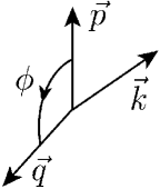
Fig. 1: Definition of azimuthal angle $\phi$ of recoil particle.

The phase volume of the final state

$$d\Gamma=(2\pi)^{-5}\frac{d^{3}k}{2\omega}\frac{d^{3}p_{1}^{\prime}}{2E_{1}^{\prime}}\frac{d^{3}p^{\prime}}{2E^{\prime}}\delta^{4}\left(p+p_{1}-p_{1}^{\prime}-p^{\prime}-k\right),$$ (4)

after introducing an auxiliary integration

$$\delta^{4}\left(p+p_{1}-p_{1}^{\prime}-p^{\prime}-k\right)=d^{4}q\delta^{4}\left(p_{1}+q-k-p_{1}^{\prime}\right)\delta^{4}\left(q-p+p^{\prime}\right),$$ (5)

can be expressed in terms of Sudakov’s variables as :

$$d\Gamma=\frac{d^{2}q\,d^{2}p\,dx}{4sx\bar{x}(2\pi)^{5}}=\frac{E^{\prime}dE^{\prime}dx\theta_{e}d\theta_{e}d\phi}{2^{7}\bar{x}\pi^{4}},$$ (6)

where $\phi=(\widehat{\vec{p},\vec{q}})$ is the azimuthal angle (see Fig. 1), delimited by two planes: the plane which contain the momenta of the initial and final electrons, ($p_{1}$,$p_{1}^{\prime}$) and the plane defined by the momenta of the initial electron and of the exchanged photon ($p_{1}$,$q$), $\theta_{e}=|\vec{p}|/(Ex)$ is the angle between initial and scattered electron directions.

In the Laboratory frame the transverse momentum $|\vec{q}|$ is related to the energy of the recoil particle. Due to four-momentum conservation the recoil proton momentum $p^{\prime}=(E^{\prime},\vec{p}{\,{}^{\prime}})$ can be written as:

$$\vec{p}{\,{}^{\prime}}^{2}=\vec{q}^{\,2}+\frac{(\vec{q}^{\,2})^{2}}{4M^{2}},$$ (7)

and the following relations hold:

$$E^{\prime\,2}=\frac{(\vec{q}^{\,2}+2M^{2}_{p})^{2}}{4M^{2}_{p}},~{}\vec{p}^{\,\,2}=(E\theta_{e}x)^{2},~{}\vec{q}^{\,\,2}=2M^{2}_{p}+2M_{p}E^{\prime}.$$ (8)

II.2 Unpolarized electron

According to the formalism developed in Ref. BFKK81 , the matrix element of the process (1) (which is illustrated in Fig. 2), for not negligible momentum transferred by the exchanged virtual photon, $|\vec{q}|$, can be written as:

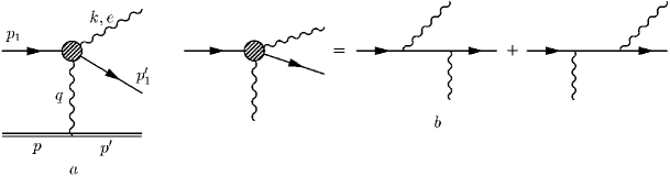
Fig. 2: Feynman diagrams which are relevant in peripheral kinematics.

$${\cal M}=\frac{(4\pi\alpha)^{\frac{3}{2}}}{\vec{q}^{\,\,2}}\frac{2}{s}\left[\bar{u}(p^{\prime})\Gamma_{\lambda}p^{\lambda}_{1}u(p)\right]\left[\bar{u}(p^{\prime}_{1})O_{\mu\nu}\tilde{p}^{\mu}e^{\nu}u(p_{1})\right],$$ (9)

where $\Gamma_{\mu}=\gamma_{\mu}$ in case of $e^{\pm}$ target, and $\Gamma_{\mu}=F_{1}(q^{2})\gamma_{\mu}+(1/4M_{p})(\hat{q}\gamma_{\mu}-\gamma_{\mu}\hat{q})F_{2}(q^{2})$ for a proton target, where $F_{1,2}(q^{2})$ are the proton form factors. The vectors $\vec{k}$, $\vec{q}$ and $\tilde{p}$ are defined in Eqs. (2).

After summing over the lepton quantum numbers, the square of the matrix element is:

$$\sum|{\cal M}|^{2}=\frac{\left(\pi\alpha\right)^{3}}{\left(\vec{q}^{\,\,2}\right)^{2}}2^{11}s^{2}D\frac{1}{4}\operatorname{Tr}\left[\hat{p}^{\prime}_{1}\left(\hat{e}\rho+\frac{\hat{e}\hat{q}\hat{\tilde{p}}}{sd_{2}}-\frac{\hat{\tilde{p}}\hat{q}\hat{e}}{sd_{1}}\right)\hat{p}_{1}\left(\rho\hat{e^{*}}+\frac{\hat{\tilde{p}}\hat{q}\hat{e^{*}}}{sd_{2}}-\frac{\hat{e^{*}}\hat{q}\hat{\tilde{p}}}{sd_{1}}\right)\right],$$ (10)

where $\rho=\frac{1}{d_{2}}-\frac{x}{d_{1}}$ and

$$D=\left\{\begin{array}[]{ll}1,&\mbox{ for~{}electron target,}\\ F_{1}^{2}(-\vec{q}^{2})+\frac{\vec{q}^{2}}{4M_{p}^{2}}F_{2}^{2}(-\vec{q}^{2})&\mbox{ for~{}proton target.}\end{array}\right.$$

In case of unpolarized final photon, the cross section can be written as:

$$M^{3}_{p}\frac{2\pi d\sigma}{dxdE^{\prime}d\vec{p}^{\,\,2}d\phi}=\frac{4\alpha^{3}}{M^{2}_{p}}DR,~{}R=\frac{M^{6}_{p}A}{(\vec{q}^{\,\,2})^{2}x\bar{x}},$$ (11)

where

$$A = (x\bar{x})^{2}\left(\frac{1}{\Delta_{1}}-\frac{1}{\Delta_{2}}\right)^{2}\left[\frac{\vec{p}^{\,\,2}}{2x}+\frac{(\vec{q}-\vec{p})(x\vec{q}-\vec{p})}{\bar{x}^{2}}\right]+$$ (12)

$$+\frac{(x\bar{x})^{2}}{\Delta_{2}}\left(\frac{1}{\Delta_{2}}-\frac{1}{\Delta_{1}}\right)\left[-\vec{p}\vec{q}-\frac{2}{\bar{x}}(x\vec{q}^{\,\,2}-\vec{p}\vec{q})\right]-$$

$$-\frac{x\bar{x}^{2}}{\Delta_{1}}\left(\frac{1}{\Delta_{2}}-\frac{1}{\Delta_{1}}\right)\left[\frac{1}{2}\vec{p}\vec{q}-\frac{2x}{\bar{x}}\vec{q}^{\,\,2}+\frac{2x}{\bar{x}}\vec{p}\vec{q}\right]+\left[\frac{(x\bar{x})^{2}}{\Delta^{2}_{2}}+\frac{(\bar{x})^{2}}{\Delta^{2}_{1}}\right]\frac{x\vec{q}^{\,\,2}}{2},$$

The quantity $R$ is calculated for $x=1/2$ and for different values of $\vec{q}^{2}$ and $\vec{p}^{2}$ in Table 1.

Introducing the photon polarization density matrix:

$$\sum_{ij}e^{\lambda}_{i}e^{*\lambda}_{j}=\frac{1}{2}[I+\xi_{1}\sigma_{1}+\xi_{3}\sigma_{3}]_{ij},$$ (13)

Eq. (10) can be written in the form

$$\sum|{\cal M}|^{2}\sim A+B\xi_{1}+C\xi_{3}=A[1+X_{1}\xi_{1}+X_{3}\xi_{3}].$$

The polarization state of bremsstrahlung photon is characterized by the Stokes parameters, which have the form Akhiezer

$$X_{1}=\frac{B}{A},\quad X_{3}=\frac{C}{A}.$$ (14)

with $B$ and $C$ given by:

$$B = (x\bar{x})^{2}\left(\frac{1}{\Delta_{2}}-\frac{1}{\Delta_{1}}\right)^{2}\left[x\vec{q}^{\,\,2}\sin(2\phi)-(1+x)|\vec{p}||\vec{q}|\sin(\phi)\right]+$$ (15)

$$+\frac{(x\bar{x})^{2}}{\Delta_{2}}\left(\frac{1}{\Delta_{2}}-\frac{1}{\Delta_{1}}\right)\left[x\vec{q}^{\,\,2}\sin(2\phi)-|\vec{p}||\vec{q}|\sin(\phi)\right]+$$

$$+\frac{2x^{2}\bar{x}}{\Delta_{1}}\left(\frac{1}{\Delta_{2}}-\frac{1}{\Delta_{1}}\right)\left[\vec{q}^{\,\,2}\sin(2\phi)-|\vec{p}||\vec{q}|\sin(\phi)\right],$$

$$C = x^{2}\left(\frac{1}{\Delta_{2}}-\frac{1}{\Delta_{1}}\right)^{2}\left[\vec{p}^{\,\,2}+x\vec{q}^{\,\,2}\cos(2\phi)-2x|\vec{p}||\vec{q}|\cos(\phi)\right]-$$ (16)

$$-\frac{2x^{2}\bar{x}}{\Delta_{2}}\left(\frac{1}{\Delta_{2}}-\frac{1}{\Delta_{1}}\right)\left[x\vec{q}^{\,\,2}\cos(2\phi)-|\vec{p}||\vec{q}|\cos(\phi)\right]+$$

$$+\frac{2x^{2}\bar{x}}{\Delta_{1}}\left(\frac{1}{\Delta_{2}}-\frac{1}{\Delta_{1}}\right)\left[\vec{q}^{\,\,2}\cos(2\phi)-|\vec{p}||\vec{q}|\cos(\phi)\right]-\frac{(x\bar{x})^{2}}{\Delta_{1}\Delta_{2}}\vec{q}^{\,\,2}\cos(2\phi),$$

where $\Delta_{1,2}$ are defined in Eqs.(3a,3b).

The quantities $X_{1}$ and $X_{3}$ are calculated in Tables 2 and 3 for typical kinematics. As one can see, the values of $X_{1}$ are quite constant and very large, of the order of 80%. The values of $X_{3}$ are also sizeable and increase with energy. The magnitude of the cross section can be calculated from Eq. (11) and Table 2 , the kinematical coefficient $4\alpha^{3}/M_{p}^{2}$ being of the order of 700 pb. So the bremsstrahlung with unpolarized initial electron can be used as a polarimeter one. Really it has large cross section and the characteristics of linear polarization of photon depends smoothly in known way on kinematic

$\vec{q}^{\,2}$, GeV / $\vec{p}^{\,2}$, GeV	0.50	1.00	1.50	2.00	2.50	3.00
0.50	1.583	0.489	0.225	0.127	0.080	0.055
1.00	0.493	0.198	0.102	0.061	0.040	0.028
1.50	0.217	0.104	0.059	0.037	0.025	0.018
2.00	0.114	0.062	0.037	0.025	0.017	0.013
2.50	0.067	0.040	0.026	0.018	0.013	0.010
3.00	0.043	0.027	0.018	0.013	0.010	0.007

Table 1: calculated values for the term $R$ (Eq. (11)) for $\phi=\pi/2$, $x=1/2$ as a function of $\vec{q}^{\,2}$ and $\vec{p}^{\,2}$.

$\vec{q}^{\,2}$, GeV / $\vec{p}^{\,2}$, GeV	0.50	1.00	1.50	2.00	2.50	3.00
0.50	-0.841	-0.853	-0.845	-0.827	-0.806	-0.785
1.00	-0.816	-0.841	-0.851	-0.853	-0.851	-0.845
1.50	-0.799	-0.827	-0.841	-0.849	-0.853	-0.853
2.00	-0.784	-0.816	-0.831	-0.841	-0.847	-0.851
2.50	-0.769	-0.807	-0.823	-0.833	-0.841	-0.846
3.00	-0.754	-0.799	-0.816	-0.827	-0.834	-0.841

Table 2: The Stokes parameter $X_{1}$ (Eq. (14)) for $\phi=\pi/2$, $x=1/2$ as a function of $\vec{q}^{\,2}$ and $\vec{p}^{\,2}$.

$\vec{q}^{\,2}$, GeV / $\vec{p}^{\,2}$, GeV	0.50	1.00	1.50	2.00	2.50	3.00
0.50	0.397	0.483	0.534	0.569	0.596	0.617
1.00	0.308	0.397	0.447	0.483	0.511	0.534
1.50	0.251	0.345	0.397	0.432	0.460	0.483
2.00	0.209	0.308	0.360	0.397	0.424	0.447
2.50	0.175	0.277	0.332	0.369	0.397	0.419
3.00	0.147	0.251	0.308	0.345	0.374	0.397

Table 3: The Stokes parameter $X_{3}$ (Eq. (14)) for $\phi=\pi/2$, $x=1/2$ as a function of $\vec{q}^{\,2}$ and $\vec{p}^{\,2}$.

II.3 Circular photon polarization

The longitudinal polarization of the initial electron induces a circular polarization of the photon BGGK04 :

$$X_{2}=\frac{|{\cal M}_{+}|^{2}-|{\cal M}_{-}|^{2}}{|{\cal M}_{+}|^{2}+|{\cal M}_{-}|^{2}},$$ (17)

where ${\cal M}_{\pm}$ is the light-cone projection of matrix element of the subprocess of creation of a photon with chirality $\pm$ in the process where the lepton has positive chirality : $e(p_{1},+)+\gamma^{*}\to\vec{e}(p^{\prime}_{1},+)+\gamma(k,\pm)$.

Fig. 3: The Stokes parameter $X_{2}$ as a function of the energy fraction carried by the photon $\bar{x}$.

The Stokes parameter $X_{2}$, related to the circular polarization of the photon depends only on the energy fraction carried by the photon:

$$X_{2}=\frac{1-x^{2}}{1+x^{2}}=\frac{\bar{x}(2-\bar{x})}{2-2\bar{x}+\bar{x}^{2}}.$$ (18)

One can see that the larger is the energy of the photon, the larger is the degree of polarization (Fig. 3).

Conclusion

We calculated the linear polarization of the bremsstrahlung photon for unpolarized high-energy $e-p$, $e-e^{\pm}$ scattering at small scattering angles and high energy. The relevant Stokes parameters are functions of kinematical variables such as the transferred momentum, the polar and azymuthal angles of the photon and its energy fraction. For the case of longitudinally polarized initial electrons, the photon has nonzero circular polarization which depends only on its energy fraction.

The accuracy of formulae given above is determined by radiative corrections and on the omitted terms. We estimate it as

$$1+O\left(\frac{\vec{p}^{\,2}}{s},\frac{\alpha}{\pi}\ln\frac{\vec{p}^{\,2}}{m^{2}},\frac{m^{2}}{\vec{p}^{\,2}}\right).$$ (19)

As an example, for the upgraded JLab facility ($E\approx 12~{}\mbox{GeV}$) it is of order $\sim~{}10\%$.

In this paper we emphasized the possibility to obtain polarized photons in the process of peripheral scattering of leptons. We derived the expressions that relate the polarization parameters and the cross section to the relevant kinematical variables and calculated these observables, for different kinematical conditions.

We showed that the cross section and the degree of polarization is sufficiently large and that this process should be taken into consideration for designing photon polarimeters in the GeV range.

It should be stressed that the Stokes parameters that characterize the bremsstrahlung photon polarization do not depend neither on the initial energy nor on the target mass.

References

- (1) U.Fano Phys. Rev. 93, 121 (1954); M. P. Rekalo and I. M. Sitnik, Phys. Lett. B 356, 434 (1995).
- (2) M. Porrmann, Nucl. Phys. A 399 (1983) 365.
- (3) V. F. Boldyshev, E. A. Vinokurov, N. P. Merenkov and Yu. P. Peresunko, Phys. Part. Nucl. 25 (1994) 292 and Refs. therein.
- (4) K. Kondo et al., Nucl. Instrum. Meth. 114, 365 (1974).
- (5) E. Bartos, M. V. Galynskii, S. R. Gevorkyan and E. A. Kuraev, Nucl. Phys. B 676, 390 (2004).
- (6) V. N. Baier, E. A. Kuraev, V. S. Fadin and V. A. Khoze, Phys. Rept. 78, 293 (1981).
- (7) A.I. Akhiezer, V.B. Berestetskii, Quantum Electrodynamics (1981)