Sagnac Rotational Phase Shifts in a Mesoscopic Electron Interferometer with Spin-Orbit Interactions

Abstract

The Sagnac effect is an important phase coherent effect in optical and atom interferometers where rotations of the interferometer with respect to an inertial reference frame result in a shift in the interference pattern proportional to the rotation rate. Here we analyze for the first time the Sagnac effect in a mesoscopic semiconductor electron interferometer. We include in our analysis Rashba spin-orbit interactions in the ring. Our results indicate that spin-orbit interactions increase the rotation induced phase shift. We discuss the potential experimental observability of the Sagnac phase shift in such mesoscopic systems.

I Introduction

In the last decade experimental developments in mesoscopic condensed matter and AMO (atomic, molecular, and optical) physics, such as the explosive growth in semiconductor nanostructures, the creation of atomic Bose-Einstein condensates (BEC) and ultra-cold atom interferometers, and the interest in quantum computation and information, have caused phase coherence and related phenomena to receive extraordinary attention. Particularly interesting are quantum interference phenomena in ballistic transport through high mobility nanostructures in which electron propagation is described by quantum mechanics rather than by classical transport. This has lead to novel experiments with matter wave interferometers (MI’s) for electrons electron-interferometers and quantum dot structures quantum-dots demonstrating quantum interference between different paths.

Matter wave interferometry is a key paradigm for quantum interference and dates back to the early electron-diffraction experiments. Recent advances show considerable promise for the development of new devices, mostly because the sensitivity of MI’s Clauser ; Berman far exceeds that of their optical counterparts for many important applications. Although both optical interferometers and MI’s are able to detect rotations due to the Sagnac effect, the sensitivity of atom-interferometer (AI) based rotation sensors, however, can be as much as $Mc^{2}/\hbar\omega\sim 10^{10}$ times greater Clauser ; Scully than that of optical ones Chow . (Here $M$ is the atomic mass and $\hbar\omega$ is the energy of a photon.) Current generation laboratory AI’s Gustavson already outperform commercially available ring laser gyroscopes Chow . Optical gyroscopes are now used on virtually all commercial aircraft as well as on spacecraft for inertial navigation. The potential improvement for rotation sensing with AI’s, along with their ability to accurately detect small changes in gravitational fields, has resulted in intense activity within the AMO community to develop AI sensors for inertial navigation, geophysical prospecting, and tests of general relativity Gustavson ; McGuirk ; Durfee .

In 1913, Sagnac demonstrated that it is possible to detect rotations with respect to an inertial frame of reference with an interferometer, using the rotation-induced path length difference between its two arms. The phase shift is easily understood if one considers a ring shaped Mach-Zehnder interferometer of radius $R$ rotating about its axis at the rate $\Omega$. In one arm of the interferometer, the particles are co-propagating with the rotation, which increases the distance particles have to travel before exiting by $\approx R\Omega t$. For the other arm, particles are moving opposite to the direction of rotation and the distance they must travel before exiting is decreased by the same amount. As a result, there is a path length difference proportional to $\Omega$.

It should in principle be possible to observe this effect in another type of matter wave device - electron interferometers (EI’s). Mesoscopic semiconductor EI’s have been predominantly used for studying transport and quantum interference in low dimensional systems electron-interferometers . Recently there has been a number of papers on their use to control and generate spin currents in the presence of spin-orbit(SO) coupling Junsaku ; Konig ; Frustaglia ; shelykh ; BranislavNikolic . Surprisingly, there has been no discussion of using them as gyroscopes. To date, the only experiments on the rotation induced Sagnac effect for electrons were done with electron beams in vacuum Hasselbach . In comparison to optical or atom interferometers, EI’s are much smaller, can be integrated with other solid state devices, and are in many ways more robust due to the monolithic solid state structure.

The practical importance of the Sagnac effect for navigation combined with the technological advantages of solid state devices, raises the question as to how easily this effect could be exploited in solid state EI’s. For electrons with effective mass $m^{*}\approx 0.1m_{e}$, the enhancement factor relative to an optical interferometer with equal area is $m^{*}c^{2}/\hbar\omega\sim 10^{5}-10^{6}$. On the other hand, the main disadvantage of electron interferometers is the phase coherence length ${L_{\Phi}}\approx l_{mfp}$, which for electrons in solids limits the area of an interferometer to approximately ${L_{\Phi}}^{2}/\pi$. Since the rotational phase shift is proportional to the enclosed area, this limitation implies a phase shift several orders of magnitude smaller than for current AI’s Gustavson ; Durfee . At the same time we note that each order of magnitude improvement in the mean free path $l_{mfp}$, resulting from improved fabrication techniques, yields a hundred-fold increase in the maximum area, and as a consequence, in the rotational phase shift. It is worth mentioning, however, that recently several papers have pointed out that the rotation induced Sagnac effect could be observed in arrays of coupled optical microring waveguides by using ’slow’ light peng ; Scheuer . The radii of the microrings is $\sim 10\mu m$, which is only about one order of magnitude larger than already demonstrated semiconductor rings for electrons and holes Konig ; morpurgo ; yau . Recently, the Sagnac effect has been observed in the electronic conductance of carbon nanotube loops with diameters $\sim 1\mu m$ although the origin of the Sagnac phase difference was not due to an externally applied rotation of the loops refael .

The main goal of this paper is to investigate a way to enhance the Sagnac phase shift to readily detectable values. To this end, we analyze the coherent interplay of the Sagnac effect and Rashba spin-orbit interaction and estimate the resulting enhancement of the Sagnac phase shift. Indeed, we find that the interplay between the spin interference driven by the spin-orbit interaction and the Sagnac effect result in a larger phase shift for a given rotation rate. This increase in the phase shift can be interpreted as a larger effective area for the interferometer.

The paper is organized as follows: Section II establishes the model and introduces the slowly varying envelope approximation as a mathematical technique for solving the Schrödinger equation in the ring. To justify the applicability of the SVE, we compare our results to exact numerical solutions of the Schrödinger equation for several parameter values. In Sec. III we present the results of our simulations, and calculate the enhancement of rotational phase shifts. We also discuss the effect of quantum noise on the detectability of rotational phase shifts. Finally, Sec. IV is a summary and outlook where we discuss how to optimize the phase shift by integrating a series of EI’s into an array.

II Theoretical Model

We consider a quasi-one-dimensional ring of radius $r_{0}$, which could be defined in a two-dimensional electron Konig ; morpurgo or hole yau semiconductor heterostructure [Fig. 1(a)]. We presume that the arms of the ring behave as a ballistic conductor (i.e. the length of the arms is smaller then the electron mean free path). The ring is coupled to two electron reservoirs with a bias voltage $V_{1}-V_{2}$ resulting in a current $I=G(V_{1}-V_{2})$. In the growth direction (z-axis), which is perpendicular to the plane of the ring, a static magnetic field ${\bf B}=\nabla\times{\bf A}$ and electric field ${\bf E}$ are applied. The electric field comes from the electrostatic potential of a biased gate above the plane of the ring and has no contribution from the static vector potential ${\bf A}$. Due to the applied magnetic field B, there is a nonzero Zeeman splitting between electron spin states as well as a finite magnetic flux through the ring that would give rise to Aharonov-Bohm oscillations.

In semiconductor heterostructures with structure inversion asymmetry, such as InGaAs/InAlAs Nitta2 or HgTe/HgCdTe Konig quantum wells, the dominant spin-orbit interaction is given by the Rashba Hamiltonian Rashba ,

$$H_{int}=\alpha{\bf{\sigma}}\cdot{\bf E}\times\Pi=\alpha_{R}\hat{z}\cdot({\bf\sigma}\times{\Pi})$$ (1)

where $\sigma$ is the vector of the Pauli spin operators, $\Pi={\bf p}-e{\bf A}$ the electron momentum, and ${\alpha_{R}}=\alpha E_{z}$ the Rashba constant. For electrons traveling around the ring, E gives rise to a momentum dependent magnetic field ${\bf B}_{R}$ in the plane of the ring due to the SO coupling of the electron spin with its center-of-mass motion. An important feature of the Rashba interaction is that the strength of the SO interaction is proportional to the external electric field, which enables easy control by the gate above the ring. The spins precess around ${\bf B}_{eff}={\bf B}+{\bf B}_{R}$ [Fig. 1(b)] as they propagate around the ring. This leads to interference between the spin directions of an electron whose wave function is coherently split between the two paths of the interferometer and then later coherently recombined upon exiting. Note that because we consider only ballistic transport here, the Rashba term only gives rise to coherent coupling between the spin states and does not cause dephasing of the spin coherence due to scattering of the orbital wave function.

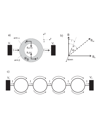
Figure 1: (a) Schematic diagram of an electron interferometer: 1D ring of radius $r_{0}$ subject to Rashba spin-orbit coupling and in the presence of an external magnetic field ${\bf B}$. (b) Effective magnetic, ${\bf B}_{eff}={\bf B}+{\bf B}_{r}$ field that spins perceive while traveling around the ring. (c) A one dimensional array of ring interferometers in series.

The effective 1D Hamiltonian for electrons (charge $e<0$ and effective mass $m^{*}$) propagating in ring subject to Zeeman and Rashba coupling, with coupling constants $\mu$ and $\alpha_{R}$, respectively, is Frustaglia ; Meijer ,

$$\hat{H}_{1D}(\varphi)=\frac{\hbar\omega_{0}}{2}(-i\frac{\partial}{\partial\varphi}+\frac{\Phi}{\Phi_{0}})^{2}+\frac{\hbar\omega_{B}}{2}\sigma_{Z}$$

$$+\frac{\hbar\omega_{R}}{2}(\cos\varphi\sigma_{x}+\sin\varphi\sigma_{y})(-i\frac{\partial}{\partial\varphi}+\frac{\Phi}{\Phi_{0}})$$

$$-i\frac{\hbar\omega_{R}}{4}(\cos\varphi\sigma_{y}-\sin\varphi\sigma_{x})$$ (2)

where the frequencies $\omega_{0}=\hbar/(m^{*}r_{0}^{2})$, $\omega_{B}=2\mu B/\hbar$, and $\omega_{R}=2\alpha_{R}/\hbar r_{0}$, $\Phi=\pi r_{0}^{2}B$, and the flux quantum $\Phi_{0}=h/e$ have been introduced. Here we have made use of the form of the vector potential for a uniform B-field in the z-direction, ${\bf A}={\bf\hat{e}}_{\varphi}rB/2$, to reexpress all quantities involving ${\bf A}$ in terms of the magnetic flux through the ring.

If the ring is rotating with angular velocity $\Omega$ about the axis perpendicular to the ring, the effective distance that particles have to travel before exiting the ring is increased by $\delta l_{\alpha}={r_{0}}\Omega t_{\alpha}$ for particles co-propagating with the rotation and decreased by the amount $\delta l_{\beta}={r_{0}}\Omega t_{\beta}$ for particles that are moving in the opposite direction. Here we assume that particles going from left to right in the upper arm ($\alpha$) in Fig. 1(a) are co-propagating with the rotation while those going in the same direction through the lower arm ($\beta$) are counter-propagating. For small $\Omega$ such that $\delta l_{\alpha(\beta)}\ll l_{\alpha(\beta)}$ where $l_{\alpha(\beta)}$ is the path length of the upper co-propagating (lower counter-propagating) arm, then $t_{\alpha(\beta)}=(l_{\alpha(\beta)}\pm\delta l_{\alpha(\beta)})/v\approx\l_{\alpha(\beta)}/v=\pi{r_{0}}/v$ where $v$ is the velocity of the particles. This causes a Sagnac phase difference between two counter-propagating de Broglie waves in the ring of $\Delta\phi=k[(l_{\alpha}+\delta l_{\alpha})-(l_{\beta}-\delta l_{\beta})]=k2\pi{{r_{0}}^{2}}\Omega/v=2A\Omega m^{*}/\hbar$, where $k=m^{*}v/\hbar$ is the wave number of an electron, $A={{r_{0}}^{2}}\pi$ is the area enclosed by the arms of the interferometerScully . This derivation of the Sagnac phase shift assumes that the spin of the particle is not affected by the rotation. However, in addition to the normal Sagnac phase shift, the rotation of the ring changes the distance that the spins precess around ${\bf B}_{eff}$ as they propagate along the two arms. The relative orientations of the spins from the two arms when recombined has now been changed as a result of the rotation. The resulting spin interference will give a contribution to the Sagnac phase shift, $\Delta\phi$, that is a function of $\Omega$ and $|{\bf B}_{eff}|$.

When the ring is rotating, the system could be described by the same Hamiltonian as the one given in Eq. (2), but the point where the two counter-propagating electron waves recombine and interfere would change its position with time. An easier way to analyze interference in a rotating ring is to change the reference system in which we observe the process from the non-rotating to the rotating one. In the rotating frame of reference, the angular momentum of particles co-propagating with the rotation is decreased while those that are counter-propagating is increased, similar to the Doppler effect. The wave functions in the two reference frames are related by $\Psi_{R}=\hat{R}\Psi$, where $\Psi_{R}$ and $\Psi$ are the wave functions in the rotating and non-rotating frames, respectively, and $\hat{R}=\exp[i\Omega t\hat{n}\cdot\vec{L}/\hbar]$ is the rotation operator ($\hat{n}$ is the rotation axis and $\vec{L}$ the angular momentum operator). Only rotations around the axis perpendicular to the plane of the ring will result in a relative phase shift between the two arms. For this reason we set $\vec{L}\rightarrow L_{z}$ without loss of generality. The Hamiltonian for an electron in the rotated frame is then given by:

$$\hat{H}_{R}(\varphi)=\hat{H}_{1D}(\varphi)+i\hbar\Omega\frac{\partial}{\partial\varphi}$$ (3)

The energy eigenfunctions can be expressed in the following form:

$$\Psi_{R}(\varphi,t)=e^{-\frac{iE}{\hbar}t}\Psi_{R}(\varphi)=e^{-\frac{iE}{\hbar}t}\left[\begin{array}[]{ccc}S_{\uparrow}(\varphi)\\ S_{\downarrow}(\varphi)\end{array}\right]e^{iKr_{0}\varphi}$$ (4)

where $S_{\uparrow},S_{\downarrow}$ are the angular dependent spinors for spin states oriented along the z-axis with energy $E$ and momentum $K$ propagating inside the ring with radius $r_{0}$. This is inserted into the time-dependent Schrödinger equation for the Hamiltonian in Eq. (3), giving us a system of second order differential equations for the envelope function $S_{\uparrow},S_{\downarrow}$. If the envelopes functions are smooth functions that vary much slower than the carrier wave,

$$|\partial S_{\sigma}(\varphi)/\partial\varphi|\ll Kr_{0}|S_{\sigma}(\varphi)|,$$

we can neglect the second order derivatives. This is known as the slowly varying envelope (SVE) approximation in optics Meystre . While SVE is a widely used technique in nonlinear and atom optics, it is not common in mesoscopic transport. With this approximation the system becomes,

$$\left[\begin{array}[]{ccc}\dot{S_{\uparrow}}\\ \dot{S_{\downarrow}}\end{array}\right]=M\left[\begin{array}[]{ccc}i\left(aP_{1}-\left(\frac{\omega_{R}}{\omega_{0}}\right)^{2}(b+1)\right)&i(ab-P_{2})\frac{\omega_{R}}{\omega_{0}}e^{-i\varphi}\\ i(a(b+1)-P_{1})\frac{\omega_{R}}{\omega_{0}}e^{i\varphi}&i\left(aP_{2}-\left(\frac{\omega_{R}}{\omega_{0}}\right)^{2}b\right)\end{array}\right]\left[\begin{array}[]{ccc}S_{\uparrow}\\ S_{\downarrow}\end{array}\right]$$ (5)

where dots over $S_{\uparrow},S_{\downarrow}$ denote derivatives with respect to the angular position in the ring $\varphi$, and

$$M=\left(\left(\frac{\omega_{R}}{\omega_{0}}\right)^{2}-a^{2}\right)^{-1},\qquad\quad$$

$$a=2\left(Kr_{0}+\frac{\Phi}{\Phi_{0}}-\frac{\omega}{\omega_{0}}\right),b=Kr_{0}+\frac{\Phi}{\Phi_{0}}-\frac{1}{2},$$

$$P_{1/2}=\left[2\frac{2E}{\hbar\omega_{0}}+\left(Kr_{0}+\frac{\Phi}{\Phi_{0}}\right)^{2}-2Kr_{0}\frac{\omega}{\omega_{0}}\pm\frac{\omega_{B}}{\omega_{0}}\right]$$

These coupled first order differential equations are numerically easier to integrate than the second order coupled equations for $S_{\sigma}$ that would be directly obtained from the Schrodinger equation.

In the Landauer-Buttiker formalism, the zero-temperature conductance of a ballistic conductor is given by:

$$G=\sum_{\sigma^{\prime},\sigma}G^{\sigma^{\prime}\sigma}=\frac{e^{2}}{h}\sum_{\sigma^{\prime},\sigma}\sum_{m^{\prime},m=1}^{M}T_{m^{\prime}m}^{\sigma^{\prime}\sigma}$$ (6)

where $T_{m^{\prime}m}^{\sigma^{\prime}\sigma}$ denotes the quantum mechanical probability of transmission between incoming $(m,\sigma)$ and outgoing $(m^{\prime},\sigma^{\prime})$ asymptotic states. The labels $m,m^{\prime}$ and $\sigma,\sigma^{\prime}$ refer to the corresponding orbital mode and spin quantum numbers, respectively. From Eq. (6) it can be seen how a change of the transmission coefficients due to interference from rotation induced phase shifts causes a modulation of the current through the ring. For convenience, we will restrict our discussion to a single orbital mode and drop the subscripts for the transmission probabilities.

By specifying the spin states of the electrons when they enter the ring, $S_{\sigma,\alpha(\beta)}(0)$, we can obtain $S_{\sigma^{\prime},\alpha(\beta)}(\pm\pi)$ at the end points of the interferometer arm where the wave function is recombined. From this the transmission coefficients, $T^{\sigma^{\prime}\sigma}$, and hence the conductance can be directly calculated. For example, if spin up polarized current enters the ring and the wave functions is equally split between the two arms, $S_{\uparrow,\alpha}(0)=S_{\uparrow,\beta}(0)=1/\sqrt{2}$, then the probability of measuring a spin down electron leaving the ring on the other side is then $T^{\downarrow,\uparrow}=|S_{\downarrow,\alpha}(\pi)+S_{\downarrow,\beta}(-\pi)|^{2}/4$.

If the leads connected to the ring are unpolarized, i.e. the leads are an incoherent mixture of spin-up and down, then it is only the total charge conductance that will be measured. On the other hand, the field of spintronics has been making rapid progress towards methods for generating and measuring spin polarized currents by such methods as ferromagnetic leads and the spin hall effect zutic ; awschalom ; tinkham . One can then imagine that incident on the ring from the left lead is a current that is spin polarized along the z-direction and that in the second lead one can measure the spin polarization of the current exiting the ring. In this case, one is directly measuring the spin polarized conductances, $G^{\sigma^{\prime}\sigma}$. In the next section we consider both scenarios.

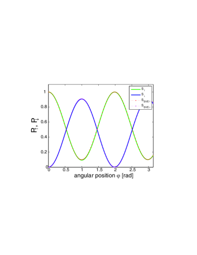
Figure 2: Comparison between SVE and numerical solution of Schrodinger equation without SVE: Probabilities for spin up ($P_{\uparrow}=|S_{\uparrow}(\varphi)|^{2}$) and spin down ($P_{\downarrow}=|S_{\downarrow}(\varphi)|^{2}$) states, along one arm of interferometer assuming spin-down electrons enter that arm. Here $r_{0}=1000nm$, $Q_{R}=3$, and there is no external magnetic field.

III Results

In our simulation of the electron interferometer we used $r_{0}=1000nm$ for the radius of ring and for the electron we chose an effective mass $m^{*}=0.067m_{0}$ and wave number $K=0.1nm^{-1}$. In addition to this we focus on ${\bf B}=0$ from here on since this is expected to produce the maximal spin interference between the two arms. We solved Eq. (5) numerically using the SVE approximation, and in order to check its validity we did the same calculation including the second order derivatives. The comparison between the two methods is shown in Fig.2, where we see that the difference between results derived without the approximation (solid line) and with the SVE approximation (dashed line) is negligibly small. The SVE approximation is justified only when $1/K$ is much less than the distance over which the envelope functions change significantly, which is given by the spin precession length, $\ell_{SO}=\hbar\pi/\alpha_{R}m^{*}$. In terms of $\alpha_{R}$ and $K$ this condition is then,

$$\frac{\hbar\pi K}{\alpha_{R}m^{*}}\gg 1$$

Application of this mathematical technique in the future can considerably reduce calculation time needed for more complex problems. In particular, it provides an alternative to other techniques currently used such as numerical evaluation of real space Greens functions BranislavNikolic .

The spatial Rabi oscillations between spin states in Fig. 2 are not of full amplitude. This is because the diagonal terms in Eq. 5 are not the same, which means that the slowly varying envelope functions are not degenerate. It is well known from the theory of two-level quantum systems that the amplitude of the oscillations between states decreases with increasing energy difference between the states. How this ’energy difference’ arises from the underlying Hamiltonian Eq. 2 can be understood by noting that to obtain Eq. 5 for the stationary states in an arm of the ring, we have expressed the spatial equations of motion in the form

$$i\hbar\frac{\partial}{\partial\varphi}\Psi=\tilde{H}\Psi.$$

This has the form of a Scrodinger equation but with the substitution $t\rightarrow\varphi$. To obtain this form from Eq. 2 one must multiply both sides by $[\frac{\hbar\omega_{R}}{2}(\cos\varphi\sigma_{x}+\sin\varphi\sigma_{y})]^{-1}$, which gives rise to terms proportional to $\sigma_{z}$.

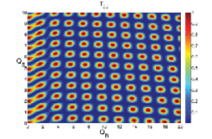
Figure 3: Spin polarized transmission coefficient, $T^{\downarrow,\downarrow}$, for an electron propagating through EI for $B=0$, for different values of Rashba SO coupling strength ($Q_{R}=\omega_{R}/\omega_{0}$) and Sagnac strength ($Q_{S}=\Omega/\omega_{0}$). This is the probability that an electron with spin down at the entrance of the ring has the same spin when it exits the ring

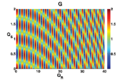
Figure 4: Total conductance in units of $e^{2}/h$ for an electron propagating through EI for $B=0$ and different values of Rashba SO coupling strength ($Q_{R}=\omega_{R}/\omega_{0}$) and Sagnac strength ($Q_{S}=\Omega/\omega_{0}$).

Having found values for $S_{\uparrow}$ and $S_{\downarrow}$ we determined the transmission coefficients for different magnitudes of Rashba SO coupling and rotation rates. Figures 3 and 4 shows $G^{\downarrow,\downarrow}$, assuming a spin down polarized current incident on the ring, as well as the total conductance, $G$, for unpolarized currents in units of $e^{2}/h$, respectively. One can conclude from both figures that the Rashba and Sagnac effect do not give rise to separate contributions to the transmission phase since the interference pattern does not lie along horizontal or vertical lines.

Let us focus on Fig. 3, which involves only a single transmission probability that can be written in the form $T^{\sigma,\sigma}\propto\cos^{2}(\Delta\phi)$. Now let us assume that the phase shift can be written as $\Delta\phi=f(Q_{S})+g(Q_{R})$ where $f(Q_{S})$ and $g(Q_{R})$ are some functions of the dimensionless rotations rate, $Q_{S}=\Omega/\omega_{0}$, and the dimensionless Rashba term $Q_{R}=\omega_{R}/\omega_{0}$. In this case one can see that if $Q_{R}(Q_{S})$ is fixed and $Q_{S}(Q_{R})$ allowed to vary, which corresponds to moving along a vertical (horizontal) line in Fig. 3, then the minima and maxima of the interference pattern should lie entirely along the vertical (horizontal) line. As one can see, however, the minima and maxima of the interference pattern follow lines that deviate from vertical and horizontal. This indicates that the phase of $T^{\sigma,\sigma}$ is a nonlinear combination of $Q_{R}$ and $Q_{S}$.

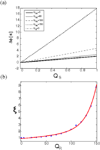
Figure 5: (a) Sagnac rotational phase shift as a function of the rotation rate $Q_{S}=\Omega/\omega_{0}$ for different values of the Rashba SO interaction strength, $Q_{R}$. Phase shift, $\Delta\phi$ is in units of $\pi$ radians (b) Dimensionless enhancement factor, $\xi$, as a function of $Q_{R}$. Dots are slopes of the curves in (a) as well as for other values of $Q_{R}$ not shown in (a). The solid line is a numerical fit to the points.

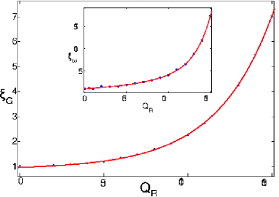
Figure 6: Dimensionless enhancement factor for the total conductance, $\xi_{G}=\left[\partial G(Q_{R},Q_{S})/\partial Q_{S}\right]_{max}/\left[\partial G(Q_{R}=0,Q_{S})/\partial Q_{S}\right]_{max}$, as a function of $Q_{R}$. Dots are numerically calculated values of $\xi_{G}$ for different $Q_{R}$ The solid line is a numerical fit to the points. Inset, $\xi_{\omega}(Q_{R})=T(Q_{R}=0)/T(Q_{R})$ is the frequency of the oscillations in $G$ as a function of $Q_{S}$ for different $Q_{R}$. Here, $T(Q_{R})$ is the period of the oscillations in $G$ for fixed $Q_{R}$ as $Q_{S}$ is increased.

In the case of spin polarized transport, the rotational phase shift $\Delta\phi$ can be uniquely equated with the phase of the interference pattern in Fig. 3 since it results from only a single transmission probability. In Fig. 5 we have extracted $\Delta\phi$ as a function of $\Omega$ for different values of $Q_{R}$ from our numerical results for $T^{\downarrow,\downarrow}$. The Sagnac phase shift with no Rashba effect is given by the dash-dotted line, which is indistinguishable from the line for $Q_{R}\!\!=\!\!5$ (thick solid line). This confirms that for weak SO coupling ($Q_{R}\lesssim 10$) there is only negligible mixing between the SO coupling and the rotational phase shift. For higher values of $Q_{R}$, the mixing becomes stronger, which is manifested by a steeper slope. Our numerical results indicate that the rotation induced phase shift is approximately

$$\Delta\phi\cong\xi 2\pi r_{0}^{2}\Omega m^{*}/\hbar$$ (7)

where $\xi\geq 1$ is an enhancement factor due to the SO coupling, which is shown in Fig. 5(b), and for which a numerical fit yields,

$$\xi(Q_{R})\approx 0.9\exp(0.007Q_{R})+0.003\exp(0.05Q_{R})$$

By increasing $Q_{R}$, it is possible to more easily detect small changes in the angular velocity.

By contrast, the total conductance involves a summation of four transmission probabilities that do not necessarily oscillate in phase with each other. In this case it is harder to define the rotation induced phase shift. However, the quantity that is of most interest experimentally is how much the conductance changes due to a small change in $Q_{S}$, $\Delta G\approx\left(\partial G/\partial Q_{S}\right)\Delta Q_{S}$. This allows us to define an enhancement, $\xi_{G}$,

$$\xi_{G}(Q_{R})=\frac{\left[\partial G(Q_{R},Q_{S})/\partial Q_{S}\right]_{max}}{\left[\partial G(Q_{R}=0,Q_{S})/\partial Q_{S}\right]_{max}}$$ (8)

where $max$ means the maximum magnitude of the slope for fixed $Q_{R}$. It is worth noting that if we assume a simple interference pattern of the form $G=A\cos^{2}[\Delta\phi]$ and use $\Delta\phi$ in Eq. 7, then we obtain from Eq. 8 $\xi_{G}=\xi$, which shows that Eq. 8 is consistent with our definition of $\xi$ for the spin polarized case. Fig. 6 shows $\xi_{G}$ as a function of $Q_{R}$. As one can see, $\xi_{G}\sim\xi$ for all $Q_{R}$. Thus the enhancement can just as easily be seen in the total conductance. Finally, the inset of Fig. 6 shows the oscillation frequency for the interference pattern in $G$ for different values of $Q_{R}$ (moving along vertical lines in Fig. 4). As one can see, the oscillation frequency increases more rapidly than $\xi_{G}$. This is because the amplitude of the oscillations decrease at a rate that is smaller than the rate of increase in the frequency. As a result $\xi_{G}$ increases but more slowly than the oscillation frequency.

The enhancement factors, $\xi$ and $\xi_{G}$, are a result of the different spin orientations of electrons created in the two arms. The spin of electrons going through the upper arm precess around ${\bf B}_{eff}$ by a larger angle before exiting as compared to the lower arm. This is due to the longer path length of the upper arm. As a result, the orientations of the spins from the upper and lower arms are different when recombined at the second lead and this imbalance in the spin precession angles changes the spin resolved conductances. Recently it was demonstrated Gvozdic that by using holes instead of electrons it is possible to increase the strength of the Rashba interaction by about three orders of magnitude. Based on the results presented here, such extremely large Rashba strengths ($Q_{R}\sim 1000-10000$) should lead to Sagnac phase shifts that are orders of magnitude larger than shown here. However, for such large $Q_{R}$ the SVE approximation breaks down and new numerical techniques must be sought.

The minimum detectable phase difference in matter wave interferometers, $\Delta\varphi_{min}$, is determined by the quantum fluctuations in the measured phase difference. These fluctuations are the result of the partition noise (also referred to as shot noise) that results from the splitting and recombining of the particles at the beam splitters. For uncorrelated particles the noise is Poissonian and the minimum detectable phase shift is Scully

$$|\Delta\varphi_{min}|=\frac{1}{\sqrt{N}}$$ (9)

where $N$ is the total number of particles that pass through the interferometer during the measurement time. This result ignores quantum statistics. If quantum statistics are accounted for, it is found that $|\Delta\varphi_{min}|$ continues to scale like $N^{-1/2}$ for bosons and fermions search-meystre . The number of electrons passing through the ring per unit time is proportional to the current through the ring $I$. By equating the rotational phase shift with the shot-noise limited minimum detectable shift, $|\Delta\phi|=|\Delta\varphi_{min}|$ and using Eqs. (9) and (7), we find that the minimum detectable rotation rate $\Omega_{min}$ is

$$\Omega_{min}\cong\frac{\hbar}{\xi 2\pi r_{0}^{2}m^{*}}\left(\frac{It_{m}}{|e|}\right)^{-\frac{1}{2}}$$ (10)

where $t_{m}$ is the measurement time. Strong SO interaction yields $\xi\gg 1$ and reduces $\Omega_{min}$ accordingly. However, even if we take $\xi=1$ corresponding to no SO interactions and a ring of radius $10\mu m$ with $I=100nA$, one finds that $\Omega_{min}=3.48t_{m}^{-1/2}rad/s$ with $t_{m}$ measured in seconds. The quantum shot noise represents the only fundamental physical limit to the phase resolution. However, even if the ring itself is limited only by shot noise, the electrical current from the ring must be amplified to more readily detectable values. Current cold amplifiers have noise that is still well above the shot noise limit although recent experiments have demonstrated novel very low noise mesoscopic amplifiers based on single electron transistors wu and Josephson junctions delahaye . Also, theoretical work has shown how to reach the quantum limit in linear electronic amplifiers gavish . It is then reasonable to assume then that future generation amplifiers will reach the quantum noise limit.

IV Conclusion

This is the first study of the Sagnac effect in solid state electron ring conductors. We have demonstrated that the SVE approximation is justified for typical spin-orbit coupling strengths and also shown that the Rashba spin-orbit interaction can enhance the sensitivity of rotation measurements. The spin-orbit enhancement can be regarded as an increased effective area for the interferometer. Moreover, our estimates indicate that the Sagnac phase shift can easily be made larger than the quantum shot noise limit, which is the only fundamental obstacle. It is our hope that this work will stimulate further interest in this problem and that next generation experiments will be able to measure the Sagnac effect in semiconductors.

Another possible method for enhancing the Sagnac effect is to use a serial array of $N$ ring interferometers as depicted in Fig. 1(c). Transport within each ring is assumed to be ballistic. In this case the resistivity of the rings (ignoring the contact resistance and the resistance of the channels connecting the rings) is given by (ignoring for the sake of simplicity here spin dependent transport)datta

$$G_{rings}^{-1}=\frac{h}{2e^{2}}\sum_{i=1}^{N}\frac{1-T_{i}}{T_{i}}=\frac{h}{2e^{2}}\sum_{i=1}^{N}\tan^{2}\left(\Delta\phi^{(i)}/2\right)$$ (11)

where $T_{i}=\cos^{2}(\Delta\phi^{(i)}/2)$ is the transmission probability through the $i^{th}$ ring with Sagnac phase shift $\Delta\phi^{(i)}$. For small phase shifts and ignoring differences between the rings, one sees that the resistance is $G_{rings}^{-1}\propto N(\Delta\phi/2)^{2}$. If we do not assume ballistic transport between the rings, this device should be scalable to large $N$ since then the total size of the array can be $\gg l_{mfp}$. Even though the phase shift in each ring may be too small too measure, the effect is compounded as the electron passes through each successive ring resulting in a phase shift that is enhanced by $\sqrt{N}$ in comparison to that of a single ring. A similar idea was proposed for light propagating coherently in a two dimensional array of coupled microring optical waveguides Scheuer where the enhancement relative to a single ring was found to be $N^{2}$. One of our goals in a future publication is to explicitly calculate the contribution to the resistance due to the channels connecting the rings assuming either incoherent transport or ballistic transport between rings as well as the effect of SO coupling in the rings.

References

- (1) Yang Ji, Yunchul Chun, D. Sprinzak, M. Heiblum, D. Mahalu, and Hadas Shtrikman, Nature 422, 415 (2003); I. Neder, M. Heiblum, Y. Levinson, D. Mahalu, and V. Umansky, Phys. Rev. Lett. 96, 016804 (2006); I. Neder, M. Heiblum, D. Mahalu, and V. Umansky, Phys. Rev. Lett. 98, 036803 (2007).
- (2) W.G. van der Wiel, S. De Franchesi, J.M. Elzerman, T. Fujisawa, S. Tarucha, L.P. Kouwenhoven, Rev. Mod. Phys. 75, 1 (2003); A. Yacoby, M. Heiblum, D. Mahalu, H. Shtrikman, Phys. Rev. Lett. 74, 4047 (1995); R. Shuster, E. Buks, M. Heiblum, D. Mahalu, V. Umansky, H. Shtrikman, Nature 385, 417 (1997).
- (3) J. F. Clauser, Physica B & C, vol. 151, pp. 262-272, 1988.
- (4) Paul R. Berman, Atom Interferometry, Academic Press, San Diego, 1997.
- (5) W. W. Chow, J. Gea-Banacloche, L. M. Pedrotti, V. E. Sanders, W. Schleich, M. O. Scully, Rev. Mod. Phys., 57, 61 (1985).
- (6) M. O. Scully and J. P. Dowling, Phys. Rev. A 48, 3186 (1993).
- (7) T. L. Gustavson, A. Landragin, and M. A. Kasevich, Classical and Quantum Gravity 17, 2385 (2000).
- (8) J. M. McGuirk, G. T. Foster, J. B. Fixler, M. J. Snadden, M. A. Kasevich, Phys. Rev. A 65, 033608 (2002).
- (9) D. S. Durfee, Y. K. Shaham, M. A. Kasevich, Phys. Rev. Lett., 97, 240801 (2006).
- (10) Junsaku Nitta, Frank E. Meijer, and Hideaki Takayanagi, App. Phys. Lett., 75, 695 (1999).
- (11) M. Konig, A. Tschetschetkin, E. M. Hankiewicz, Jairo Sinova, V. Hock, V. Daumer, M. Schafer, C. R. Becker, H. Buhmann, and L. W. Molenkamp, Phys. Rev. Lett. 96, 076804 (2006).
- (12) D. Frustaglia and K. Richter, Phys. Rev. B 69, 235310 (2004).
- (13) I. A. Shelykh, N. G. Galkin, and N. T. Bagraev, Phys. Rev. B 72, 235316 (2005).
- (14) S. Souma and B. Nikolic, Phys. Rev. Lett. 94, 106602 (2005).
- (15) F. Hasselbach and M. Nicklaus, Phys. Rev. A 48, 143 (1993); Richard Neutze and Franz Hasselbach, Phys. Rev. A 58, 557 (1998).
- (16) C. Peng, Z. Li, A. Xu, Optics Express 15, 3864 (2007).
- (17) Jacob Scheuer and Amnon Yariv, Phys. Rev. Lett., 96, 053901 (2006).
- (18) A. F. Morpurgo, J. P. Heida, T. M. Klapwijk, and B. J. van Wees, and G. Borghs, Phys. Rev. Lett. 80, 1050 (1998).
- (19) Jeng-Bang Yau, E. P. De Poortere, and M. Shayegan, Phys. Rev. Lett. 88, 146801 (2002).
- (20) G. Refael, J. Heo, and M. Bockrath, Phys. Rev. Lett. 98, 246803 (2007).
- (21) Junsaku Nitta, Tatsushi Akazaki, Hideaki Takayanagi, and Takatomo Enoki, Phys. Rev. Lett. 78 1335 (1997).
- (22) F. E. Meijer, A. F. Morpurgo, and T. M. Klapwijk, Phys. Rev. B, 66, 033107, pp. 2002.
- (23) Emmanuel I. Rashba, Physica E, 20, 189 (2004).
- (24) P. Meystre and M. Sargent III, Elements of Quantum Optics 3rd Ed. (Springer-Verlag, Berlin, 1999.)
- (25) I. Zutic, J. Fabian, S. Das Darma, Rev. Mod. Phys. 76, 323 (2004).
- (26) Y. K. Kato, R. C. Myers, A. C. Gossard, D. D. Awschalom, Science 306, 1910 (2004).
- (27) S. O. Valenvuela and M. Tinkham, Nature 442, 176 (2006).
- (28) D. M. Gvozdi and U. Ekenberg, Europhys. Lett. 73, 927 (2006).
- (29) C. P. Search and P. Meystre, Phys. Rev. A 67, 061601(R) (2003).
- (30) C. S. Wu, C. F. Lin, W. Kuo, C. D. Chen, New J. Phys. 8, 300 (2006).
- (31) J. Delahaye, J. Hassel, R. Lindell, M. Sillanpaa, M. Paalanen, H. Seppa, P. Hakonen, Science 299, 1045 (2003).
- (32) U. Gavish, B. Yurke, Y. Imry, Phys. Rev. Lett. 96, 133602 (2006).
- (33) Supriyo Datta, Electronic Transport in Mesoscopic Systems (Cambridge University Press, Cambridge, UK, 1995).