Bound entanglement in the XY model

Abstract

We study the multi-spin entanglement for the 1D anisotropic XY model concentrating on the simplest case of three-spin entanglement. As compared to the pairwise entanglement, three-party quantum correlations have a longer range and they are more robust on increasing the temperature. We find regions of the phase diagram of the system where bound entanglement occurs, both at zero and finite temperature. Bound entanglement in the ground state can be obtained by tuning the magnetic field. Thermal bound entanglement emerges naturally due to the effect of temperature on the free ground state entanglement.

Entanglement is a resource in quantum information science RESOURCE . More recently it has become clear that understanding the nature of quantum correlations may also help in a deeper description of complex many-body systems (see Ref. REVIEW for a recent review on this topic). The work developed in these years in between the two areas of quantum statistical mechanics and quantum information has lead to several interesting results in both disciplines. Among the different aspects investigated so far we mention the study of entanglement close to a quantum phase transition NATURE ; OSBORNE02 ; VIDAL . Most of the work so far was developed to bipartite entanglement with some notable exceptions. On the other hand the entanglement monogamy property MONOGAMY ; KKW constrains the entanglement sharing, and put an upper bound to the pairwise entanglement.

Several indications demonstrate that the multipartite entanglement is indeed particularly important for the collective behavior of the system. It was shown, for example, that multipartite entanglement is enhanced with respect to the two-particle entanglement near a quantum critical pointOSBORNE02 ; FUBINI ; anfossi . Multipartite entanglement close to quantum phase transitions was quantified by the global-entanglement measure of Meyer and Wallach in  oliveira or the geometric measure of entanglement wei05 . The generalized entanglement measure introduced in barnum was used to study a number of critical somma04 and disordered montangero spin models.

A comprehensive classification of the type of multipartite entanglement in spin systems has been recently given by guehne05 ; TOTH . Different bounds obtained to the ground state energy were obtained for different types of n-particle quantum correlated states. A violation of these bounds implies the presence of multipartite entanglement in the system. As discussed in facchi the analysis of the average measures of multipartite entanglement might not be sufficient and the analysis of the distribution of block entanglement for different partitions may give additional information.

In the present paper we focus on the Multiparticle Entanglement (ME) with the aim to shed light on how entanglement is shared in a many body system. Specifically we analyse the type of entanglement of a subsystem made of few particles, tracing out the rest of the system and we study the ME shared between them (this approach was recently carried out also for the free electron gas VEDRAL-FERMIGAS ; VERTESI ). By this approach, although we cannot discuss the global ME properties of the whole system, we can gain insight in the details of such few-particle ME. In particular we consider the 1D XY model in transverse field and we study the simplest multiparticle case of a subsystem made of three arbitrary spins of the chain. We analyze bipartite entanglement between a spin and the other two with respect to all possible bipartitions. We demonstrate that ME extends over a longer range than two-particle entanglement. An important feature, emerging from our analysis of ME, is the existence of Bound Entanglement (BE) HORO1 ; DUR-CIRAC shared among the spins of the chain. This peculiar form of entanglement is characterized by the impossibility of distilling it into a pure form. It is a weak form of entanglement having features of both quantum and classical correlations. Bound entanglement has been a subject of intense research in the last years since it was shown to be a useful resource in the context of quantum information ENTA-REVIEW ; HORO2 ; HORO3 ; BOUND1 ; MACCHIAVELLO .

Here we show that it emerges from the equilibrium properties of spin chains. Indeed for the ground state of quantum XY model spins far apart enough may be in a bound entangled state, even in the thermodynamical limit. At $T\neq 0$ we find that ME is more robust than two-particle entanglement and increasing the temperature it always turns into a thermal multiparticle bound entanglement.

The paper is organized as follow: in the following section we review the scenario of three-qubit entanglement; we then briefly describe the model studied and some known results concerning its entanglement properties. In the last section we show our results at $T=0$ and at finite temperature.

I Free and Bound Three-qubit Entanglement

For two-qubit systems, Concurrence WOOTTERS is a measure of entanglement that can be easily calculated both for pure and mixed states and it can be related to the ’entanglement of formation’ SHUMI . Besides, any two-qubit entangled state can be converted into Bell states with the process of distillation SHUMI ; NPTBOUND .

For the entanglement of a three-qubit system, a much more complex scenario emerges. The total entanglement shared between the three qubits cannot be described just by studying the qubit/qubit entanglement between all the pairs, as measured f.i. by the Concurrence of the reduced 2-qubit density matrices. In fact in general the three qubits share a ME whose complete information is unavoidably lost by tracing out a qubit. The well known paradigmatic example are the GHZ states for which each couple of spins shares no entanglement, nonetheless each spin is maximally entangled with the other two KKW . A further qualitative difference that emerges for the three qubits entanglement is the existence of bound entangled states. The classification ’free’ and ’bound’ entanglement can be drawn with respect to distillation properties of the entanglement HORO1 . Entanglement is bound (not-distillable) if no maximally entangled states between the parties of the system can be obtained with local operations and classical communication (LOCC), not even with an asymptotically infinite supply of copies of the state DUR-CIRAC . Despite thepragmatic definition of BE, the nature of its correlations is peculiar. In fact BE is a very weak form of entanglement that has both quantum and classical features. For instance some examples of multipartite bound entangled state violating Bell-type inequalities were found DUR2 , but recently it was shown that if we allow collective manipulations, and postselection, no bound entangled state violates Bell-type inequalities MASANES2 .

While for two-qubit system no BE states exist NPTBOUND , in the case of a three-qubit system the relative Hilbert space is large enough to allow such structure to appear. An interesting case in which such BE appears is related to the ’incomplete separability’ of the state (see DUR-CIRAC ). This condition happens for example when a state of a tripartite system A-B-C is separable with respect to the partition A—BC and B—AC and non-separable with respect to C—AB. The ’incomplete separability’ is a sufficient condition for a state to have BE since the three qubits are entangled and no maximally entangled state can be created between any of the parties by LOCC. For example, no entanglement can be distilled between C and A because no entanglement can be created with respect to the partition A—BC by LOCC. In the following sections, the feature of incomplete separability will be exploited to detect such a kind of BE in the system.

In order to analyze the free and bound entanglement between the qubits we focus on the entanglement between a qubit and the other two with respect to all possible bipartitions. To measure such bipartite entanglement we used the Negativity WERNER :

$$\mathcal{N}_{\mathcal{P}}=\sum_{i}|\mu_{i}|,$$ (1)

where $\mu_{i}$ are the negative eigenvalues of the partial transpose of the density matrix with respect to the bipartition $\mathcal{P}$. Negativity gives the degree of violation of Peres condition and was proved to be a measure of entanglement WERNER ; EISERT-PHD , though it can not detect Positive Partial Transpose (PPT) entangled states.

We remark that the genuinely multipartite entanglement (e.g. GHZ type of entanglement) is distinct from generic multiparticle entanglement (e.g. a mixture of Bell states shared between the parties)NOTE . In FAN a Negativity-based multipartite entanglement measure was proposed, but it is not easy to handle for generic mixed states since it requires a convex roof minimization. For a multiparticle system, Negativity is able to measure the ’global’ ME with respect to a certain bi-partition. For instance, Negativity can not distinguish between qubit-qubit entanglement and ME. For example, if qubit A is entangled separately with qubit B (as measured by a non zero concurrence $C_{AB}$) then A will surely be entangled with B and C as a whole and thus $\mathcal{N}_{A|BC}\neq 0$. On the other hand if no qubit/qubit entanglement is present in the system, then a non-zero Negativity detects multiparticle entanglement. Besides, carrying such analysis with respect to all possible bipartitions can give information on how such ME is shared between the qubits. It is precisely this method that we will employ to study the ME entanglement in the system.

II The XY model

Entanglement has been studied in a variety of spin models REVIEW . A lot of attention has been devoted to the 1D quantum XY model. The Hamiltonian is defined as

$$H=J\sum_{i=1}^{N}(1+\gamma)S^{x}_{i}S^{x}_{i+1}+(1-\gamma)S^{y}_{i}S^{y}_{i+1}-BS^{z}_{i}.$$ (2)

The spins $S^{\alpha}=\frac{1}{2}\sigma^{\alpha}$, $\alpha=x,y,z$ ($\sigma^{\alpha}$ are Pauli matrices) experience an exchange interaction with coupling $J>0$ and uniform magnetic field of strength $B$. In the thermodynamical limit $N\rightarrow\infty$ the model (2) has a quantum critical point at $h\doteq B/2J=h_{c}=1$, and for $0<\gamma\leq 1$ it belongs the quantum-Ising universality class MODELLO .

Entanglement properties of the model have been studied, particularly close to its phase transition REVIEW . Attention has been focused in the entanglement between two spins or the entanglement between a block of spins and the rest of the lattice. Spin-spin entanglement was studied by means of concurrence and it was shown that a spin is directly entangled to its neighbor spins and the range of spin-spin entanglement $R$ (i.e. the maximal distance at which two spins are still entangled) depends on $h$ and $\gamma$ NATURE ; DIV . In particular for the ground state $R$ diverges at the factorizing field KURMANN $h_{f}=\sqrt{1-\gamma^{2}}$ DIV while it is non universal and short ranged at critical point NATURE . Block entropy was studied in terms of Von Neumann entropy and it was shown that it saturates as the size of the block increases for a non critical system, while it diverges logarithmically at the critical point with a universal behavior ruled by its conformal symmetryVIDAL ; JIN-KOREPIN .

We consider the system defined in Eq.(2) in the thermodynamical limit and we focus our attention in a subsystem made of three spins in different positions in the lattice (not necessarily a block). We are interested in the entanglement shared between the three spins, and how such ME is distributed along the chain. Thus, as sketched in the previous section, we compute the Negativity between a spin and the other two with respect to all possible bipartitions of the three spins. A similar analysis was done in VEDRAL-FERMIGAS for three fermions out of a Fermi gas.

III Three-spin Entanglement in the XY model

Due to the complete integrability of the XY model, it is possible to calculate the reduced density matrix of any number of spins (see Appendix for the details). The density matrix is a function of the parameters, $h$ and $\gamma$, the temperature $T$ and of the distances between the spins considered: $\alpha=j-i$ and $\beta=k-j$. We first study the case $T=0$ focusing on the range of the three-spin entanglement and then we consider the case of a block of three spins at finite temperature.

III.1 Ground State Entanglement

We first focus on the range of three-particle entanglement in the ground state and check whether spins distant enough such that they do not share spin/spin entanglement are nonetheless globally entangled. With this aim, we consider a spin and a block of two spins more distant than the spin/spin entanglement range (see Fig.1 a)) and we study the spin/block entanglement as measured by the Negativity. We find that the block of two spins may be entangled with the external spin, despite the latter is not entangled directly with any of the two spins separately (see Fig. 2 upper panel). Hence the range of such spin/block entanglement may extend further than the spin/spin entanglement range.

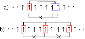
Figure 1: Configurations of spins described in the text and whose entanglement properties are presented in Fig. 2. We fix the range of spin/spin entanglement $R\leq 3$ such that spins at a distance $d\geq 4$ are not directly entangled. a) ’Clustering’ two spins increases the range of entanglement (the scheme is symmetric also for spins on the left of the marked one). b) Symmetric configuration of spins such that no two-particle entanglement is present, but still the spins share multiparticle entanglement.

An interesting case is when there is no two-particle entanglement between of any the three spins, but still they share ME. Specifically, we consider the symmetric configuration of spins drawn in Fig.1b. As shown in Fig.2 (lower panel), the Negativity between the central spin and the other two $\mathcal{N}_{Centr}$ and between an external spin and the other two $\mathcal{N}_{Ext}$ may be non-zero, despite the three spins do not share spin-spin entanglement.

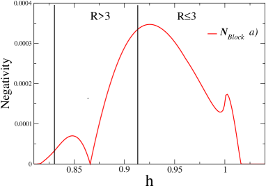
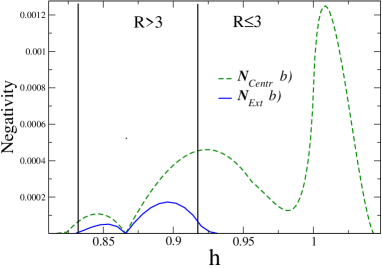
Figure 2: $T=0$ Negativities between one spin and the other two Vs magnetic field $h$ are shown for both configurations of Fig 1. We consider $\gamma=0.5$. In this case outside the interval marked by the two solid vertical lines ( $0.83\lesssim h\lesssim 0.91$) the range of spin-spin entanglement is $R\leq 3$ (for values of $h$ inside this interval $R$ grows due to the its divergence at factorizing field $h_{f}=\sqrt{1-\gamma^{2}}\simeq 0.86$ DIV ). For configuration $a)$ (upper panel), $\mathcal{N}_{Block}$ signals the spin/block entanglement for a distance $d=4$. For values of $h$ outside the vertical lines, the Negativity signals genuine spin/block entanglement. For configuration $b)$ (lower panel), both $\mathcal{N}_{Ext}$ (solid line) and $\mathcal{N}_{Centr}$ (dashed line) are plotted. For values of $h$ outside the vertical lines the three spins share no spin/spin entanglement, hence for non zero $\mathcal{N}_{Ext}$ and $\mathcal{N}_{Centr}$ free multiparticle entanglement is present. The latter turns in to bound entanglement for values of $h$ such that only $\mathcal{N}_{Centr}\neq 0$ and $\mathcal{N}_{Ext}=0$ (both on the left and on the right of the solid lines).

We shall see that spins in the configuration of Fig. 1 b) can share bound entanglement. To prove it, the idea is to resort the ”incomplete separability” condition described in the first section. In fact from Fig. 2 we see that $\mathcal{N}_{Ext}$ may be zero even if $\mathcal{N}_{Centr}$ is non-zero. Thus in such case the density matrix of the spins is PPT for the two symmetric bipartitions of one external spin vs the other two ($\uparrow|\uparrow\uparrow$ and $\uparrow\uparrow|\uparrow$) and Negative Partial Transpose (NPT) for the partition of the central spin vs the other two. We remark that PPT does not ensure the separability of the two partitions, nevertheless the state is bound entangled. In fact if we could be able to distill a maximally entangled state between two spins then one of two previous PPT partitions would be NPT and this cannot occur since PPT is invariant under LOCC HORO1 ; WERNER .

The scenario described above quantitatively varies if different values of $\gamma$ are considered. Since the range of spin-spin entanglement depends on $\gamma$ DIV the distance between the spins at which ME exists and its range are also $\gamma$-dependent. For both the configurations we studied we found that ME is short ranged. However, we notice that such range diverges at the factorizing field $h_{f}$ (analogously to what occurs for spin/spin entanglement DIV ). Remarkably, this holds also for BE. In fact we observe that the range of $\mathcal{N}_{Centr}$ is always greater than the range of $\mathcal{N}_{Ext}$. Hence approaching $h_{f}$ there are always configurations of spin far apart enough to share BE and for $h\rightarrow h_{f}$ its range diverges.

In summary if the spins are far enough to loose all spin-spin entanglement, some ME may be still present. The nature of the entanglement may change from free to bound entanglement by tuning the magnetic field $h$.

III.2 Thermal Bound Entanglement

Quantum states must be ’mixed enough’ to be bound entangled. In fact in a geometrical picture they may be located in a region separating free entangled states from the separable ones GEOMETRICAL-BOUND . In our case, a source mixing is the trace over the other spins of the chain: as pointed out in the previous section, such loss of information may be enough to induce bound entanglement between the three spins. However if the spins are near enough the reduced entanglement is free. Thus in this situation it is intriguing to investigate whether the effect of the thermal mixing can drive the $T=0$ free entanglement to BE. To answer this question we consider a block of three adjacent spins and study the entanglement between them as a function of $T$. We see (Fig. 3) that the entanglement between the two external spins is the most fragile increasing $T$, dying first at a certain $T_{C2}$; then at a higher temperature $T_{C1}$ the central spin looses its entanglement with each of the external ones. Thus for $T>T_{C1}$ there is no two-particle entanglement between the spins, but still some ME is present, as detected by the Negativity $\mathcal{N}_{Ext}$ and $\mathcal{N}_{Centr}$. Eventually the Negativity vanishes at $T_{\mathcal{N}_{Ext}}$ and $T_{\mathcal{N}_{Centr}}$. In the region $T_{\mathcal{N}_{Ext}}<T<T_{\mathcal{N}_{Centr}}$ the condition of ’incomplete separability’ occurs: the density matrix is PPT with respect to the external bipartitions and NPT with respect to the central one and thus the spins share BE.

We want to remark here that the failure of Negativity to detect some entangled states does not invalidate the scheme described above. In fact, when all the Negativities are eventually zero, the three-spin state may be still entangled, but such entanglement would be surely bound (since the state has positive partial transpose). This means that the region where bound entanglement is present might be wider than the one marked in Fig. 3, but, any case, such thermal bound entanglement will always separate the high temperature separable region from the low temperature free entangled one.

This behavior shown for the Ising model is also found for the entire class of Hamiltonians (2). In fact although the temperature at which the different types of entanglement are suppressed is $\gamma$ dependent the qualitative behavior of the phenomenon is a general feature of the model (2).

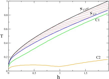
Figure 3: Entanglement shared in a block of the three adjacent spins. We consider $\gamma=1$. In this case only nearest neighbor and next nearest neighbor spins are entangled (hence $R=2$) at $T=0$ NATURE ; OSBORNE02 . The lines in the $T-h$ plane indicate the temperatures at which the corresponding type of entanglement disappears. In the marked region $T_{\mathcal{N}_{Ext}}<T<T_{\mathcal{N}_{Centr}}$ BE is present.

IV Conclusions

We studied the entanglement shared between three spins in an infinite chain described by the anisotropic XY model in a transverse field. We analyzed the Negativity between groups of spins as in Fig.1, demonstrating that the corresponding block/block entanglement extends along the chain over a longer range (Fig. 2) compared to the spin/spin case. Such type of entanglement persists at higher temperature (see Fig. 3).

In a recent paper, thermal BE was found for system made of few spins TOTH07 . Here we proved the existence of bound entanglement shared between the particles, even in a macroscopic system. It occurs naturally in certain region of the phase diagram for the ’last’ entangled states before the complete separability is reached. In this sense the BE bridges between quantum and classical correlations. Being the BE a form of demoted entanglement, we found that it appears when quantum correlations get weaker. At zero temperature bound entanglement appears (see Fig. 2) when the spins are sufficiently distant each others and as in the case of the spin/spin entanglement, it can be arbitrary long ranged near the factorizing field. At $T\neq 0$ BE is present when the system is driven toward a completely mixed state as the temperature is raised(Fig. 3). It would be an interesting to further study bound entanglement in this context (f.i. focusing on other kinds of bound entanglement UPB ).

A more refined classification of ME could be done following the scheme of Ref.ACIN , discerning different regions in the phase diagram in terms of different entanglement classes (GHZ or W). In Ref. ACIN certain witness operators able to distinguish some $W$- and $GHZ$- mixed states were discussed. We point out, however, that in our case such witness are not able to detect tripartite entanglement, not even if suitably generalized as VERTESI . Instead, the three tangleKKW , that in principle could identify the GHZ class, is difficult to handle for generic mixed state and requires a hard numerical effort (some progress is achieved for low rank density matricesJENS ).

It is plausible that increasing the size of the subsystem considered will increase the range of the ME. For instance, the range of spin/block entanglement (see configuration of Fig. 1 a) will increase if we consider a larger block. Hence, a single spin can be entangled with more distant partners, if one allow to cluster them into a large enough block. It would be intriguing to study how spin/block entanglement and, in general, block/block entanglement between subsystems, scale increasing the size of blocks. especially exploring the connection with quantum criticality. We remark that such analysis would be different with respect to the well known block entropy settingVIDAL ; BLOCK , since in that case one is interested in the block/rest-of-the-system entanglement. Along this line, some results for a chain of coupled harmonic oscillators were obtainedWERNER-CHAIN .

Finally, we speculate about the effect of temperature for the entanglement of a larger size block of spins. The behavior depicted in Fig. 3 suggests that entanglement between sub-blocks of few spins will be suppressed by increasing the temperature, before of the entanglement between larger sub-blocks. Namely, temperature will suppress first spin/spin entanglement, then spin/2-spinblock entanglement,.., n-spinblock/m-spinblock entanglement, and so on. Thus, at high enough temperature, particles of the system will eventually loose all entanglement passing through successive steps at which temperature suppresses entanglement with respect to a ’microscopic’ to ’macroscopic’ hierarchy.

Appendix

It is convenient to express $\rho_{ijk}$ in terms of three-point correlation functions that can be obtained explicitly following the method used for the two-point correlation functions in MODELLO

$$\rho_{ijk}=\sum_{pqr}\langle\sigma^{p}_{i}\sigma^{q}_{j}\sigma^{r}_{k}\rangle\sigma^{p}\otimes\sigma^{q}\otimes\sigma^{r}\;\;.$$ (3)

In the previous equation $p$,$q$,$r$$=0,x,y,z$ ($\sigma^{0}=\textbf{1}$).

Three-spin reduced density matrix is obtained from Eq.(3). Due to the parity symmetry of the Hamiltonian VIDAL2 , for the non-broken symmetry case some of the correlators are identically zero and the $8\times 8$ matrix reads:

$$\rho_{ijk}=\frac{1}{8}\left(\begin{array}[]{cc}\rho_{I}&\rho_{III}\\ \rho_{III}&\rho_{II}\end{array}\right),$$

where

$$\rho_{I} =$$

$$\hskip-35.0pt\left(\begin{array}[]{cccc}1+\mathcal{A}+\mathcal{B}^{++}&0&0&\mathcal{D}^{-}_{\beta}+\mathcal{E}^{-}_{\beta\alpha}\\ 0&1+\mathcal{C}+\mathcal{B}^{--}&\mathcal{D}^{+}_{\beta}+\mathcal{E}^{+}_{\beta\alpha}&0\\ 0&\mathcal{D}^{+}_{\beta}+\mathcal{E}^{+}_{\beta\alpha}&1+\mathcal{C}-\mathcal{B}^{+-}&0\\ \mathcal{D}^{-}_{\beta}+\mathcal{E}^{-}_{\beta\alpha}&0&0&1-\mathcal{C}-\mathcal{B}^{-+}\\ \end{array}\right)$$

$$\rho_{II} =$$

$$\hskip-35.0pt\left(\begin{array}[]{cccc}1+\mathcal{C}-\mathcal{B}^{-+}&0&0&\mathcal{D}^{-}_{\beta}-\mathcal{E}^{-}_{\beta\alpha}\\ 0&1-\mathcal{C}-\mathcal{B}^{+-}&\mathcal{D}^{-}_{\beta}-\mathcal{E}^{+}_{\beta\alpha}&0\\ 0&\mathcal{D}^{-}_{\beta}-\mathcal{E}^{+}_{\beta\alpha}&1-\mathcal{C}+\mathcal{B}^{--}&0\\ \mathcal{D}^{-}_{\beta}-\mathcal{E}^{-}_{\beta\alpha}&0&0&1-\mathcal{A}+\mathcal{B}^{++}\\ \end{array}\right)$$

$$\rho_{III} =$$

$$\hskip-20.0pt\left(\begin{array}[]{cccc}0&\mathcal{D}^{+}_{\gamma}+\mathcal{F}^{+}_{\alpha\beta}&\mathcal{D}^{+}_{\alpha}+\mathcal{F}^{+}_{\alpha\beta}&0\\ \mathcal{D}^{-}_{\gamma}+\mathcal{F}^{-}_{\alpha\beta}&0&0&\mathcal{D}^{+}_{\alpha}-\mathcal{F}^{+}_{\alpha\beta}\\ \mathcal{D}^{-}_{\alpha}+\mathcal{F}^{-}_{\alpha\beta}&0&0&\mathcal{D}^{+}_{\gamma}+\mathcal{F}^{+}_{\alpha\beta}\\ 0&\mathcal{D}^{-}_{\alpha}-\mathcal{F}^{-}_{\alpha\beta}&\mathcal{D}^{-}_{\gamma}-\mathcal{F}^{-}_{\alpha\beta}&0\\ \end{array}\right).$$

The entries of the matrices above are linear combination of the correlation functions:

$$\mathcal{A} = 3Z+ZZZ$$

$$\mathcal{B}^{\pm\pm} = ZZ_{\alpha}\pm ZZ_{\beta}\pm ZZ_{\gamma}$$

$$\mathcal{C} = Z-ZZZ$$

$$\mathcal{D}^{\pm}_{\alpha} = XX_{\alpha}\pm YY_{\alpha}$$

$$\mathcal{E}^{\pm}_{\alpha\beta} = XXZ_{\alpha\beta}\pm YYZ_{\alpha\beta}$$

$$\mathcal{F}^{\pm}_{\alpha\beta} = XZX_{\alpha\beta}\pm YZY_{\alpha\beta}$$

where f.i. $YYZ_{\alpha\beta}=\langle\sigma^{y}_{i}\sigma^{y}_{j}\sigma^{z}_{k}\rangle$ with $\alpha=j-i$ and $\beta=k-j$ (the correlators depend only on the relative distance between the spins because of the translational symmetry of the system).

Such three-point correlation functions can be calculated following the method used in MODELLO for the two-point ones. In short, after the Jordan-Wigner transformation which maps spin into spinless fermions

$$\sigma_{l}^{x} = A_{l}\prod_{s=1}^{l-1}A_{s}B_{s}$$

$$\sigma^{y} = -B_{l}\prod_{s=1}^{l-1}A_{s}B_{s}$$

$$\sigma^{z} = -A_{l}B_{l}\;.$$

where $A=c+c^{\dagger}$ and $B=c-c^{\dagger}$, the three-point correlation functions $\langle\sigma^{p}_{i}\sigma^{q}_{j}\sigma^{r}_{k}\rangle$ can be written as a Pfaffian whose elements are the two-point correlators $\langle A_{l}B_{m}\rangle$. The structure of the Pfaffians further simplifies in to a determinant because only terms $\langle A_{l}B_{m}\rangle=G_{m-l}=\int^{\pi}_{0}\ \frac{1}{\pi}\{\cos(\phi|m-l|)(\cos(\phi)-a)-\gamma\sin(\phi|m-l|)\sin(\phi)\}\frac{\tanh(\frac{1}{2T}\sqrt{\gamma^{2}\sin\phi^{2}+(h-\cos\phi^{2})})}{\sqrt{\gamma^{2}\sin\phi^{2}+(h-\cos\phi^{2})}}d\phi$ are non vanishing.

$$ZZZ_{\alpha\beta} = -\left|\begin{array}[]{ccc}G_{0}&G_{\alpha}&G_{\alpha+\beta}\\ G_{-\alpha}&G_{0}&G_{\beta}\\ G_{-\alpha-\beta}&G_{-\beta}&G_{0}\\ \end{array}\right|,$$

$$XXZ_{\alpha\beta} = (-)^{\alpha+1}\times$$

$$\hskip-20.0pt\left|\begin{array}[]{ccccc}G_{-1}&G_{0}&\ldots&G_{\alpha-2}&G_{\alpha+\beta-1}\\ G_{-2}&G_{-1}&\ldots&G_{\alpha-3}&G_{\alpha+\beta-2}\\ \vdots&&\ddots&\vdots&\vdots\\ G_{-\alpha}&G_{-\alpha-1}&\ldots&G_{-1}&G_{\beta}\\ G_{-\alpha-\beta}&G_{-\alpha-\beta-1}&\ldots&G_{-\beta-1}&G_{0}\\ \end{array}\right|,$$

$$XZX_{\alpha\beta} = (-)^{\alpha+\beta}\times$$

$$\hskip-20.0pt\left|\begin{array}[]{ccccccc}G_{-1}&\ldots&G_{\alpha-2}&G_{\alpha}&\ldots&G_{\alpha+\beta-2}\\ \vdots&&\vdots&\vdots&&\vdots\\ G_{-\alpha+1}&\ldots&G_{0}&G_{2}&\ldots&G_{\beta}\\ G_{-\alpha-1}&\ldots&G_{-2}&G_{0}&\ldots&G_{\beta-2}\\ \vdots&&\vdots&\vdots&&\vdots\\ G_{-\alpha-\beta}&\ldots&G_{-\beta-1}&G_{-\beta+1}&\ldots&G_{-1}\\ \end{array}\right|,$$

$$YYZ_{\alpha\beta} = (-)^{\alpha+1}\times$$

$$\hskip-20.0pt\left|\begin{array}[]{ccccc}G_{1}&G_{2}&\ldots&G_{\alpha}&G_{\alpha+\beta}\\ G_{0}&G_{1}&\ldots&G_{\alpha-1}&G_{\alpha+\beta-1}\\ \vdots&&\ddots&\vdots&\vdots\\ G_{-\alpha+2}&G_{-\alpha+3}&\ldots&G_{1}&G_{\beta+1}\\ G_{-\alpha-\beta+1}&G_{-\alpha-\beta+2}&\ldots&G_{-\beta}&G_{0}\\ \end{array}\right|,$$

$$YZY_{\alpha\beta} = (-)^{\alpha+\beta}\times$$

$$\hskip-20.0pt\left|\begin{array}[]{ccccccc}G_{1}&\ldots&G_{\alpha-1}&G_{\alpha+1}&\ldots&G_{\alpha+\beta}\\ \vdots&&\vdots&\vdots&&\vdots\\ G_{-\alpha+2}&\ldots&G_{0}&G_{2}&\ldots&G_{\beta+1}\\ G_{-\alpha}&\ldots&G_{-2}&G_{0}&\ldots&G_{\beta-1}\\ \vdots&&\vdots&\vdots&&\vdots\\ G_{-\alpha-\beta+2}&\ldots&G_{-\beta}&G_{-\beta+2}&\ldots&G_{1}\\ \end{array}\right|.$$

The main difference with respect the two-point correlators calculated in MODELLO is that in this case the Toeplitz structure of the matrix is no longer valid.

References

- (1) M. A. Nielsen and I. Chuang, Quantum Computation and Quantum Communication, Cambridge University Press, Cambridge, (2000).
- (2) L. Amico, R. Fazio, A. Osterloh, and V. Vedral, Entanglement in many-body systems, arXiv:quant-ph/0703044.
- (3) A. Osterloh, L. Amico, G. Falci, and R. Fazio, Nature (London) 416, 608 (2002).
- (4) T.J. Osborne and M.A. Nielsen, Phys. Rev. A 66,032110 (2002).
- (5) G. Vidal, J.I. Latorre, E. Rico, and A. Kitaev, Phys.Rev.Lett. 90, 227902 (2003).
- (6) T. J. Osborne and F. Verstraete, Phys. Rev. Lett.96, 220503 (2006).
- (7) V. Coffmann, J. Kundu and W.K. Wootters, Phys. Rev. A 61, 052306 (2000).
- (8) T. Roscilde, P. Verrucchi, A. Fubini, S. Haas, and V. Tognetti, Phys. Rev. Lett.93, 167203 (2004).
- (9) A. Anfossi et al., Phys. Rev. Lett. 95, 056402 (2005).
- (10) T. R. de Oliveira, G. Rigolin, M. C. de Oliveira, and E. Miranda Phys. Rev. Lett. 97, 170401 (2006).
- (11) T. C. Wei, D. Das, S. Mukhopadyay, S. Vishveshwara, and P. M. Goldbart, Phys. Rev. B 71, 060305(R) (2005).
- (12) H. Barnum and E. Knill and G. Ortiz and R. Somma and L. Viola, Phys. Rev. Lett. 92, 107902 (2004).
- (13) R. Somma and G. Ortiz and H. Barnum and E. Knill and L. Viola, Phys. Rev. A 70, 042311 (2004).
- (14) S. Montangero and L. Viola Phys. Rev. A 73, 040302(R) (2006).
- (15) O. Guehne, G. Tóth and H.J. Briegel, New. J. Phys. 7, 229 (2005).
- (16) O. Guehne and G. Tóth, Phys. Rev. A 73, 052319 (2006).
- (17) P. Facchi, G. Florio and S. Pascazio, Phys. Rev. A 74, 042331 (2006); G. Costantini and P. Facchi and G. Florio and S. Pascazio, quant-ph/0612098.
- (18) C. Lunkes, C. Brukner and V. Vedral, Phys. Rev. Lett.95, 030503 (2005).
- (19) V. Vértesi, quant-ph/0701246
- (20) M. Horodecki et al., Phys. Rev. Lett. 80, (24) 5239-5242 (1998).
- (21) W. Dür and J.I. Cirac, Phys. Rev. A 61, 042314 (2000).
- (22) R. Horodecki, P. Horodecki, M. Horodecki and K. Horodecki, quant-ph/0702225v2
- (23) M. Horodecki, P. Horodecki, and R. Horodecki, Phys. Rev. Lett. 82, 1056 (1999).
- (24) K. Horodecki, M. Horodecki, and P. Horodecki, and J. Oppenheim, Phys. Rev. Lett. 94, 160502 (2005).
- (25) L. Masanes, Phys. Rev. Lett.96, 150501 (2006).
- (26) P. Hyllus, C. Moura Alves, D. Bruss and C. Macchiavello, Phys. Rev. A 70, 032316 (2004).
- (27) W.K. Wootters, Phys. Rev. Lett. 80, 2245 (1998).
- (28) C. H. Bennett et al., Phys. Rev. A 53, 2046 (1996).
- (29) W. Dür, J.I. Cirac, M. Lewenstein, and D. Bruss, Phys Rev. A 61, 062313 (2000).
- (30) W. Dür, Phys. Rev. Lett.87, 230402 (2001).
- (31) L. Masanes, Phys. Rev. Lett.97, 050503 (2006).
- (32) G. Vidal and R.F. Werner, Phys. Rev. A 65, 032314 (2002).
- (33) J. Eisert, quant-ph/0610253.
- (34) For a more refined analysis see Ref.ACIN .
- (35) Y. Ou and H. Fan, quant-ph/0702127v4.
- (36) E. Lieb, T. Schulz, and D. Mathis, Ann. Phys. 60, 407 (1961); P. Pfeuty, Ann. Phys. 57, 79 (1970); E. Barouch and B.M. McCoy, Phys. Rev. A 3, 786 (1971).
- (37) L. Amico et al., Phys. Rev. A 74, 022322 (2006).
- (38) J. Kurmann, H. Thomas and G. Müller, Physica A, 112, 235 (1982).
- (39) A. R. Its, B.-Q. Jin and V. E. Korepin, Journal Phys. A: Math. Gen. vol 38, pages 2975-2990, (2005).
- (40) J.M. Leinaas et al., quant-ph/0605079.
- (41) G. Tóth et al., arXiv:quant-ph/0702219.
- (42) C.H. Bennett et al., Phys. Rev. Lett.82, 5385 (1999); S. Bravyi, Quant. Inf. Processing 3 309 (2004).
- (43) A. Acín, D. Bruss, M. Lewenstein, and A. Sanpera, Phys. Rev. Lett. 87, 040401 (2001).
- (44) R. Lohmayer, A. Osterloh, J. Siewert, A. Uhlmann, Phys. Rev. Lett. 97, 260502, (2006).
- (45) V. Korepin, Phys. Rev. Lett. 97, 096402, (2004); B.-Q.Jin and V.E.Korepin, J. Stat. Phys. 116, 79 (2004); M. B. Plenio et al., Phys. Rev. Lett. 94, 060503 (2005); M.M. Wolf, Phys. Rev. Lett. 96, 010404 (2006).
- (46) K. Audenaert et al., Phys Rev. A 66, 042327 (2002).
- (47) J. I. Latorre, E. Rico and G. Vidal, Quant. Inf. and Comp. 4 048 (2004).