Constraining dark energy via baryon acoustic oscillations in the (an)isotropic light-cone power spectrum

Abstract

Context. The measurement of the scale of the baryon acoustic oscillations (BAO) in the galaxy power spectrum as a function of redshift is a promising method to constrain the equation-of-state parameter of the dark energy $w$.

Aims. To measure the scale of the BAO precisely, a substantial volume of space must be surveyed. We test whether light-cone effects are important and whether the scaling relations used to compensate for an incorrect reference cosmology are in this case sufficiently accurate. We investigate the degeneracies in the cosmological parameters and the benefits of using the two-dimensional anisotropic power spectrum. Finally, we estimate the uncertainty with which $w$ can be measured by proposed surveys at redshifts of about $z=3$ and $z=1$, respectively.

Methods. Our data is generated by cosmological N-body simulations of the standard $\Lambda$CDM scenario. We construct galaxy catalogs by “observing” the redshifts of different numbers of mock galaxies on a light cone at redshifts of about $z=3$ and $z=1$. From the “observed” redshifts, we calculate the distances, assuming a reference cosmology that depends on $w_{\rm ref}$. We do this for $w_{\rm ref}=-0.8,-1.0$, and $-1.2$ holding the other cosmological parameters fixed. By fitting the corresponding (an)isotropic power spectra, we determine the apparent scale of the BAO and the corresponding $w$.

Results. In the simulated survey we find that light-cone effects are small and that the simple scaling relations used to correct for the cosmological distortion work fairly well even for large survey volumes. The analysis of the two-dimensional anisotropic power spectra enables an independent determination to be made of the apparent scale of the BAO, perpendicular and parallel to the line of sight. This is essential for two-parameter $w$-models, such as the redshift-dependent dark energy model $w=w_{0}+(1-a)w_{a}$. Using Planck priors for the matter and baryon density and $\Delta H_{0}=5\%$ for the Hubble constant, we estimate that the BAO measurements of future surveys around $z=3$ and $z=1$ will be able to constrain, independently of other cosmological probes, a constant $w$ to $\sim 12\%$ and $\sim 11\%$ (68% c.l.), respectively.

1 Introduction

There are two main observational indications of the existence of an unknown energy component in the Universe, which is usually referred to as dark energy (DE). First, observations of distant supernovae Ia (Riess et al. 1998; Perlmutter et al. 1999) favor an accelerating expansion of the Universe and therefore imply an energy component of negative pressure $P$. In particular, the parameter $w$ of the equation of state (EOS) $P=w\rho$ must obey $w<-1/3$. Second, measurements of the anisotropies in the cosmic microwave background (CMB) (Spergel et al. 2003, 2007) in combination with observations of the large-scale structure of the Universe argue for a spatially flat Universe. Matter (baryonic and dark) contributes however less than 30% to the critical density. Hence, about 70% of the present-day energy density of the Universe appears to be in an unknown form of energy. The simplest way to account for this missing energy and the accelerating expansion is to introduce a cosmological constant $\Lambda$ in Einstein’s equations, which has a redshift-independent EOS parameter $w=-1$. So far all observations appear to agree with the model of a cosmological constant. There is however at least one theoretical drawback. The observed value of $\Lambda$, which is interpreted as vacuum energy, is highly inconsistent with current predictions by particle physics, a discrepancy commonly referred to as the cosmological constant problem (for a review, see Carroll (2001)). This has motivated consideration of more general dark energy models that have a redshift-dependent EOS parameter $w(z)$. The measurement of the parameter $w$ can therefore help to distinguish between not only a simple cosmological constant and other dark energy models, but potentially also between these different models.

Several possible methods to constrain the EOS parameter $w$ are summarized by the Dark Energy Task Force Report (Albrecht et al. 2006). The method that we consider here uses the expansion history of the Universe. To measure this precisely, we require a standard candle or a standard ruler. For redshifts up to $z\sim 1.8$, supernovae Ia can be observed and calibrated to be standard candles, with which one can measure the luminous distance $D_{L}(z)$. Eisenstein et al. (1998, 1999) proposed that the baryon acoustic oscillations (BAO) imprinted in the galaxy power spectrum could be utilized as a standard ruler. The BAO have the same origin as the acoustic peaks in the anisotropies of the CMB. Before recombination, baryons and photons were tightly coupled. Gravitation and radiation pressure produced acoustic oscillations in this hot plasma; during the expansion of the Universe, the plasma then cooled and finally nuclei and electrons recombined. The released photons propagated through the expanding Universe and are observed by ourselves as the highly redshifted radiation of the CMB; in contrast, the baryons followed the clustering of the dark matter and eventually collapsed to form galaxies. Since the dark matter did not participate in the acoustic oscillations, the oscillatory feature in the galaxy power spectrum is far less pronounced than for the CMB photons (Peebles & Yu 1970; Sunyaev & Zeldovich 1970; Bond & Efstathiou 1984; Holtzman 1989; Hu & Sugiyama 1996; Eisenstein & Hu 1998).

When the physical scale of the BAO has been calibrated using precise CMB measurements, it can be applied as a standard ruler for measuring the angular diameter distance $D_{A}(z)$ and Hubble parameter $H(z)$. In contrast to supernovae Ia, the scale of the BAO is a more reliable standard ruler at high redshifts. As the number of unperturbed peaks and troughs corresponding to the BAO in the power spectra increases, the wavelength of the BAO can be determined more accurately. On scales where structure growth is already nonlinear, the oscillations cannot be easily discerned (Springel et al. 2005; Gottlöber et al. 2006; Eisenstein et al. 2007b). Hence, with decreasing redshift the uncertainty in the observed scale of the BAO increases. To have good statistics for the first peaks a large volume has to be surveyed. The BAO have been detected in the present-day largest galaxy redshift surveys (Eisenstein et al. 2005; Cole et al. 2005). Data sets studying larger volumes and higher redshifts are however required to achieve tight constraints on dynamical DE models. Galaxy redshift surveys at about $z=3$, $1$, or $0.5$, like HETDEX (Hill et al. 2004), the WFMOS BAO survey (Glazebrook et al. 2005; Bassett et al. 2005), and BOSS (SDSS-III Collaboration 2008), are designed for measuring the scale of the BAO and the EOS parameter $w$ with a precision to a few percent and thereby constrain a variety of DE models.

Many studies presented methods for extracting the scale of the BAO and estimated the accuracy of its measurement achievable by future surveys. In these analyses, Monte Carlo simulations (Blake & Glazebrook 2003; Glazebrook & Blake 2005; Blake et al. 2006), Fisher matrix techniques (Linder 2003; Hu & Haiman 2003; Seo & Eisenstein 2003; Matsubara 2004; Hütsi 2006b; Seo & Eisenstein 2007), N-body simulations (Angulo et al. 2005; White 2005; Seo & Eisenstein 2005; Huff et al. 2007; Koehler et al. 2007; Angulo et al. 2008), and observational data (Eisenstein et al. 2005; Hütsi 2005, 2006a, 2006c) were used.

In this article, we attempt to include all important (physical and observational) effects for measuring the BAO and deriving constraints on the EOS parameter $w$. Our perspective is that of an observer, i.e. the starting point for the BAO measurement should be a galaxy catalog that provides celestial coordinates and redshifts of the galaxies. Since we do not have in hand the type of real observations that we require, we have first to generate mock catalogs; we achieve this by completing “observations” on the data products of N-body simulations. Using these “observations”, we are able to study for the first time in detail the light-cone effect and the accuracy of the scaling relations used to compensate the cosmological distortion that arises by assuming an incorrect reference cosmology. A crucial point for all BAO measurements is the fitting method. We develop a method which uses only the oscillatory part of the power spectrum in a way that produces unbiased and robust results. Further, we compare the results of fitting the angle-averaged one-dimensional power spectrum and anisotropic two-dimensional power spectrum. Finally, we predict the uncertainty with which proposed surveys will be able to measure the EOS parameter $w$ by assuming two different $w$-models.

The paper is structured as follows. In Sect. 2, we review how the EOS parameter $w$ is measured using BAO. In Sect. 3, we explain how we generate the “observed” data from N-body simulations, and in Sect. 4, we describe the power spectrum calculation and our fitting method. In Sect. 5, we present our results, and finally we provide our conclusions in Sect. 6.

2 Cosmology with baryon acoustic oscillations

Knowledge of the true comoving scales, both parallel ($r_{\parallel}$) and transverse ($r_{\bot}$) to the line of sight, of an observed physical property at a given redshift $z$, in the case of BAO statistical properties of large-scale structure, enables us to derive the Hubble parameter $H(z)$ and angular diameter distance $D_{A}(z)$ from the measured quantities (redshift $\Delta z$ and angle $\Delta\theta$) :

$$\begin{aligned} r_{\parallel}&=\frac{c\Delta z}{H(z)}\,,\\ r_{\bot}&=(1+z)D_{A}(z)\Delta\theta\,.\end{aligned}$$ (1)

In a flat Universe and for moderate redshifts at which the contribution of radiation can be neglected, the Hubble parameter depends on three cosmological parameters, the present-day Hubble parameter $H_{0}$, fraction of matter $\Omega_{\rm m}$, and the dark energy EOS parameter $w$(z), in the following manner

$$H(z)=H_{0}\sqrt{\Omega_{\rm m}(1+z)^{3}+(1-\Omega_{\rm m})\exp\left(3\int_{0}^{z}{\frac{1+w(\tilde{z})}{1+\tilde{z}}\,{\rm d}\tilde{z}}\right)}\,.$$ (2)

The angular diameter distance $D_{A}(z)$ is a functional of the Hubble parameter and is given by

$$D_{A}(z)=\frac{c}{1+z}\int_{0}^{z}{\frac{{\rm d}\tilde{z}}{H(\tilde{z})}}\,.$$ (3)

Assuming that we know apart from $w$ all important cosmological parameters to significant precision from other observations, especially from CMB precision measurements such as WMAP (Spergel et al. 2007) and direct measurements of the Hubble constant $H_{0}$ by the HST Key project (Freedman et al. 2001), one can constrain the EOS parameter $w$ using this chain of equations. Since $w$ appears in an integral over $z$ in Eq. (2), observations at a single redshift cannot be used to measure the value of $w$ at this redshift. A certain model for $w$ has to be assumed before its value can be measured. In this paper, we assume a constant $w$ and a simple redshift-dependent parameterization $w=w_{0}+(1-a)w_{a}$; this parameterization is used frequently in the literature (compare Dark Energy Task Force Report (Albrecht et al. 2006)) and advocated by Linder (2007) to be robust and applicable to a wide range of dark energy models.

One problem of using the scale of the BAO as a standard ruler is that the BAO appear in a statistical quantity. We cannot measure $\Delta z$ of the BAO, but we can measure the redshifts of the galaxies and then, assuming a reference cosmology, reconstruct their positions and derive their power spectrum. From this power spectrum, we can determine the apparent scale of the BAO and compare this with its true value. If they agree, we have used the correct cosmology. In principle, for every trial cosmology we have to recalculate the distances and recompute the power spectrum. A more efficient method is to scale appropriately the power spectrum derived for the reference cosmology using the following approximations (Seo & Eisenstein 2003; Glazebrook & Blake 2005)

$$\begin{aligned} k_{\parallel}=\frac{H(z)}{H^{\rm ref}(z)}k_{\parallel}^{\rm ref}\,,\quad k_{\bot}=\frac{D_{A}^{\rm ref}(z)}{D_{A}(z)}k_{\bot}^{\rm ref}\,.\end{aligned}$$ (4)

In this paper, we test if these approximations are still sufficiently accurate for very large surveys where $z$ varies substantially within the survey. We achieve this by using three reference cosmologies, which differ only in the EOS parameter $w_{\rm ref}=-0.8,\,-1.0,\,-1.2$. We use the relation (4) to scale the derived power spectra and compare the results. For convenience, we define the following scaling factors parallel and transverse to the line of sight and an isotropic one for the one-dimensional angle-averaged power spectrum

$$\begin{aligned} \lambda_{\parallel}&=\frac{H(z)}{H^{\rm ref}(z)}\,,\quad\lambda_{\bot}=\frac{D_{A}^{\rm ref}(z)}{D_{A}(z)}\,,\\ \lambda_{\rm iso}&=(\lambda_{\bot}^{2}\lambda_{\parallel})^{1/3}\,.\end{aligned}$$ (5)

In Fig. 1, we show the dependence of the scaling factors on a constant $w$ for redshift $z=3$ (solid line) and $z=1$ (dotted line). As a reference value, we chose $w_{\rm ref}=-1.0$. We also show the derivatives of the scaling factors with respect to $w$. The higher the value of the derivative, the more accurately we can constrain the constant $w$ for a given uncertainty in the scaling factor. Since the derivatives decrease with decreasing $w$, the uncertainty in $w$ will be, in general, higher towards lower $w$ values. The derivative of $\lambda_{\rm iso}$ around $w=-1$ at redshift $z=1$ is $\sim 1.5$ times higher than at $z=3$, that is although we can probably measure the scale of the BAO less accurately at redshift $z=1$ than at $z=3$ (due to nonlinear evolution), this does not need to be the case for the EOS parameter $w$.

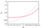
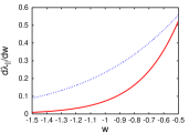
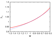
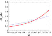
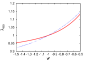
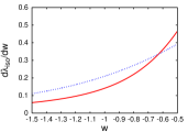
Figure 1: The scaling factors $\lambda_{\parallel,\bot}$ and $\lambda_{\rm iso}$ and their derivatives are shown as a function of $w$ for the redshifts $z=3$ (solid line) and $z=1$ (dotted line).

3 Simulation data

To derive realistic samples of large galaxy surveys, we first completed an N-body simulation in a large box ($1.5\,\mathrm{Gpc}/h$) and constructed the corresponding dark matter distribution on a light cone by interpolating between about $20$ snapshots. We calculated the redshifts, which would be observed including the effect of peculiar velocities. Assuming a certain cosmology, we converted these redshifts into distances. Finally, we selected a certain number of particles by applying a simple bias scheme and defining them as galaxies. In the following subsections, we describe each step of this procedure.

3.1 N-body simulation

Our principal N-body simulation consists of $512^{3}$ dark matter particles of a mass of $2\times 10^{12}M_{\sun}/h$ in a $(1.5\,\mathrm{Gpc}/h)^{3}$ box. The initial power spectrum was produced by CMBfast (Seljak & Zaldarriaga 1996). Starting from a glass distribution, the particles were displaced according to second order Lagrangian perturbation theory by using the code of Sirko (2005). As cosmological parameters, we chose $\Omega_{\rm m}=0.27$, $\Omega_{\Lambda}=0.73$, $h=0.7$, $\Omega_{\rm b}h^{2}=0.023$, $n_{s}=0.95$, $\sigma_{8}=0.8$ and $w=-1.0$. The simulation was performed with GADGET-2 (Springel 2005) using a softening length of comoving $100\,\mathrm{kpc}/h$. The starting redshift was $z=20$.

We also completed twelve $256^{3}$ dark matter particles simulations with the same cosmological parameters but different realizations of the initial conditions. We used these simulations to investigate systematic effects. Especially, we tested if our fitting procedure provides unbiased results.

3.2 Light-cone survey

An observer at the present epoch $t_{0}$ ($z(t_{0})=0$) identifies the galaxy distribution on his past light cone. He receives photons emitted at $t<t_{0}$ that have traversed the comoving distance $\chi(t)=c\int_{t}^{t_{0}}{a^{-1}(\tilde{t})}\mathrm{d}\tilde{t}$. To construct a light-cone survey, we follow an approach used by Evrard et al. (2002). We identify for each particle two consecutive snapshots between which it crosses the light cone and interpolate between them to find the position and velocity of that particle on the light cone. Expressed in formulas, the interpolated position is given by $\@vec{x}=\@vec{x_{i}}+\alpha\Delta\@vec{x}$ where $\@vec{x_{i}}$ is the position of the particle in snapshot $i$ and $\Delta\@vec{x}=\@vec{x_{i+1}}-\@vec{x_{i}}$, and $\alpha$ is determined by requiring that $|\@vec{x}|=\chi(t_{i}+\alpha\Delta t)$ with $\Delta t$ being the time step between the two snapshots. After a Taylor expansion for the last term, we can solve for $\alpha$

$$\alpha=\frac{\chi^{2}(t_{i})-x_{i}^{2}}{2(\@vec{x_{i}}\cdot\Delta\@vec{x}+\chi(t_{i})\Delta\chi)}\,,$$ (6)

with $\Delta\chi=\chi(t_{i})-\chi(t_{i+1})>0$. The interpolated velocity is then given by $\@vec{v}=(1-\alpha)\@vec{v_{i}}+\alpha\@vec{v_{i+1}}$.

For the galaxy sample at redshift $z=3$, we place the center of the simulation box at redshift $z=3$, i.e. $6.4\,\mathrm{Gpc}$ comoving distance away from the virtual observer. The orientation of the box is such that the line connecting the center of the box with the observer is parallel to the $z$-axis. The $(1.5{\rm Gpc}/h)^{3}$ box then extends from redshift 2.1 to 4.7, i.e. from 5.3 Gpc to 7.6 Gpc in comoving distances. For this redshift range, we have 17 snapshots at different times, i.e. of different expansion factors: $a=0.17,0.18,\ldots 0.33$. The box centered at redshift $z=1$ ranges from redshift 0.6 to 1.7. For this interval, we use 27 snapshots with $a=0.37,0.38,\ldots 0.63$ for the light cone construction.

3.3 “Observation”

Our virtual observer is at redshift $z=0$ and the simulation box is centered on redshift $z=3$ and $z=1$, respectively. To derive a redshift for each particle, we compute the comoving distance $\chi$ to the observer and solve the following equation numerically for the expansion factor $a$,

$$\chi=c\int_{a}^{1}\frac{\mathrm{d}\tilde{a}}{\tilde{a}^{2}H(\tilde{a})}\,,$$ (7)

where $H$ is the “true” Hubble parameter of the simulation $H=H_{0}\sqrt{\Omega_{\rm m}/a^{3}+(1-\Omega_{\rm m})}$. The corresponding redshift is then $z_{H}=1/a-1$. In addition to this redshift caused by the Hubble expansion of the Universe, there is also a Doppler redshift caused by the peculiar velocity of the particle. Hence, the total observed redshift is $z=(1+z_{H})(1+{v_{\mathrm{rad}}}/{c})-1$, where $v_{\mathrm{rad}}$ is the radial velocity of the particle. The accuracy of the simulation and the numerical algorithm of the integral equation above, implies an uncertainty of $\Delta z\sim 0.001$.

We next convert the observed redshifts to distances by assuming different reference cosmologies, where the dark energy EOS parameter $w$ has the values $w_{\rm{ref}}=-0.8$, $-1.0$, and $-1.2$. In this case, the Hubble parameter becomes $H^{\rm ref}(a)=H_{0}\sqrt{\Omega_{\rm m}/a^{3}+(1-\Omega_{\rm m})/a^{3(1+w_{\mathrm{ref}})}}$.

3.4 Galaxy Bias

Since the mass resolution of our simulation is too low for identifying galaxy-sized friends-of-friends halos, we use a simple bias scheme to compile mock galaxy samples from the dark matter distribution (Cole et al. 1998; Yoshida et al. 2001). Using the initial density field, we define a probability function by $P(\nu)\propto(\nu-\nu_{\rm th})^{\alpha}$ if $\nu$ is above the threshold $\nu_{\rm th}$ and zero otherwise. The dimensionless variable $\nu$ is given by the density contrast normalized by its root-mean-square on the grid $\sigma$, i.e $\nu(\@vec{x})=\delta(\@vec{x})/\sigma$. The density contrast $\delta(\@vec{x})$ of each particle is computed in the following way. First, we assign the particles with the cloud in cell (CIC) scheme to a $512^{3}$ grid (Hockney & Eastwood 1988) to obtain the density $\rho$ on the grid points. Then, we calculate the density contrast $\delta(\@vec{x})=(\rho(\@vec{x})-\bar{\rho})/\bar{\rho}$ on the grid points and interpolate it to the positions of the particles.

In the next step, we Poisson sample the dark matter particles according to the probability function and track these “galaxies” throughout the snapshots and the constructed light cones.

As parameters, we use ($\alpha=0.3$, $\nu_{\rm th}=0.4$) for a strongly biased sample and ($\alpha=0.2$, $\nu_{\rm th}=-0.6$) for a more weakly biased sample. We calculate the corresponding galaxy bias to be the square root of the ratio of the galaxy power spectrum to the dark matter power spectrum in real space: $b^{2}=P_{\rm gal}(k)/P_{\rm dm}(k)$. The bias of the mock galaxies decreases with decreasing redshift (Fig.2) as expected in the model. We select primarily particles in high-density regions of the initial density field, which occupy less prominent structures at later times due to the further development of gravitational clustering. The bias has a mild scale dependence due to the schematic procedure of grid-based density estimation and the specific probability selection function.

The parameters $\alpha$ and $\nu_{\rm th}$ were chosen such that the strong bias sample at redshift $z=3$ is consistent with the expected bias of the target galaxies of HETDEX (Hill et al. 2004). The bias of this sample is very similar to the friends-of-friends halo sample with a halo mass higher than $\sim 4\times 10^{11}M_{\sun}/h$ obtained from the Mare Nostrum simulation (Gottlöber et al. 2006). As observations of the target galaxies of HETDEX, namely Lyman-$\alpha$ emitting galaxies (LAE), suggest (Gronwall et al. 2007; Gawiser et al. 2007), this expected value for the bias might be too optimistic. Therefore, we also use the weaker bias sample at $z=3$, which matches the measured bias of LAE observed by the MUSYC collaboration (Gronwall et al. 2007; Gawiser et al. 2007).

For $z=1$, we use the “weaker” bias sample, which is fairly consistent with the expected bias of the target galaxies of WFMOS (Bassett et al. 2005; The KAOS Purple Book 2003). The bias of the strongly biased sample at $z=1$ is too high for these galaxies and we do not use this sample in the rest of the paper.

3.5 Mock Catalogs

For the survey centered on $z=3$, we generate several mock catalogs of one million galaxies from the strongly and weakly biased light cones in redshift space using the entire $1.5\,\rm Gpc/h$ box, which has a volume of $10\,{\rm Gpc}^{3}$. These numbers are at the upper limit of the current baseline of the HETDEX project.

For the mock catalogs at $z=1$, we use only the galaxies on the light cone around $z=1$ in redshift space with a bias of $b\approx 1.5$. As a number of tracers, we choose one and two million galaxies in the entire box.

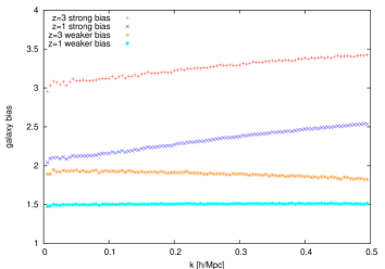
Figure 2: Galaxy bias for the two different parameter sets at redshift $z=3$ and $z=1$. To construct this plot, we used 15 million galaxies to reduce the shot noise.

4 Analyzing the data

We analyze the mock catalogs first by calculating the power spectrum and then by fitting the extracted BAO. In the following two subsections, we describe how we calculate the power spectrum and provide details about the fitting procedure.

4.1 Power spectrum

Since we use an FFT to complete the Fourier transformation, we first have to assign the particles to a regular grid. We consider a $1024^{3}$ regular grid and select the CIC scheme to complete the mass assignment. After converting the density field $\rho(\@vec{x})$ to the density contrast $\delta(\@vec{x})=(\rho(\@vec{x})-\bar{\rho})/\bar{\rho}$ and performing the FFT to evaluate the Fourier transform (FT) $\delta(\@vec{k})$, we compute the raw isotropic (one-dimensional) and anisotropic (two-dimensional) power spectrum by averaging $|\delta(\@vec{k})|^{2}$ over spherical shells $P^{\textrm{iso.}}_{\rm{raw}}(k)=\left\langle|\delta(\@vec{k})|^{2}\right\rangle_{\textrm{shell}}$ and rings $P^{\textrm{aniso.}}_{\rm{raw}}(k_{\parallel},k_{\bot})=\left\langle|\delta(\@vec{k})|^{2}\right\rangle_{\textrm{ring}}$, respectively. These raw power spectra are related to the true power spectrum in the following way (Jing 2005):

$$P^{\textrm{iso./aniso.}}_{\rm{raw}} =\left\langle\sum_{\@vec{m}\in\mathbf{Z}^{3}}|W(\@vec{k}+2k_{\rm Ny}\@vec{m})|^{2}P(\@vec{k}+2k_{\rm Ny}\@vec{m})\right.$$

$$\left.+\frac{1}{n}\sum_{\@vec{m}\in\mathbf{Z}^{3}}|W(\@vec{k}+2k_{\rm Ny}\@vec{m})|^{2}\right\rangle_{\textrm{shell/ring}}\ ,$$ (8)

where $W(\@vec{k})$ is the FT of the mass assignment function, $k_{\rm{Ny}}$ the Nyquist frequency, and $n$ the number density of tracers for the density field. The first term in the equation above reflects the convolution of the density field with the mass assignment function. The second term corresponds to the shot noise. The summation over all integer vectors $\@vec{m}$ takes care of the aliasing. In the case of the CIC scheme, $W(\@vec{k})$ takes the following form

$$W(\@vec{k})=\left[\prod_{i}{\frac{\sin\left(\frac{\pi k_{i}}{2k_{\rm Ny}}\right)}{\frac{\pi k_{i}}{2k_{\rm Ny}}}}\right]^{2}\,.$$ (9)

To derive a good estimate of the true power spectrum from its raw form, we first subtract the shot noise and then follow an iterative method for the correction of deconvolution and aliasing as proposed by Jing (2005). We subtract only for the galaxy samples shot noise, since we do not detect any shot noise for the dark matter densities.

We estimate the error in the power spectrum by counting the number of independent modes used in the calculation of $P_{\rm raw}$, which corresponds approximately to $\sigma^{\textrm{ring}}_{P}=\sqrt{\frac{4\pi^{2}}{k^{2}\Delta k\Delta\mu V_{\rm survey}}}\left(P+N_{s}\right)$ and $\sigma^{\textrm{shell}}_{P}=\sqrt{\frac{4\pi^{2}}{k^{2}\Delta kV_{\rm survey}}}\left(P+N_{s}\right)$ (Feldman et al. 1994) for the anisotropic and isotropic power spectrum, respectively. Here, $\Delta k$ denotes the thickness of the rings and shells we averaged over. For the anisotropic power spectrum, there is additionally the parameter $\Delta\mu$ which is the range in the values of the cosine of the angle between the wave vector and the line of sight. The shot noise is denoted by $N_{s}$. All the power spectra in this paper have independent bins with a bin width of $\Delta k=0.005\,h/\rm{Mpc}$.

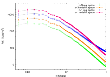
Figure 3: Power spectrum of the dark matter distribution at $z=3$ (lower curves) and $z=1$ (upper curves). The dashed lines are the linearly evolved initial power spectrum. In the case of redshift space, the linear power spectrum was multiplied in addition by $1+2/3\,\beta(z)+1/5\,\beta(z)^{2}\approx 1.843\,(1.714)$ for $z=3\,(1)$.

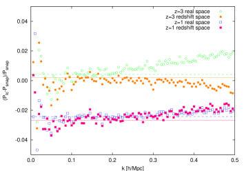
Figure 4: Fractional difference of the light-cone power spectrum $P_{\rm lc}$ and the power spectrum at the corresponding snapshot $P_{\rm snap}$. The horizontal lines show the predicted shifts from linear theory in real space (dashed) and redshift space (solid).

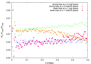
Figure 5: Fractional difference of the galaxy light-cone power spectrum $P_{\rm lc}$ and the galaxy power spectrum at the corresponding snapshot $P_{\rm snap}$.

In Fig. 3, we show the isotropic dark matter power spectra at redshift $z=3$ and $z=1$ obtained by assuming the correct cosmology with $w_{\rm ref}=-1$. If not stated otherwise, we always use as the reference cosmology the cosmology of the simulation, i.e. we assume that $w_{\rm ref}=-1$. The linear redshift distortion (Kaiser 1987) amplifies the power by $1+2/3\,\beta(z)+1/5\,\beta(z)^{2}$ with $\beta(z)=f(z)/b(z)$, where $f(z)$ is the linear growth rate and $b(z)$ the bias parameter. In the case of dark matter we have $b=1$. For scales shown, the nonlinear evolution is still mild. The deviations in the real-space power spectra from the linearly evolved initial power spectra (plotted as dashed lines) start around $k\sim 0.25h/{\rm Mpc}$ and $k\sim 0.15h/{\rm Mpc}$ for $z=3$ and $z=1$, respectively. The nonlinear redshift distortions (“finger of God” effects) in redshift space lead to a suppression of power on small scales, which almost balances the increase in power due to nonlinear clustering at $z=1$ (filled squares in Fig. 3). The BAO can be seen as tiny wiggles in the power spectrum. Their amplitudes are $\lesssim 5\%$ of $P(k)$.

We do not show the light-cone power spectra, since they lie almost exactly on the corresponding snapshot power spectra. The fractional differences in the power spectra derived from the light cone and the corresponding snapshot are instead plotted in Fig. 4. On linear scales, the fractional differences are $\sim 0.5\%$ and $\sim-2.5\%$ at $z=3$ and $z=1$, respectively. The reason for these differences is that the value of the growth function at the mean redshift is not equal to the mean growth function. The stated numbers can be understood by averaging the square of the redshift-dependent growth function multiplied by an appropriate geometrical factor over the survey box (Yamamoto et al. 1999). Numerical calculations for our survey designs are shown as dashed (real space) and solid (redshift space) lines. The deviations at larger $k$ are due to nonlinear effects. The question of whether these light-cone effects alter the fitting of the BAO is addressed in Sect. 5.

In Fig. 5, we compare the biased galaxy power spectra derived from the light cones with those evaluated for the corresponding snapshots. Qualitatively, we observe the same behavior as in the dark matter case. The larger scatter is due to higher shot noise and the means are shifted slightly, since, as happened before for the growth function, the bias at the mean redshift is not equal to the bias averaged over the appropriate redshift range.

4.2 Fitting procedure

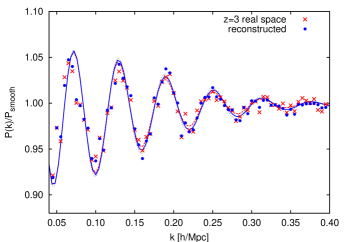
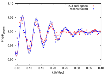
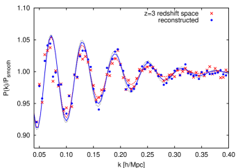
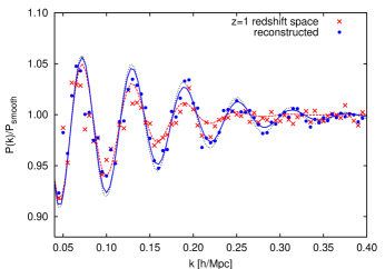
Figure 6: The left upper panel shows the oscillatory part of the power spectrum at redshift $z=3$ obtained from real space and its best-fit function including the suppression factor (dashed line). The dotted line corresponds to the oscillatory part of the initial power spectrum. The solid line is the best-fit of the reconstructed data. At the bottom left, we present the same in redshift space. On the right the corresponding plots for $z=1$ are shown.

Our fitting method attempts to remove all the information apart from the BAO themselves. This is easily achieved by dividing the power spectrum by a smoothed version of itself. The advantage of this is that one does not need to model all the physical processes that alter the power spectrum such as redshift distortion, nonlinear evolution, and galaxy bias or uncertainties in cosmological parameters, such as $\sigma_{8}$, $n_{s}$, and massive neutrinos, which affect the overall shape of the power spectrum but have little effect on the BAO.

The extracted BAO of the reference power spectra were then fitted to the extracted BAO, allowing the scaling factors $\lambda_{\parallel,\bot}$ or $\lambda_{\rm iso}$ to vary. In an additional fitting attempt, our free parameter is instead the EOS parameter $w$ and we derive the scaling factors $\lambda_{\parallel,\bot}$ or $\lambda_{\rm iso}$ by applying Eq. (5).

The fitting parameters are determined by Monte Carlo Markov chain (MCMC) techniques. We use the Metropolis-Hastings algorithm (Metropolis et al. 1953; Hastings 1970) to build up the Markov chain.

In the following, we describe each step of the fitting procedure.

Smoothing

There are previous proposals to use only the oscillatory part of the power spectrum for measuring the scale of the BAO (Blake & Glazebrook 2003; Glazebrook & Blake 2005; Hütsi 2005, 2006a; Koehler et al. 2007; Angulo et al. 2008; Percival et al. 2007b). All of them divide the power spectrum by (or subtract from it) a non-oscillating fit. The methods used to derive the smooth fit range from deriving a semi-analytic zero-baryon reference power spectrum, fitting with a quadratic polynomial in log-log space, or using a cubic spline, to fitting with a non-oscillating phenomenological function. In this paper, we generate a smoothed power spectrum in an almost parameter-free way, by computing for each point the arithmetic mean in log space of its neighbors in a range of $\pm 0.03\,h/\rm{Mpc}$ in $k$. In the two-dimensional case, we smooth radially in the direction of $|k|$. This smoothing length is the only parameter in our smoothing method, which, for all input power spectra, we select to have the same value of approximately equal to the wavelength of the BAO.

By dividing the measured power spectrum by its smoothed version, we derive the purely oscillatory part of the power spectrum $P_{\rm{osci}}=P/P_{\rm{smooth}}$ (see Fig. 6).

Fitting and Priors

In place of fitting the extracted BAO by a (modified) sine function (Blake & Glazebrook 2003; Glazebrook & Blake 2005) or using a periodogram (Hütsi 2005) to measure the scale of the BAO, we compare the BAO with a range of different oscillatory reference power spectra $P_{\rm osci}^{\rm ref}$ produced from thousands of linear power spectra generated with CMBfast, which differ in the cosmological parameters $\Omega_{\rm m}$, $\Omega_{\rm b}$, $H_{\rm 0}$, and $n_{\rm s}$.

We prefer this method since the BAO are not exactly harmonic (Eisenstein & Hu 1998; Koehler et al. 2007) and the uncertainties in the aforementioned cosmological parameters can easily be included. As priors on these cosmological parameters we use the predicted uncertainties for the Planck mission (The Planck Bluebook 2005). For the Hubble constant $H_{0}$, we combine the Planck priors with constraints provided by large-scale structure (Percival et al. 2007a) and include measurements from the HST Key project (Freedman et al. 2001):

$$\begin{aligned} \Delta\omega_{\rm m}&=1.25\%\ ,\ \ \Delta H_{\rm 0}=5\%\ ,\\ \Delta\omega_{\rm b}&=0.75\%\ ,\ \ \Delta n_{\rm s}=0.5\%\ ,\end{aligned}$$ (10)

where $\omega_{\rm m}=\Omega_{\rm m}\,h^{2}$ and $\omega_{\rm b}=\Omega_{\rm b}\,h^{2}$. We assume throughout this article that the Universe is spatially flat.

We determine the scaling factors $\lambda_{\parallel,\bot}$ or $\lambda_{\rm iso}$ by fitting a scaled $P_{\rm osci}^{\rm ref}(\lambda_{\parallel}k_{\parallel},\lambda_{\bot}k_{\bot})$ or $P_{\rm osci}^{\rm ref}(\lambda_{\rm iso}k)$ to $P_{\rm{osci}}$.

Damping and Reconstruction

Since nonlinear structure growth diminishes the amplitudes of the wiggles (Eisenstein et al. 2007b), we can improve the fitting by adding a suppression factor $W=\exp(-\sigma k^{2})$ to our fitting function

$$P_{\rm osci}(k)=W\left[P_{\rm osci}^{\rm ref}(\lambda_{\rm iso}k)-1\right]+1\,.$$ (11)

For the two-dimensional redshift-space power spectrum, we have to introduce two suppression parameters $\sigma_{\parallel,\bot}$, since the redshift space distortion increases suppression along the line of sight. The suppression factor then becomes $W=\exp(-\sigma_{\parallel}k_{\parallel}^{2}-\sigma_{\bot}k_{\bot}^{2})$.

If the density field is known accurately, i.e. the shot noise is small and the galaxy bias is known, it is possible to use reconstruction techniques (see e.g. Narayanan & Croft (1999) for a comparison of methods) to undo, at least in part, the suppression of the wiggles (Eisenstein et al. 2007a). We applied the PIZA method (Croft & Gaztanaga 1997) to the dark matter distributions. We attempted a similar technique for the mock catalogs but due to shot noise and galaxy bias our results were unsatisfactory. Further efforts are required to achieve this goal. In Fig. 6, we indicate the BAO extracted from the data by crosses. The dashed lines show the best-fit functions and the dotted lines depict the corresponding non-damped reference $P_{\rm osci}^{\rm ref}(k)$. We observe that the suppression of the BAO is higher in redshift space and increases with time. Additionally, the results of the reconstructed density fields are plotted (data as filled circles and the best-fits as solid lines). The amplitude of the BAO could not be reestablished completely but to a significant fraction.

Fitting Range

The $k$ range over which we use the data for our fitting plays an important role. In the fitting procedure we use a minimum wave number $k_{\rm min}=0.04\,h/{\rm Mpc}$, since for the points with $k<0.03\,h/{\rm Mpc}$ the smoothing is not well defined, and the error due to sample variance is high. As the maximum wave number, we select $k_{\rm max}=0.25\,(0.30)$, for redshift $z=1\,(3)$. Although nonlinear evolution has already started on these scales, the BAO are still clearly visible (see Fig. 6).

5 Results

The most important measurements in our analysis are the marginalized probability distribution functions (PDF) of the scaling factors and the EOS parameter $w$. To determine their values, we marginalize the joint PDF produced via the MCMC technique over all other fitting parameters. From these functions, we can derive the best-fit values and the accuracy of both the scaling factors and the EOS $w$.

Fitting method, real space versus redshift space, and degeneracies

With the twelve $256^{3}$ simulations we assess the robustness of our fitting method and the presence of systematic effects. We determine the best-fitting scaling factors, both parallel and transverse to the line of sight, for the dark matter power spectrum in real and redshift space for all twelve simulations at redshift $z=10$, $3$, and $1$. For all redshifts, we find that the mean value of the twelve simulations is clearly less than $1\sigma$ (standard deviation) away from unity. Hence, our fitting method provides unbiased results within the margins of error (see Table 1).

Table 1: Results for the scaling factors $\lambda_{\parallel}$ and $\lambda_{\bot}$ obtained from the dozen $256^{3}$ simulations.

	Real Space		Redshift Space		Difference
Parameter	mean	sigma	mean	sigma	mean	sigma
$z=10$
$\lambda_{||}$	$0.998$	$0.007$	$0.998$	$0.008$	$\phantom{-}0.000$	$0.001$
$\lambda_{\bot}$	$0.999$	$0.005$	$0.999$	$0.005$	$\phantom{-}0.000$	$0.001$
$z=3$
$\lambda_{||}$	$0.998$	$0.009$	$0.999$	$0.011$	$-0.002$	$0.004$
$\lambda_{\bot}$	$1.000$	$0.006$	$0.999$	$0.006$	$\phantom{-}0.001$	$0.002$
$z=1$
$\lambda_{||}$	$0.997$	$0.010$	$0.999$	$0.014$	$-0.003$	$0.008$
$\lambda_{\bot}$	$0.999$	$0.009$	$0.999$	$0.010$	$\phantom{-}0.000$	$0.003$

The differences between results for real and redshift space in each simulation do not show a systematic trend. The mean difference is in fact consistent with zero. The error in the scale factor parallel to the line of sight $\lambda_{||}$ is larger in redshift space, since the damping of the BAO is stronger in redshift space (see Fig 6).

To understand the degeneracies in the scaling factor for the cosmological parameters included in our method, we complete the fitting by keeping all cosmological parameters fixed to the value of the simulation apart from the parameter under consideration, for which we calculate the PDF of $\lambda_{\rm iso}$ for different values of this parameter. The corresponding $95\%$ confidence lines for the dark matter power spectrum at $z=3$ (solid) and at $z=1$ (dotted) are shown in Fig. 7. Since the sound horizon imprinted in the power spectrum is redshift independent, we expect that the derived degeneracies are also redshift independent. This is indeed the case for our fitting method. The only difference with respect to $z$ is the larger uncertainty in $\lambda_{\rm iso}$ at lower redshifts due to the suppression of the BAO by nonlinear evolution.

The interval of cosmological parameters plotted in Fig. 7 was chosen to be centered on the values of the simulation and in the range of $\pm 3\%$. In this way, we can immediately assess the degree of degeneracy. We find that if we alter one of the cosmological parameters by $1\%$ the scaling factor changes by $0.22\%$ for $\omega_{\rm m}$, $0.14\%$ for $\omega_{\rm b}$, $\sim 0\%$ for $H_{0}$, and $0\%$ for $n_{\rm s}$. These numbers agree well with those given by the fitting formula for the sound horizon by Eisenstein & Hu (1998):

$$s=\frac{44.5\,{\ln}(9.83/\omega_{\rm m})}{\sqrt{1+10\,\omega_{\rm b}^{3/4}}}\,\rm Mpc\,.$$ (12)

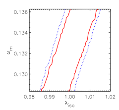
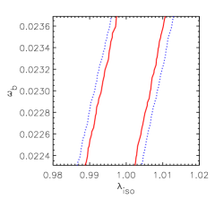
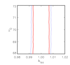
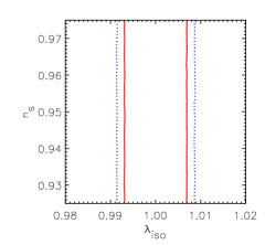
Figure 7: Dependence of the fitted $\lambda_{\rm iso}$ on the cosmological parameters $\omega_{\rm m}$, $\omega_{\rm b}$, $H_{0}$, and $n_{\rm s}$ at redshift $z=3$ (solid) and $z=1$ (dotted).

More interesting are the dependences of the equation of state $w$ on the cosmological parameters, in particular the dependence on $\omega_{\rm m}$ and $H_{0}$, which enter the relation between the scaling factors and $w$. For a constant $w$ model ($w=w_{0}$), we indicate the derived correlations in Fig. 8, where the solid line corresponds to $z=3$ and the dotted line to $z=1$. In contrast to the previous case, these correlations are redshift dependent, for example at $z=1$ the dependence of both the sound horizon and the Hubble parameter $H(z)$ on $\omega_{\rm m}$ almost exactly cancel each other, whereas at $z=3$ the effect originating in the Hubble parameter $H(z)$ is stronger. Among the cosmological parameters the largest uncertainty in $w_{0}$ originates in $H_{0}$, in particular at lower redshifts.

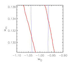
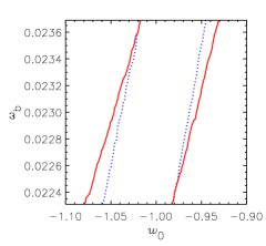
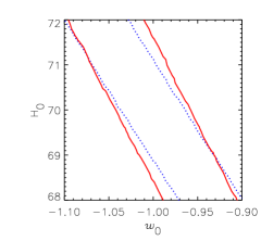
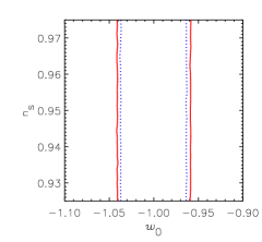
Figure 8: Same as in Fig. 7 but for $w_{0}$.

Light-cone effect

We have already mentioned that the power spectra derived from the light cone output and corresponding snapshot at the mean redshift are almost on top of each other. The more evolved parts of the light-cone sample compensate almost precisely the less evolved parts, such that its power spectrum is almost identical to that at the mean redshift (see Fig. 4). In Fig. 9 we show the corresponding PDFs of the scaling factors. The lines show the $68\%$ and $95\%$ confidence levels obtained from the dark matter snapshot (dashed) and light-cone (dotted) power spectra at redshift $z=3$ (left) and $z=1$ (right) in real (top) and redshift space (bottom). The differences in the error ellipses derived from the light-cone and snapshot data are overall small. Hence, light-cone effects in this survey volume and at these redshifts are unimportant to our fitting.

Reconstruction

The error ellipses for the reconstructed samples are shown in Fig. 9 as solid lines. We observe that for data at $z=1$ in redshift space the reconstruction of the BAO shrinks the error ellipses by a factor of three. For this reason, it would be desirable to develop a reconstruction method that can be applied to noisy and biased density fields. For surveys at redshift $z=3$, this effect is less important.

Orientation of the error ellipse

The errors in the scaling factors originate in two different sources. One source is the errors in the power spectrum; the other source is the uncertainties in the cosmological parameters $\omega_{\rm m}$ and $\omega_{\rm b}$, which produce an uncertainty in the sound horizon, i.e. the scale of the BAO. If the principal error could be attributed to the uncertainty in the physical sound horizon, the orientation of the ellipse would be approximately in the direction of the line defined by $\lambda_{\bot}=\lambda_{||}$. For a low signal-to-noise ratio power spectrum for which the scale of the BAO in the power spectrum cannot be determined accurately, the orientation of the error ellipse is instead in the direction of the line of $\sqrt[3]{\lambda_{\bot}^{2}\lambda_{||}}=\rm const$.

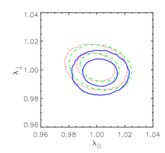
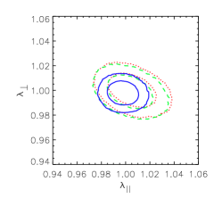
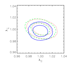
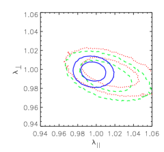
Figure 9: The marginalized probability distribution functions (PDF) of the scaling factors at redshifts $z=3$ (left) and $z=1$ (right) in real space (top) and redshift space (bottom) derived from the light cone (dotted), snapshot (dashed), and “reconstructed” light cone (solid).

Cosmological distortion

We assess if the approximations to compensate for an incorrect reference cosmology i.e. the scaling relations given in Eq. (4), are sufficiently accurate for our simulated surveys. We calculate the distances assuming three reference cosmologies that differ only in terms of $w_{\rm ref}$ and compute the corresponding power spectra.

As an example, the oscillatory parts of the dark matter power spectra at $z=3$ in real space are shown in Fig. 10. We observe that the scale of the oscillations is compressed and stretched for $w_{\rm ref}=-1.2$ and $w_{\rm ref}=-0.8$, respectively.

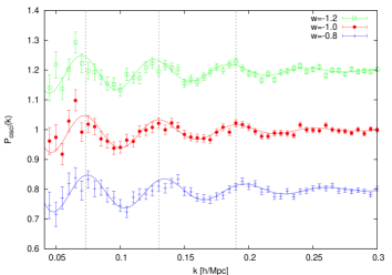
Figure 10: The oscillatory part of the real space power spectra at redshift $z=3$ derived for three different cosmologies and its best-fit function. For display purposes, the power spectrum for $w_{\rm ref}=-1.2(-0.8)$ is shifted $+0.2(-0.2)$ along the $y$-axis.

We scale the one-dimensional power spectra according to the scaling relation, i.e. $P(k)\rightarrow\lambda_{\rm iso}^{3}\,P(k/\lambda_{\rm iso})$, where the factor $\lambda_{\rm iso}^{3}$ is due to the scaled volume element. The fractional difference of these scaled power spectra with respect to that of the correct cosmology, i.e. $w=-1$, is shown in Fig. 11. The data points for $w=-1.2$ (squares) and $w=-0.8$ (plus signs) are shifted by $+0.25\%$ and $-0.40\%$, respectively, to center them on the zero line. These small shifts have a similar origin as in the light-cone versus snapshot comparison; we calculate the scaling factor at the mean redshift, which is not equal to the mean scaling factor. The noise in the scaled power spectra is substantially smaller on large scales than the error, which is already implicit in the power spectrum due to cosmic variance (dashed line) and additional shot noise (solid line). To determine if this (additional) noise impairs the fitting of the BAO and with it the measurement of the equation of state $w$, we fit the corresponding data of the twelve $256^{3}$ simulations by assuming a constant $w$. We find that the best-fit value for $w_{0}$ varies among the different reference cosmologies for a single simulation by not more than $4\%$, and is typically $\sim 2\%$. This should be compared with the standard deviation for a single $w_{0}$ measurement, which is about $3\%$. All PDFs scatter about the mean value of $w_{0}=-1$, no systematic effects are noticeable. We conclude that the scaling relations do not introduce a noticeable bias or enlarge the error in $w$. For real data, a consistency check would be to recalculate the distances and corresponding power spectrum and redo the analysis using the measured $w$ as the reference value for the assumed cosmology.

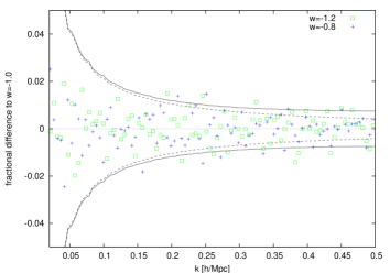
Figure 11: The fractional difference of the scaled real-space power spectra at redshift $z=3$ is shown for the three different reference cosmologies. Note that the data points for $w=-1.2$ and $w=-0.8$ are shifted vertically by $+0.0025$ and $-0.0040$, respectively, to enhance the visibility of the scatter. The lines show the intrinsic error in the power spectrum due to cosmic variance (dashed line) plus shot noise (solid line).

Constraining $w$ with the (an)isotropic power spectrum

The two-dimensional power spectrum provides the possibility to measure $\lambda_{\parallel}$ and $\lambda_{\bot}$, instead of the combination $\lambda_{\rm iso}$ only, as in the case of the one-dimensional power spectrum. Since both scaling factors depend on $w$ in different ways, we expect that $w$ is more accurately constrained by the two-dimensional power spectrum. In the case of a simple constant $w$, this is not the case: both the mean values and the errors are similar to those derived from the one-dimensional power spectra. For more complex models of $w$, the measurement of $\lambda_{\parallel}$ and $\lambda_{\bot}$ is very helpful as we see from Fig. 12, where we applied the model $w=w_{0}+(1-a)w_{a}$. For display purposes, we performed a coordinate transformation of the parameters to the “pivot” system $w_{0}+(1-a)w_{a}=w_{\rm p}+(a_{\rm p}-a)w_{a}$ where we chose $z_{\rm p}=0.3$ as discussed below. The left (right) panel indicates the constraints obtained from the dark matter light-cone power spectrum around $z=3$ ($z=1$) in real space. One sees that for $z=3$ the contour lines are open towards negative $w_{a}$ even for the two-dimensional case. Nevertheless, in both redshift cases the use of the anisotropic power spectrum tightens the constraints substantially.

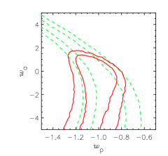
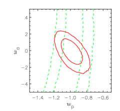
Figure 12: This plot shows the $68\%$ and $95\%$ confidence levels for the redshift-dependent $w$ model obtained from the one-dimensional (dashed lines) and two-dimensional (solid lines) dark matter power spectrum at redshift $z=3$ (left) and $z=1$ (right) in real space.

Estimates for future surveys

For a prediction of how well upcoming observations will enable $w$ to be measured, we analyze the mock galaxy catalogs introduced above, namely the weakly and strongly biased one million galaxy catalogs at redshift $z=3$ and the one and two million galaxy catalogs at $z=1$. In Fig. 13, we present typical fitting results of the scaling factors for each type of catalogs. For the solid lines, we used the aforementioned priors on the cosmological parameters, whereas for the dashed lines we fixed these parameters.

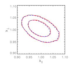
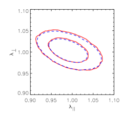
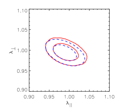
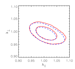
Figure 13: Typical contour plots of the joint PDF of $\lambda_{\parallel}$ and $\lambda_{\bot}$ obtained from the mock catalogs at redshift $z=3$ (left: weak (top) and strong (bottom) bias) and $z=1$ (right: 1 million (top) and 2 million (bottom) galaxies) are shown. The contour lines correspond to 68% and 95% confidence level. The dashed line shows the results when the cosmological parameters are fixed at the values of the simulation.

Since the error in the scaling factors is dominated by the errors in the power spectrum, improving the accuracy of the cosmological parameters to higher than that of the assumed priors does not significantly reduce the error in the scaling factors. However, it tightens the constraints on $w$ (see Fig. 14 for constant $w$): the uncertainty in $H_{0}$, in particular, degrades the measurement of $w$.

For the strongly biased sample at $z=3$ of one million galaxies in a volume of $10\,{\rm Gpc}^{3}$, the mean uncertainties in the Hubble parameter ($H(z)\varpropto\lambda_{\parallel})$ and angular diameter distance ($D_{A}(z)\varpropto 1/\lambda_{\bot}$) are $1.8\%$ and $1.2\%$ ($68\%$ c.l.), respectively. This corresponds to an error of $\sim 12\%$ for a constant $w$. By keeping the cosmological parameters fixed, the uncertainty in $w$ is lowered to $\sim 5\%$.

The corresponding numbers for the two million galaxy mock catalog at $z=1$ are $2.8\%$ and $1.6\%$ for the Hubble parameter and angular diameter distance, respectively. In this case, we derive an accuracy of $\sim 11\%$ and $\sim 4\%$ for a constant $w$ with Planck priors and fixed cosmology, respectively.

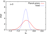
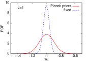
Figure 14: PDFs for constant $w$ derived from the one million strongly biased galaxy sample at $z=3$ (left) and from the two million galaxy at $z=1$ (right).

To translate the results for the scaling factors into constraints of the redshift-dependent $w$-model $w=w_{0}+(1-a)w_{a}$, we combine the data of the strongly biased one million galaxy catalog at $z=3$ and two million galaxy catalog at $z=1$ with 192 SN Ia observations (Davis et al. 2007; Wood-Vasey et al. 2007; Riess et al. 2007; Astier et al. 2006). In addition we include constraints from CMB measurements by holding the ratio of the distance to the last scattering surface and the sound horizon fixed: $D_{A}(z=z_{\rm lss})/s=\rm const$.

The confidence contours for $w_{0}$ and $w_{a}$ are shown in the upper panels of Fig. 15. In the lower panels, the confidence contours are presented in the pivot variable $w_{\rm p}=w_{0}+(1-a_{\rm p})w_{a}$, where we choose $a_{\rm p}$ such that the error “ellipse” from the combined datasets (solid line) is least tilted; we find $a_{\rm p}=1/(1+0.3)$. One sees that the intersection angle of the BAO contours with respect to the error ellipse derived from SN data varies with redshift (see also Fig. 16). For $z=3$, the orientation is very similar to the CMB contours, whereas for $z=1$, it is more aligned with the SN ellipse. Measurements at both redshifts would therefore constrain the parameters of this model significantly more than two (or twice a good) measurements at a single redshift.

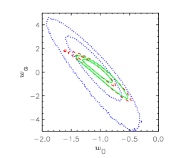
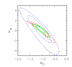
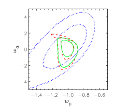
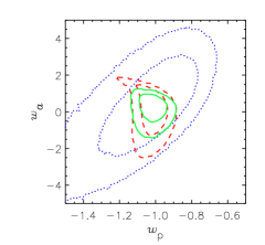
Figure 15: The $68\%$ and $95\%$ confidence level for the parameters of the model $w=w_{0}+(1-a)w_{a}$ obtained from SN (dotted), SN+CMB (dashed), and SN+CMB+BAO (solid). Results for the strongly biased one million galaxy sample are shown at $z=3$ (left) and for the weakly biased two million galaxy sample at $z=1$ (right). At the bottom, we show the same results but transformed to the pivot system $z_{\rm p}=0.3$.

In Fig. 16, we show the constraints on $w$ derived alone from BAO measurements at two different redshifts, namely $z=1$ (dashed lines) and $z=3$ (dotted lines), and the combination of both measurements (solid lines). The redshift-dependent shape and orientation of the contour lines is clearly evident in the pivot system (right panel).

For all confidence contours in Fig. 15 and Fig. 16, the above stated priors for the cosmological parameters $\omega_{\rm m}$, $\omega_{\rm b}$, $n_{\rm s}$, and $H_{0}$ were used.

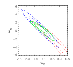
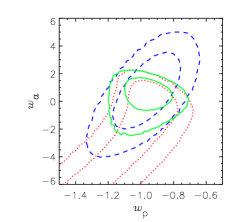
Figure 16: The $68\%$ and $95\%$ confidence level for the parameters of the model $w=w_{0}+(1-a)w_{a}$ obtained from the BAO measurements in the strongly biased one million galaxy sample at $z=3$ (dotted) and in the weakly biased two million galaxy sample at $z=1$ (dashed). The solid lines show the combination of both BAO measurements. On the right, the contours are transformed to the pivot system of the combined dataset $a_{\rm p}=0.7$.

6 Discussion and Conclusions

We have simulated large redshift surveys by “observing” mock galaxies on a light cone obtained from an N-body simulation with $512^{3}$ dark matter particles in a $(1.5\,{{\rm Gpc}/h})^{3}$ box. By fitting the apparent scale of the BAO in the power spectrum, we have derived constraints on the EOS parameter $w$.

Our fitting method uses only the oscillatory part of the power spectrum and is therefore insensitive to changes in the power spectrum due to nonlinear evolution, redshift distortions, and scale-dependent galaxy bias. Fitting methods that use the overall shape of the power spectrum suffer in general from these complicated physical effects (unless they are accurately modeled) and tend to provide biased results (Smith et al. 2008).

The drawback of fitting only the oscillatory part is that it is insensitive to information provided by the overall shape of the power spectrum. Determining the growth function would be interesting in particular for dark energy constraints (Amendola et al. 2005; Sapone & Amendola 2007).

It is unclear how to extract the BAO from the power spectrum in the most appropriate and accurate way. Our simple smoothing method works fairly well. It is essentially parameter-free and produces unbiased and robust results.

We analyzed the degeneracies in the EOS $w$ with other cosmological parameters. Given the expected accuracies in the cosmological parameters involved, we found that more accurate measurements of $H_{0}$ would have the largest effect on lowering the uncertainties in $w$, especially for observations at lower redshifts.

Comparing the results of the light-cone power spectrum with those of the power spectrum of the snapshot at the corresponding redshift, we did not find evidence for substantial differences. For the surveys under consideration, light cone effects therefore do not play a role in determining $w$ with our fitting method. This is in addition true, when we include redshift-dependent galaxy bias. Fitting methods, sensitive to the overall shape of the power spectrum, in particular to the growth function, must include explicitly the light-cone effects to produce unbiased results.

The PIZA technique (Croft & Gaztanaga 1997), which is used to reconstruct the linear density field and thereby the amplitude of the BAO, is effective if the density field is known to sufficient accuracy. In the case of substantial shot noise and unknown galaxy bias, more sophisticated reconstruction techniques are required.

To investigate the cosmological distortion due to an incorrect reference cosmology, we adopted three different reference cosmologies with different values for $w_{\rm ref}=-0.8$, $-1.0$, and $-1.2$. Employing the usual scaling relations (see Eq. (5)), we found in all three cases similar fitting results within the margins of error. We conclude that even for this large survey volume the simple scaling of the power spectrum is fairly accurate. Nevertheless, for real data we propose to use an iterative scheme; after measuring $w$ for an assumed reference cosmology, one would then repeat the analysis for the updated reference cosmology, using the measured value of $w$ for $w_{\rm ref}$.

By fitting the two-dimensional power spectrum, we can determine independently both scaling factors. For a constant $w$, the two-dimensional fitting does not improve the constraints on $w$ significantly. For models of $w$ that are not so tightly constrained, independent measurements of the Hubble parameter ($H(z)\varpropto\lambda_{\parallel})$ and the angular diameter distance ($D_{A}\varpropto 1/\lambda_{\bot}$) will however be very helpful. For the model $w=w_{0}+(1-a)w_{a}$, this is especially true at lower redshifts.

Our estimates for future surveys show that BAO measurements around redshifts $z=3$ and $z=1$ in combination with SN and CMB data tighten the constraints on dynamical dark energy substantially and that these redshift surveys deliver complementary results. For a constant $w$-model the BAO measurements from our two mock catalogs at $z=3$ and $z=1$ alone will constrain $w_{0}$ to an accuracy of $\sim 12\%$ and $\sim 11\%$, respectively.

To achieve more realistic predictions, the survey geometry, i.e. the window function, has to be taken into account. A more realistic galaxy bias scheme, tailored in particular for the target galaxies, should also be developed. For such a study, large-volume simulations of far higher mass resolution are needed.

References

- Albrecht et al. (2006) Albrecht, A., Bernstein, G., Cahn, R., et al. 2006, arXiv:astro-ph/0609591
- Amendola et al. (2005) Amendola, L., Quercellini, C., & Giallongo, E. 2005, Mon. Not. Roy. Astron. Soc., 357, 429
- Angulo et al. (2005) Angulo, R., Baugh, C. M., Frenk, C. S., et al. 2005, MNRAS, 362, L25
- Angulo et al. (2008) Angulo, R. E., Baugh, C. M., Frenk, C. S., & Lacey, C. G. 2008, MNRAS, 383, 755
- Astier et al. (2006) Astier, P. et al. 2006, Astron. Astrophys., 447, 31
- Bassett et al. (2005) Bassett, B. A., Nichol, B., & Eisenstein, D. J. 2005, Astronomy and Geophysics, 46, 26
- Blake & Glazebrook (2003) Blake, C. & Glazebrook, K. 2003, ApJ, 594, 665
- Blake et al. (2006) Blake, C., Parkinson, D., Bassett, B., et al. 2006, MNRAS, 365, 255
- Bond & Efstathiou (1984) Bond, J. R. & Efstathiou, G. 1984, ApJ, 285, L45
- Carroll (2001) Carroll, S. M. 2001, Living Reviews in Relativity, 4, 1
- Cole et al. (1998) Cole, S., Hatton, S., Weinberg, D. H., & Frenk, C. S. 1998, Mon. Not. Roy. Astron. Soc., 300, 945C
- Cole et al. (2005) Cole, S., Percival, W. J., Peacock, J. A., et al. 2005, MNRAS, 362, 505
- Croft & Gaztanaga (1997) Croft, R. A. C. & Gaztanaga, E. 1997, MNRAS, 285, 793
- Davis et al. (2007) Davis, T. M., Mörtsell, E., Sollerman, J., et al. 2007, ApJ, 666, 716
- Eisenstein & Hu (1998) Eisenstein, D. J. & Hu, W. 1998, ApJ, 496, 605
- Eisenstein et al. (1998) Eisenstein, D. J., Hu, W., & Tegmark, M. 1998, ApJ, 504, L57
- Eisenstein et al. (1999) Eisenstein, D. J., Hu, W., & Tegmark, M. 1999, ApJ, 518, 2
- Eisenstein et al. (2007a) Eisenstein, D. J., Seo, H.-J., Sirko, E., & Spergel, D. N. 2007a, ApJ, 664, 675
- Eisenstein et al. (2007b) Eisenstein, D. J., Seo, H.-J., & White, M. 2007b, ApJ, 664, 660
- Eisenstein et al. (2005) Eisenstein, D. J., Zehavi, I., Hogg, D. W., et al. 2005, ApJ, 633, 560
- Evrard et al. (2002) Evrard, A. E., MacFarland, T. J., Couchman, H. M. P., et al. 2002, ApJ, 573, 7
- Feldman et al. (1994) Feldman, H. A., Kaiser, N., & Peacock, J. A. 1994, ApJ, 426, 23
- Freedman et al. (2001) Freedman, W. L., Madore, B. F., Gibson, B. K., et al. 2001, ApJ, 553, 47
- Gawiser et al. (2007) Gawiser, E., Francke, H., Lai, K., et al. 2007, ApJ, 671, 278
- Glazebrook & Blake (2005) Glazebrook, K. & Blake, C. 2005, ApJ, 631, 1
- Glazebrook et al. (2005) Glazebrook, K., Eisenstein, D., Dey, A., Nichol, B., & The WFMOS Feasibility Study Dark Energy Team. 2005, arXiv:astro-ph/0507457
- Gottlöber et al. (2006) Gottlöber, S., Yepes, G., Wagner, C., & Sevilla, R. 2006, in From Dark Halo to Light, ed. S. Maurogordato, J. Tran Thanh Van, & L. Tresse, Proc. XLI Moriond (Gioi publishers), 309
- Gronwall et al. (2007) Gronwall, C., Ciardullo, R., Hickey, T., et al. 2007, ApJ, 667, 79
- Hastings (1970) Hastings, W. 1970, Biometrika, 57, 97
- Hill et al. (2004) Hill, G. J., Gebhardt, K., Komatsu, E., & MacQueen, P. J. 2004, AIP Conf. Proc., 743, 224
- Hockney & Eastwood (1988) Hockney, R. W. & Eastwood, J. W. 1988, Computer simulation using particles (Bristol: Hilger, 1988)
- Holtzman (1989) Holtzman, J. A. 1989, ApJS, 71, 1
- Hu & Haiman (2003) Hu, W. & Haiman, Z. 2003, Phys. Rev. D, 68, 063004
- Hu & Sugiyama (1996) Hu, W. & Sugiyama, N. 1996, ApJ, 471, 542
- Huff et al. (2007) Huff, E., Schulz, A. E., White, M., Schlegel, D. J., & Warren, M. S. 2007, Astroparticle Physics, 26, 351
- Hütsi (2005) Hütsi, G. 2005, arXiv:astro-ph/0507678
- Hütsi (2006a) Hütsi, G. 2006a, A&A, 449, 891
- Hütsi (2006b) Hütsi, G. 2006b, A&A, 446, 43
- Hütsi (2006c) Hütsi, G. 2006c, A&A, 459, 375
- Jing (2005) Jing, Y. P. 2005, ApJ, 620, 559
- Kaiser (1987) Kaiser, N. 1987, MNRAS, 227, 1
- Koehler et al. (2007) Koehler, R. S., Schuecker, P., & Gebhardt, K. 2007, A&A, 462, 7
- Linder (2003) Linder, E. V. 2003, Phys. Rev. D, 68, 083504
- Linder (2007) Linder, E. V. 2007, arXiv:0708.0024
- Matsubara (2004) Matsubara, T. 2004, ApJ, 615, 573
- Metropolis et al. (1953) Metropolis, N., Rosenbluth, A., Rosenbluth, M., Teller, A., & Teller, E. 1953, J. Chem. Phys., 21, 1087
- Narayanan & Croft (1999) Narayanan, V. K. & Croft, R. A. C. 1999, ApJ, 515, 471
- Peebles & Yu (1970) Peebles, P. J. E. & Yu, J. T. 1970, ApJ, 162, 815
- Percival et al. (2007a) Percival, W. J. et al. 2007a, Mon. Not. Roy. Astron. Soc., 381, 1053
- Percival et al. (2007b) Percival, W. J. et al. 2007b, Astrophys. J., 657, 51
- Perlmutter et al. (1999) Perlmutter, S., Aldering, G., Goldhaber, G., et al. 1999, ApJ, 517, 565
- Riess et al. (1998) Riess, A. G., Filippenko, A. V., Challis, P., et al. 1998, AJ, 116, 1009
- Riess et al. (2007) Riess, A. G., Strolger, L.-G., Casertano, S., et al. 2007, ApJ, 659, 98
- Sapone & Amendola (2007) Sapone, D. & Amendola, L. 2007, arXiv:07092792
- SDSS-III Collaboration (2008) SDSS-III Collaboration. 2008, http://www.sdss3.org/cosmology.php
- Seljak & Zaldarriaga (1996) Seljak, U. & Zaldarriaga, M. 1996, ApJ, 469, 437
- Seo & Eisenstein (2003) Seo, H.-J. & Eisenstein, D. J. 2003, ApJ, 598, 720
- Seo & Eisenstein (2005) Seo, H.-J. & Eisenstein, D. J. 2005, ApJ, 633, 575
- Seo & Eisenstein (2007) Seo, H.-J. & Eisenstein, D. J. 2007, ApJ, 665, 14
- Sirko (2005) Sirko, E. 2005, Astrophys. J., 634, 728
- Smith et al. (2008) Smith, R. E., Scoccimarro, R., & Sheth, R. K. 2008, Phys. Rev. D, 77, 043525
- Spergel et al. (2007) Spergel, D. N., Bean, R., Doré, O., et al. 2007, ApJS, 170, 377
- Spergel et al. (2003) Spergel, D. N., Verde, L., Peiris, H. V., et al. 2003, ApJS, 148, 175
- Springel (2005) Springel, V. 2005, MNRAS, 364, 1105
- Springel et al. (2005) Springel, V., White, S. D. M., Jenkins, A., et al. 2005, Nature, 435, 629
- Sunyaev & Zeldovich (1970) Sunyaev, R. A. & Zeldovich, Y. B. 1970, Ap&SS, 7, 3
- The KAOS Purple Book (2003) The KAOS Purple Book. 2003, http://www.noao.edu/kaos/KAOS_Final.pdf
- The Planck Bluebook (2005) The Planck Bluebook. 2005, http://www.rssd.esa.int/SA/PLANCK/docs/ Bluebook-ESA-SCI%282005%291_V2.pdf
- White (2005) White, M. 2005, Astroparticle Physics, 24, 334
- Wood-Vasey et al. (2007) Wood-Vasey, W. M., Miknaitis, G., Stubbs, C. W., et al. 2007, ApJ, 666, 694
- Yamamoto et al. (1999) Yamamoto, K., Nishioka, H., & Suto, Y. 1999, ApJ, 527, 488
- Yoshida et al. (2001) Yoshida, N. et al. 2001, Mon. Not. Roy. Astron. Soc., 325, 803