Pairing-based cooling of Fermi gases

Abstract

We propose a pairing-based method for cooling an atomic Fermi gas. A three component (labels 1, 2, 3) mixture of Fermions is considered where the components 1 and 2 interact and, for instance, form pairs whereas the component 3 is in the normal state. For cooling, the components 2 and 3 are coupled by an electromagnetic field. Since the quasiparticle distributions in the paired and in the normal states are different, the coupling leads to cooling of the normal state even when initially $T_{paired}\geq T_{normal}$. The cooling efficiency is given by the pairing energy and by the linewidth of the coupling field. No superfluidity is required. The method has a conceptual analogy to cooling based on superconductor – normal metal (SN) tunneling junctions. Main differences arise from the exact momentum conservation in the case of the field-matter coupling vs. non-conservation of momentum in the solid state tunneling process. Moreover, the role of processes that relax the energy conservation requirement in the tunneling, e.g. thermal fluctuations of an external reservoir, is now played by the linewidth of the field. The proposed method should be experimentally feasible due to its close connection to RF-spectroscopy of ultracold gases which is already in use.

Figure 1: (Color online) The normal state can be cooled by filling thermal holes (a) or removing hot particles (b). Net cooling is achieved because the thermal quasiparticle distributions are different in the (N) normal and (S) paired (energy (pseudo)gap $\Delta$) states. The picture is schematic: there is no spatial tunneling barrier, instead, the normal and paired states are coupled by an electromagnetic field.

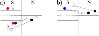
Cooling is often a prerequisite for observing correlated quantum states of matter, as has been demonstrated, e.g., by the history of superconductivity, superfluidity and the quantum Hall effect. In the case of ultracold atoms, laser cooling and evaporative cooling have enabled the observation of Bose-Einstein condensates Anderson et al. (1995); Davis et al. (1995), Mott insulator states Greiner et al. (2002) and condensates of strongly interacting Fermi gases Jochim et al. (2003); Regal et al. (2003, 2004); Zwierlein et al. (2004); Bartenstein et al. (2004); Kinast et al. (2004); Chin et al. (2004); Zwierlein et al. (2005). The research is rapidly expanding to new directions such as search for novel quantum states in optical lattices, p-wave pairing, and studies of multi-component mixtures of Fermions. To reach the required temperatures also in these new systems, cooling that goes beyond the presently available methods may become necessary. We propose a method for cooling fermionic atoms in a normal state by an internal tunneling contact to a paired state. The coexisting paired and normal states can be realized by trapping a three-component Fermi gas and tuning the various inter-component couplings by Feshbach resonances. The effective tunneling contact is realized by coupling the internal states of the atoms by electromagnetic fields. The cooling method is closely related to RF-spectroscopy of the pairing gap in ultracold Fermi gases Chin et al. (2004); Kinnunen et al. (2004) and has an analogy to on-chip cooling methods of solid state structures via superconductor – normal metal (SN) tunneling junctions Giazotto et al. (2006).

The basic principle of the proposed cooling is illustrated in Fig. 1. A three-component Fermi gas is confined to a certain spatial volume, e.g. by an (optical) trap or lattice. Components 1 and 2 interact, for instance via a Feshbach resonance, whereas the component 3 does not interact with the other components. Components 2 and 3 are coupled by an electromagnetic field, with a certain (effective) detuning $\delta=\omega_{field}-\omega_{23}$ and Rabi frequency $\Omega$. All atoms coexist in the same spatial volume. Conceptually, however, one can imagine a paired state (1 and 2) – normal state (3) interface where the electromagnetic field creates a tunneling coupling, as is displayed in Figs. 1a and 1b to illustrate different processes that contribute to the cooling. In Fig.1a, the detuning is chosen to be positive, $\delta>0$, which means that the field gives to the system excess energy which is sufficient for breaking a pair: one component of the pair (1) becomes an excitation in the paired gas whereas the other one (2) is transferred to the state 3 and fills a thermal hole in the normal gas. The inverse process, which also occurs for the same detuning, is that an atom from the normal state joins a thermal quasiparticle in the paired state and forms a pair. However, due to the pairing (pseudo)gap, there are fewer quasiparticles in the paired state than in the normal state, see Mahan (2000) and discussion after Eq.(LABEL:DeltaN_2), and this causes an imbalance between the two processes and thus a net cooling effect. In Fig.1b, a thermal quasiparticle in the paired state is transferred to the normal state. To enable this, the field has to take the excess energy of the quasiparticle, therefore the process occurs for $\delta<0$ (in contrast to Fig. 1a where $\delta>0$). Now the inverse process is the transfer of a hot quasiparticle away from the normal state. Again, the imbalance in the quasiparticle distributions leads to the desired cooling of the normal state. Note that the process corresponds to heat transfer between the paired and normal components, and no entropy is removed from the total system as will be discussed in detail below. In the following, we demonstrate the efficiency of the method, determine by numerical and analytical calculations the optimal parameters and limitations for cooling, and discuss the connection and differences to SN tunneling junction coolers.

We consider a three-component gas, i.e. fermionic atoms in three different internal states $|1\rangle$, $|2\rangle$ and $|3\rangle$. Atoms in two of these states, $|1\rangle$ and $|2\rangle$, interact reasonably strongly. Components 1 and 2 can be different internal (e.g. hyperfine) states of an atom, or different atomic species (such as ⁶Li and ⁴⁰K). Components 2 and 3 must be different internal states of the same atom since they have to be coupled by an electromagnetic field (for instance RF-field, or laser fields in a Raman configuration). Even if only pairing, not superfluidity, is necessary for the cooling, we assume here for convenience that the atoms in states $|1\rangle$ and $|2\rangle$ form a superfluid described by the standard BCS-theory with the BCS-Hamiltonian $H_{S}$. Atoms in the third state $|3\rangle$ are in the normal state, with the corresponding Hamiltonian $H_{N}$. Chemical potentials $\mu_{S}$ and $\mu_{N}$ will be added to $H_{S}$ and $H_{N}$, and incorporate also possible Hartree energies due to weak interactions between components $|3\rangle$ and $|1\rangle$ or $|2\rangle$, for definitions see Törmä and Zoller (2000); Bruun et al. (2001). An electromagnetic field couples the states $|2\rangle$ and $|3\rangle$. This atom-field coupling is described in the rotating wave approximation, and the total Hamiltonian becomes

$$H=H_{N}+H_{S}+\frac{\delta}{2}(N_{S}-N_{N})+H_{T}.$$ (1)

The atom-field coupling (tunneling) part of the Hamiltonian is $H_{T}=\sum_{k}\Omega\,\hat{c}_{k2}^{\dagger}\hat{c}_{k3}+\Omega^{*}\,\hat{c}_{k3}^{\dagger}\hat{c}_{k2}\equiv\sum_{k}\Omega\,\hat{c}_{kS}^{\dagger}\hat{c}_{kN}+\Omega^{*}\,\hat{c}_{kN}^{\dagger}\hat{c}_{kS}$ ($\hbar=1$). We treat $H_{T}$ as a perturbation and calculate the rate of change of the number of atoms in the superfluid state, $\langle\dot{N}_{S}\rangle=-\langle\dot{N}_{N}\rangle=\frac{i}{\hbar}\langle[H,N_{S}]\rangle\equiv\langle\dot{N}\rangle$, in the lowest order, i.e. using linear response theory Mahan (2000). From this we obtain the number of transferred atoms at time $\tau$ as $\langle\Delta N(\tau)\rangle=\int_{0}^{\tau}\langle\dot{N}(t^{\prime})\rangle dt^{\prime}$. The delta-functions which enforce energy conservation in $\langle\dot{N}\rangle$ are approximated by (Cauchy-)Lorentz distributions of the width $\Gamma$, ${\cal L}(x)=\frac{1}{\pi}\frac{\Gamma}{x^{2}+{\Gamma}^{2}}$. We assume that the intrinsic linewidth of the transition is small and the total linewidth is essentially given by the pulse Rabi frequency, or inverse pulse length, i.e. $\Gamma\sim\Omega$. (The results are not sensitive to the lineshape as shown in the following by comparing results for Gaussian and Lorentz distributions). We set $\Gamma=\Omega$, and $\Omega\tau=\pi$ corresponding to a $\pi$-pulse which maximizes the transfer. This leads to

$$\begin{split}&\langle\Delta N(\tau=\pi/\Omega)\rangle=2\pi\sum_{k}\\ &\frac{\Omega^{2}}{(E_{k}-\xi_{k}^{S}+\delta)^{2}+\Omega^{2}}u_{k}^{2}\,\big{(}n_{F,N}(\xi_{k}^{N})-n_{F,S}(E_{k})\big{)}+\\ &\frac{\Omega^{2}}{(E_{k}+\xi_{k}^{S}-\delta)^{2}+\Omega^{2}}v_{k}^{2}\,\big{(}n_{F,N}(\xi_{k}^{N})-n_{F,S}(-E_{k})\big{)}.\end{split}$$ (2)

Here $\xi_{k}^{N/S}=\frac{\hbar^{2}k^{2}}{2m}-\mu_{N/S}$ and $E_{k}=\sqrt{(\xi_{k}^{S})^{2}+\Delta^{2}}$. The number of thermal quasiparticles is given by the Fermi distribution $1/(e^{E/k_{B}T}+1)$; in the paired state $E=E_{k}$ with the minimum value $\Delta$ whereas in the normal state $E=\xi_{k}^{N}$ and there is no gap, the distributions in the paired and normal states are therefore different. In the following, unless stated otherwise, we assume $\mu_{N}=\mu_{S}$, $T_{N}=T_{S}$ and set $\hbar=\epsilon_{F}=k_{B}=1$. For clarity, we keep $\Gamma$ and $\Omega$ explicit although in the numerics we set $\Gamma=\Omega$. The Eq.(LABEL:DeltaN_2) shows explicitly the processes illustrated in Fig.1. The term proportional to $u_{k}$ corresponds to the single quasiparticle transfer in Fig. 1b, and the term proportional to $v_{k}$ to the pair breaking/formation process in Fig. 1a. The differences in the quasiparticle distributions, given by $n_{F,N}(\xi_{k}^{N})$ and $n_{F,S}(E_{k})$, determine the direction of the net particle transfer. For pairing gap $\Delta=0$, there is no net particle transfer and no net cooling.

We also derive the heat flux out of the normal state (i.e. the cooling power) from $\langle\dot{Q}_{N}\rangle=\langle\dot{N}H_{N}\rangle$ in the same way as $\langle\dot{N}\rangle$ above. Since $H_{N}$ measures energy from the chemical potential $\mu_{N}$, the energy of removed (inserted) hot quasiparticles enters with the same sign as inserted (removed) particles that fill (create) holes below the Fermi level. Therefore $\langle\dot{Q}_{N}\rangle$ directly tells about the amount of cooling. In the case of solid state SN junctions, the heat flux $\dot{Q}$ is calculated in the same way but the functional dependence on the relevant parameters differs due to the momentum conservation in our case. We obtain

$$\begin{split}&\langle\dot{Q}_{N}\rangle=2\pi\Omega^{2}\sum_{k}\xi_{k}^{N}\bigg{\{}\\ &u_{k}^{2}\,\mathcal{L}\left(\xi_{k}^{S}-E_{k}-\delta\right)\left[n_{F,N}(\xi_{k}^{N})-n_{F,S}(E_{k})\right]+\\ &v_{k}^{2}\,\mathcal{L}\left(\xi_{k}^{S}+E_{k}-\delta\right)\left[n_{F,N}(\xi_{k}^{N})-n_{F,S}(-E_{k})\right]\bigg{\}}.\end{split}$$ (3)

To determine the final temperature of the normal state gas after the cooling pulse, we assume thermalization into a Fermi distribution after the pulse (for instance due to weak p-wave interactions), or that the distribution produced by the cooling pulse is close to a Fermi distribution. We then obtain the final temperature $\tilde{T}$ and the chemical potential $\tilde{\mu}$ from $\langle N_{N}\rangle+\langle\Delta N\rangle=\sum_{k}\tilde{n}_{F}(\tilde{\xi}_{k})$ and $\langle E_{N}\rangle+\langle\Delta E\rangle=\sum_{k}\frac{\hbar^{2}k^{2}}{2m}\tilde{n}_{F}(\tilde{\xi}_{k})$, where $E_{N}=\sum_{k}\frac{\hbar^{2}k^{2}}{2m}n_{F,N}(\xi_{k}^{N})$, $\tilde{n}_{F}$ is the Fermi function with $\tilde{T}$ and $\tilde{\mu}$, and $\langle\Delta E\rangle$ is the energy added by transferring the $\langle\Delta N\rangle$ particles.

In Fig.2 is shown the temperature after the cooling pulse, as a function of the detuning, for four different linewidths $\Gamma$. The optimal detuning $\delta$ is somewhat below the pairing gap energy (in general we find $\delta\sim\Delta/2$), and the optimal linewidth $\Gamma(\sim\Omega)$ is of the same order of magnitude. We have tested also temperatures much smaller than the gap: then there is nearly no transfer of particles below the gap energy due to the lack of thermal quasiparticles, moreover, the cooling effect is minute and only heating is caused for larger detunings. In other words, the pairing gap and the temperature should be of the same order of magnitude, $\Delta\sim T$. In the limits $T>>\Delta$ and $T<<\Delta$ the desired effect vanishes.

Figure 2: (Color online) Temperature of the normal state after the cooling pulse as a function of detuning, for different linewidths $\Gamma=0.01$, $0.05$, $0.16$ and $0.30\epsilon_{F}$. Before the pulse, the temperature was $0.2T_{F}$ and the pairing gap is $0.2\epsilon_{F}$. The linewidth $0.16\pm 0.01\epsilon_{F}$ gives the maximal cooling.

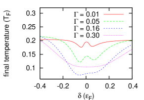
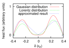
Note that for larger linewidths, the cooling works also for zero detuning $\delta$. Since $\delta$ plays the same role as voltage applied over an SN contact, this corresponds to cooling in presence of no external voltage. Such a system has been discussed recently in an interesting way in Pekola and Hekking (2007) where cooling by an SN junction is driven solely based on thermal noise from a resistor – the system is viewed as a Brownian refrigerator which conveys heat unidirectionally in response to external noise, in analogy to Brownian motors and thermal ratchets or to the concept of Maxwell’s demon. The effect of the thermal noise is to relax the energy conservation requirement in the tunneling process – in our case, this is done by the finite linewidth $\Gamma$ of the coupling field. We have derived an analytical estimate for the heat flux $\langle\dot{Q}_{N}\rangle$ defined in Eq.(3), using the following approximations: the Fermi distributions are approximated by their Boltzmann-like tails, the Lorentz distribution is replaced by a Gaussian of the same width, and the temperature and the linewidth are assumed to be smaller than the energy gap, also the detuning should be in the limits $|\delta|\lesssim\Delta$. The result becomes

$$\begin{split}&\frac{\dot{Q}_{N}}{N_{N}}=\frac{3\pi\hbar\Omega^{2}\sqrt{\mu}}{2\epsilon_{F}^{3/2}}e^{-\frac{\Delta}{T}}\bigg{\{}e^{\left(\frac{\Gamma^{2}}{2T^{2}}+\frac{|\delta|}{T}\right)}\times\\ &\left[\frac{\Gamma^{4}}{\Delta T^{2}}+2\Delta-3|\delta|+\frac{\delta^{2}}{\Delta}-\frac{3\Gamma^{2}}{T}+\frac{2\Gamma^{2}|\delta|}{\Delta T}+\frac{\Gamma^{2}}{\Delta}\right]\\ &-e^{-\frac{\Delta}{T_{S}}+\frac{\Delta}{T}}\left[2\Delta-3|\delta|+\frac{\delta^{2}}{\Delta}+\frac{\Gamma^{2}}{\Delta}\right]\bigg{\}}\end{split}$$ (4)

Here $T\equiv T_{N}$. The result can be compared to the one in Pekola and Hekking (2007) by substituting $\Gamma^{2}\rightarrow\sigma=2T_{R}E_{c}$ and $\delta\rightarrow E_{c}$. In Pekola and Hekking (2007) the variance $\sigma$ for the voltage arises from the temperature of the environment $T_{R}$, and contains the charging energy $E_{c}$ due to the junction and other capacitances. All the exponential factors are the same in our result and Pekola and Hekking (2007), however, the other terms differ, originating from the momentum conservation in our case. The analytical estimate (4) is compared to numerical results in Fig.3 by plotting the numerically calculated heat fluxes for a Gaussian and a Lorentz distribution, and the approximated result (4) for a Gaussian distribution. Fig.3 shows that the analytical estimate is reasonably good around the optimal detuning for cooling, however, one should use it with care for $\delta\simeq 0$. From Eq.(4) one can also estimate the optimal value for the linewidth, in two ways: one can either require a) the argument of the exponential to be zero, or b) those terms in the prefactor that are negative to be minimized. This gives $\Gamma=\sqrt{xT(\Delta+\delta)}$ where $x=2$ for case a) and $x=1$ for case b). Notably, this is the same condition as obtained in Pekola and Hekking (2007) for the optimal amount of “energy uncertainty” (variance $\sigma\propto T_{R}$) in the cooling process. For the parameters of Fig.2 the optimal linewidth given by these estimates is between $0.2\epsilon_{F}$ (a) and $0.14\epsilon_{F}$ (b) which is in excellent agreement with the numerically found optimal value $0.16\pm 0.01\epsilon_{F}$.

Figure 3: (Color online) Energy relative to chemical potential transferred out of the normal state (heat flux), $\langle\dot{Q}_{N}\rangle$, as a function of the detuning $\delta$. The curves are numerical results for Gaussian and Lorentz distributions, and approximate analytical result for a Gaussian distribution. The gap $\Delta=0.4\epsilon_{F}$, $T=0.1T_{F}$ and the linewidth $\Gamma=0.03\epsilon_{F}$.

Similarly, the heat flux out of the paired state becomes

$$\begin{split}&\frac{\dot{Q}_{S}}{N_{N}}=\frac{3\pi\Omega^{2}\sqrt{\mu}}{2}\bigg{[}(2\Delta-|\delta|)\times\\ &\left(e^{-\frac{\Delta}{T_{S}}}-e^{-\frac{\Delta}{T_{N}}+\frac{|\delta|}{T_{N}}+\frac{\Gamma^{2}}{2T_{N}^{2}}}\right)+\frac{\Gamma^{2}}{T_{N}}e^{-\frac{\Delta}{T_{N}}+\frac{|\delta|}{T_{N}}+\frac{\Gamma^{2}}{2T_{N}^{2}}}\bigg{]},\end{split}$$ (5)

where one can approximate the last term to be zero when $\Gamma^{2}/T_{N}<<\Delta$. One can see from here that, for suitable values of $T_{N}<T_{S}$, it is possible to cool the paired state as well. However, if $T_{N}\geq T_{S}$ cooling of the paired state is not possible because the factor $\frac{|\delta|}{T_{N}}+\frac{\Gamma^{2}}{2T_{N}^{2}}$ is always positive. This is in contrast to the case of Pekola and Hekking (2007) where the superconductor can be cooled (and the normal metal heated) also for $T_{N}=T_{S}$ in the case that the external resistor connected to the SN junction has a temperature $T_{R}$ lower than $T_{N}$. This illuminates the difference between the external reservoir (resistor) and the electromagnetic field: although thermal fluctuations of the reservoir in Pekola and Hekking (2007) and the linewidth of the field in our case have the same role in relaxing the energy conservation in tunneling, the reservoir can also increase its entropy in the process (if $T_{R}<T_{N}$) whereas the electromagnetic field does not have a role in the trade of entropy. In our case the entropy decreased by cooling the normal state simply increases the entropy of the paired state, and vice versa. E.g. if normal state is cooled from 0.2 $T_{F}$ to 0.1 $T_{F}$ the paired state heats from 0.2 $T_{F}$ to 0.29 $T_{F}$. To continue the cooling efficiently, the hot quasiparticles produced by the cooling pulse could be selectively removed away from the paired state, to a state that is not confined in the trap/lattice.

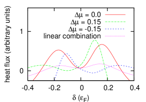
The proposed cooling method is not sensitive to having the chemical potentials equal, $\mu_{S}=\mu_{N}$, nor to homogeneity or completeness of the gap. This is demonstrated in Fig.4 where we show the heat flux for a non-balanced case $\mu_{N}\neq\mu_{S}$: cooling works even better, it only becomes asymmetric with respect to the detuning $\delta$. In practice, the paired state may well be different from the homogeneous space BCS-state used here, for instance the (pseudo)gap may be non-complete (i.e. it may have some spectral weight at zero energy as well), x-dependent, k-dependent, etc. In Fig.4 we show a linear combination of results for different gaps, simulating nodes and inhomogeneities in the gap in the spirit of local density approximation. The cooling is not dramatically affected, it is simply reduced in proportion with the inhomogeneity of the gap. The scheme also works for molecules but is not optimal because the pairing energy in that case easily becomes much larger than the temperature. In general, the cooling is based on coupling systems with different spectral densities which can be caused also by other effects than pairing, e.g. by Landau quantization Giazotto et al. (2007).

Figure 4: (Color online) The heat flux $\langle\dot{Q}_{N}\rangle$ out of the normal state. The curves are for various chemical potential differences $\Delta\mu=\mu_{S}-\mu_{N}$ between the paired and the normal state. The gap $\Delta=0.3\epsilon_{F}$, $T=0.1T_{F}$ and the linewidth $0.05\epsilon_{F}$. A linear combination of heat fluxes with different energy gaps, $\dot{Q}_{N}=0.1\dot{Q}_{N}(\Delta=0)+0.3\dot{Q}_{N}(\Delta=0.15)+0.6\dot{Q}_{N}(\Delta=0.3)$, is also shown.

The setting described here can be used for thermometry as well, as is also done in the solid state context Giazotto et al. (2006). The number of transferred particles becomes exponentially sensitive to temperature; calculating it in the same way as above gives the analytical estimate $\frac{\langle\Delta N_{N}\rangle}{N_{N}}\simeq\frac{3\pi^{2}\Omega\sqrt{\mu}}{2}\,\text{sgn}(\delta)\bigg{[}e^{-\frac{\Delta}{T_{N}}+\frac{|\delta|}{T_{N}}+\frac{\Gamma^{2}}{2T_{N}^{2}}}\times\left(2-\frac{|\delta|}{\Delta}-\frac{\Gamma^{2}}{\Delta T_{N}^{2}}\right)+e^{-\frac{\Delta}{T_{S}}}\left(2-\frac{|\delta|}{\Delta}\right)\bigg{]}.$

In summary, we have proposed cooling of a normal state Fermi gas, based on paired state – normal state tunneling created by electromagnetic fields. We have determined the optimal parameters for cooling and shown that temperature drops of the order of the pairing gap can be achieved. The cooling of a normal Fermi gas may find several applications. A promising one is to produce a very cold single-component Fermi gas, and subsequently turn on p-wave interactions by Feshbach resonance techniques. Especially in optical lattices, studies of p-wave pairing are of great interest due to the richness of the phase diagram. Our work also opens up a new connection and an opportunity for synergy between ultracold gases and solid state nanostructures research. In general, cooling-techniques are related to manipulation of the quasiparticle distributions of a quantum system, which is essential in the study of non-equilibrium effects.

Acknowledgements We thank T. Esslinger for useful discussions. This work was supported in part by the National Graduate School in Materials Physics, QUDEDIS, Academy of Finland (project numbers 106299, 213362, 115020) and National Science Foundation under Grant No. PHY05-51164, and conducted as part of a EURYI scheme award. See www.esf.org/euryi. J.K. acknowledges the support of the Department of Energy, Office of Basic Energy Sciences via the Chemical Sciences, Geosciences, and Biosciences Division.

References

- Anderson et al. (1995) M. H. Anderson et al., Science 269, 198 (1995).
- Davis et al. (1995) K. B. Davis et al., Phys. Rev. Lett. 75, 3969 (1995).
- Greiner et al. (2002) M. Greiner et al., Nature 415, 39 (2002).
- Jochim et al. (2003) S. Jochim et al., Science 302, 2101 (2003).
- Regal et al. (2003) C. Regal et al., Nature 426, 537 (2003).
- Regal et al. (2004) C. Regal et al., Phys. Rev. Lett. 92, 040403 (2004).
- Zwierlein et al. (2004) M. W. Zwierlein et al., Phys. Rev. Lett. 92, 120403 (2004).
- Bartenstein et al. (2004) M. Bartenstein et al., Phys. Rev. Lett. 92, 120401 (2004).
- Kinast et al. (2004) J. Kinast et al., Phys. Rev. Lett. 92, 150402 (2004).
- Chin et al. (2004) C. Chin et al., Science 305, 1128 (2004).
- Zwierlein et al. (2005) M. W. Zwierlein et al., Nature 435, 1047 (2005).
- Kinnunen et al. (2004) J. Kinnunen et al., Science 305, 1131 (2004).
- Giazotto et al. (2006) F. Giazotto et al., Rev. Mod. Phys. 78, 217 (2006).
- Mahan (2000) G. D. Mahan, Many-Particle Physics (Kluwer Academic/Plenum Publishers, New York, 2000).
- Törmä and Zoller (2000) P. Törmä and P. Zoller, Phys. Rev. Lett. 85, 487 (2000).
- Bruun et al. (2001) G. M. Bruun et al., Phys. Rev. A 64, 033609 (2001).
- Pekola and Hekking (2007) J. P. Pekola and F. W. J. Hekking (2007), eprint cond-mat/0702233.
- Giazotto et al. (2007) F. Giazotto et al. (2007), eprint cond-mat/0703119.