Langevin dynamics of the pure $SU(2)$ deconfining transition

Abstract

We investigate the dissipative real-time evolution of the order parameter for the deconfining transition in the pure $SU(2)$ gauge theory. The approach to equilibrium after a quench to temperatures well above the critical one is described by a Langevin equation. To fix completely the markovian Langevin dynamics we choose the dissipation coefficient, that is a function of the temperature, guided by preliminary Monte Carlo simulations for various temperatures. Assuming a relationship between Monte Carlo time and real time, we estimate the delay in thermalization brought about by dissipation and noise.

I Introduction

The study of the dynamics of phase conversion during the deconfinement transition for pure gauge theories might shed some light into the process of thermalization of the quark-gluon plasma in hot QCD in a controlled fashion. Indeed, for pure $SU(N)$, that can be seen as QCD in the limit of infinitely heavy quarks, lattice simulations are well developed, yielding a precise prediction for the deconfinement critical temperature and a good understanding of the corresponding thermodynamics Laermann:2003cv . In this limit there is a global $Z(N)$ symmetry associated with the center of the gauge group, so that one can use the Polyakov loop to construct a well-defined exact order parameter Polyakov:1978vu ; thooft , and an effective Landau-Ginzburg field theory based on this quantity pisarski ; ogilvie .

The effective potential for $T<<T_{d}$, where $T_{d}$ is the deconfinement critical temperature, has only one minimum, at the origin, where the whole system is localized. With the increase of the temperature, $N$ new minima appear. At the critical temperature, $T_{d}$, all the minima are degenerate, and above $T_{d}$ the new minima become the true vacuum states of the theory, so that the extremum at zero becomes unstable or metastable and the system starts to decay. In the case of $SU(3)$, whithin a range of temperatures close to $T_{d}$ there is a small barrier due to the weak first-order nature of the transition Bacilieri:1988yq , and the process of phase conversion will thus be guided by bubble nucleation. For larger $T$, the barrier disappears and the system explodes in the process of spinodal decomposition reviews . For $SU(2)$, the transition is second-order Damgaard:1987wh , and there is never a barrier to overcome.

Real-time relaxation to equilibrium after a thermal quench followed by a phase transition, as considered above, can in general be described by standard reaction-diffusion equations reviews . For a non-conserved order parameter, $\psi({\bf x},t)$, such as in the case of the deconfining transition in pure gauge theories, the evolution is given by the Langevin, or time-dependent Landau-Ginzburg, equation

$$\Gamma\,\frac{\partial\psi}{\partial t}=-\frac{\delta F}{\delta\psi}+\xi=-\sigma\left[\frac{\partial^{2}\psi}{\partial t^{2}}-\nabla^{2}\psi\right]-\frac{\partial U}{\partial\psi}+\xi\;,$$ (1)

where $F=F(\psi,T)$ is the coarse-grained free energy of the system, $\sigma$ is the surface tension and $U=U(\psi,T)$ is the effective potential. The quantity $\Gamma$ is known as the dissipation coefficient and will play an important role in our discussion. Its inverse defines a time scale for the system, and is usually taken to be either constant or as a function of temperature only, $\Gamma=\Gamma(T)$. The function $\xi$ is a stochastic noise assumed to be gaussian and white, so that

$$\langle\xi({\bf x},t)\rangle = 0\,,$$

$$\langle\xi({\bf x},t)\xi({\bf x}^{\prime},t^{\prime})\rangle = 2\Gamma\delta({\bf x}-{\bf x}^{\prime})\delta(t-t^{\prime})\,,$$ (2)

according to the fluctuation-dissipation theorem. From a microscopic point of view, the noise and dissipation terms are originated from thermal and quantum fluctuations resulting either from self-interactions of the field representing the order parameter or from the coupling of the order parameter to different fields in the system. In general, though, Langevin equations derived from a microscopic field theory micro contain also the influence of multiplicative noise and memory kernels FKR ; Koide:2006vf ; FKKMP .

In this paper, we consider the pure $SU(2)$ gauge theory, without dynamical quarks, that is rapidly driven to very high temperatures, well above $T_{d}$, and decays to the deconfined phase via spinodal decomposition. We are particularly interested in the effect of noise and dissipation on the time scales involved in this “decay process”, since this might provide some insight into the problem of thermalization of the quark-gluon plasma presumably formed in high-energy heavy ion collisions bnl . For the order parameter and effective potential we adopt the effective model proposed in Ref. ogilvie , and the choice of the dissipation coefficient, that is a function of the temperature, is guided by preliminary Monte Carlo simulations for various temperatures, comparing the short-time exponential growth of the two-point Polyakov loop correlation function predicted by the simulations Krein:2005wh to the Langevin description assuming, of course, that both dynamics are the same (see, also, the extensive studies of Glauber evolution by Berg et al. berg ). This procedure fixes completely the Markovian Langevin dynamics, as will be described below, if one assumes a relationship between Monte Carlo time and real time. Once the setup is defined for the real-time evolution, we can estimate the delay in thermalization brought about by dissipation and noise by performing numerical calculations for the dynamics of the order parameter on a cubic lattice. As will be shown in the following, the effects of dissipation and noise significantly delay the thermalization process for any physical choice of the parameters, a result that is in line with but is even more remarkable than the one found for the chiral transition Fraga:2004hp .

The paper is organized as follows. In Section II, we describe the effective model adopted for the Langevin evolution implementation, as well as the analytic behavior for early times. In Section III, we discuss the necessity of performing a lattice renormalization to have results that thermalize to values that are independent of the lattice spacing and free from ultraviolet divergences, and present the necessary counterterms. In Section IV we briefly describe the Glauber dynamics of pure lattice gauge theory that can be used to extract the dissipation coefficient for different values of the temperature. Details and quantitative results from lattice simulations will be presented in a future publication next . In Section V we present and analyze our numerical results for the time evolution of the order parameter for deconfinement after a quench to temperatures above $T_{d}$. Finally, Section VI contains our conclusions and outlook.

II Effective model and Langevin dynamics

Since we focus our investigation on pure gauge $SU(N)$ theories, we can adopt effective models built by using functions of the Polyakov loop as the order parameter for the deconfining phase transition. If quarks were included in the theory, the $Z(N)$ symmetry present in pure glue systems would be explicitly broken, and the Polyakov loop would provide only an approximate order parameter. For euclidean gauge theories at finite temperature, one defines the Polyakov loop as:

$$P(\vec{x})=\mathcal{T}\exp\left[ig\int^{1/T}_{0}d\tau A_{0}(\vec{x},\tau)\right]\,,$$ (3)

where $\mathcal{T}$ stands for euclidean time ordering, $g$ is the gauge coupling constant and $A_{0}$ is the time component of the vector potential.

The effective theory we adopt ogilvie is based on a mean-field treatment in which the Polyakov loops are constant throughout the space. The degrees of freedom that will be used to construct the free energy are the eigenvalues of the Polyakov loop, rather than $\langle Tr_{F}P(\vec{x})\rangle$. Working in $SU(N)$ gauge theories the Polyakov loop is unitary, so that it can be diagonalized by a unitary transformation, assuming the form

$$P_{jk}=\exp(i\theta_{j})\;\delta_{jk}\,.$$ (4)

At one loop, the free energy for gluons in a constant $A_{0}$ background is given by

$$f_{pert}(\theta)=ln[det(-D^{2}_{adj})]\,,$$ (5)

where $D_{adj}$ is the covariant derivative acting on fields in the adjoint representation. This expression can be written in a more explicit form:

$$f = -\frac{1}{\beta}\sum^{N}_{j,k=1}2\left(1-\frac{1}{N}\delta_{jk}\right)\times$$ (6)

$$\int\frac{d^{3}k}{(2\pi)^{3}}\sum_{n=1}^{\infty}\frac{1}{n}e^{-n\beta\omega_{k}+in\Delta\theta_{jk}}\,,$$

where $\theta$ is defined in Eq.(4), and $\Delta\theta_{jk}\equiv\theta_{j}-\theta_{k}$. Here we have the “bare” dispersion relation $\omega_{\bf k}\equiv|\bf k|$. In order to include confinement in this effective model description, one can introduce an ad hoc “thermal mass” for the gluons, so that the dispersion relation becomes $\omega_{\bf k}=\sqrt{{\bf k}^{2}+M^{2}}$. The value of $M$ can be related to the critical temperature $T_{d}$ extracted from lattice simulations.

Parametrizing the diagonalized Polyakov loop as $diag[\exp(i\phi_{N/2},...,i\phi_{1},-i\phi_{1},...,-i\phi_{N/2}]$, we can construct the effective potential from the free energy above. For $SU(2)$, it can be written in the following convenient form:

$$\frac{U}{T^{3}} = \frac{\pi^{2}}{60}-\frac{\pi^{2}}{6}\left(1-\frac{T_{d}^{2}}{T^{2}}\right)\psi^{2}+\frac{\pi^{2}}{12}\psi^{4}\;,$$ (7)

where we have defined $\psi\equiv 1-2\phi/\pi$, and used the relation between the mass $M$ and the critical temperature $T_{d}=\sqrt{3M^{2}/2\pi^{2}}$. In Fig. 1 we display $U$ as a function of $\psi$ for different values of the temperature. One can see from this plot that for $T\ll T_{d}$ the minimum is at $\psi({\bf x},t)=0$. As the temperature increases new minima appear; above the critical temperature they become the true vacuum states of the system. Now, if at $t=0$ the temperature is rapidly increased to $T\gg T_{d}$, the system is brought to an unstable state and therefore will start “rolling down” to the new minima of the effective potential.

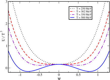
Figure 1: Effective potential for the case of $SU(2)$ for different values of the temperature.

To study the time evolution, we consider a system characterized by a coarse-grained free energy of the form

$$F(\psi,T)=\int d^{3}x\left[\frac{\sigma}{2}(\nabla\psi)^{2}+U(\psi,T)\right]\,,$$ (8)

where $U$ is the effective potential obtained above, and $\sigma$ plays the role of a surface tension Bhattacharya:1990hk , assuming the following value for $SU(2)$: $\sigma=\pi^{2}T/g^{2}$, $g$ being the gauge coupling. The approach to equilibrium of the order parameter $\psi({\bf x},t)$ will then be dictated by the Langevin equation (1) that, for arbitrary times, has to be solved numerically on a lattice.

At very short times, however, when $\psi(\mathbf{x},t)\approx 0$, non-linear terms in the evolution equation can be neglected, so that Eq. (1) reduces to

$$\sigma\ddot{\psi}_{\bf k}+\Gamma\dot{\psi}_{\bf k}+\sigma{\bf k}^{2}\psi_{\bf k}-T^{3}m_{T}^{2}\psi_{\bf k}\approx 0$$ (9)

in the Fourier space, where $m_{T}$ is a dimensionless thermal mass that can be written as

$$m_{T}^{2}=\frac{\pi^{2}}{3}\epsilon(T)=\frac{\pi^{2}}{3}\left(1-b~{}\frac{T_{d}^{2}}{T^{2}}\right)\,.$$ (10)

$b$ is a number that depends on the details of the quadratic term of the particular effective potential adopted, so that it will be different, for instance, if we consider $SU(2)$ ($b=1$) or $SU(3)$ ($b=10/9$). One can, then, approximate the (noiseless) solution in Fourier space by $\psi({\bf k},t\approx 0)\sim e^{\lambda_{\bf k}t}$, where $\lambda_{\bf k}$ are the roots of the quadratic equation

$$\lambda_{\bf k}^{2}+\left(\frac{\Gamma}{\sigma}\right)\lambda_{\bf k}+\left({\bf k}^{2}-\frac{T^{3}m_{T}^{2}}{\sigma}\right)=0\,.$$ (11)

For wavelength modes such that

$$|{\bf k}|<\left[\left(\frac{\Gamma}{2\sigma}\right)^{2}+\left(\frac{T^{3}m_{T}^{2}}{\sigma}\right)\right]^{1/2}\,,$$ (12)

one has already oscillations, but those are still damped by a factor $\exp(-\Gamma t/2\sigma)$. It is only for longer wavelength modes, i.e.

$$|{\bf k}|<k_{c}=\left(\frac{T^{3}m_{T}^{2}}{\sigma}\right)^{1/2}\,,$$ (13)

that there will be an explosive exponential growth corresponding to the regime of spinodal decomposition.

As time increases, the order parameter increases and non-linear contributions take over. To study the complete evolution of the phase conversion process, we have to solve $(\ref{TDLG})$ numerically on a lattice. In the next section we discuss the need for lattice renormalization to avoid spurious ultraviolet divergences in the dynamics.

III Lattice renormalization

In performing lattice simulations of the Langevin evolution, one should be careful in preserving the lattice-size independence of the results, especially when one is concerned about the behavior of the system in the continuum limit. In fact, in the presence of thermal noise, short and long wavelength modes are mixed during the dynamics, yielding an unphysical lattice size sensitivity. The issue of obtaining robust results, as well as the correct ultraviolet behavior, in performing Langevin dynamics was discussed by several authors Borrill:1996uq ; Bettencourt:1999kk ; Gagne:1999nh ; Bettencourt:2000bp ; krishna . The problem, which is not a priori evident in the Langevin formulation, is related to the well-known Rayleigh-Jeans ultraviolet catastrophe in classical field theory. The dynamics dictated by Eq. (1) is classical, and is ill-defined for very large momenta.

Equilibrium solutions of the Langevin equation that are insensitive to lattice spacing can be obtained, in practice, by adding finite-temperature counterterms to the original effective potential, which guarantees the correct short-wavelength behavior of the discrete theory. Furthermore, it assures that the system will evolve to the correct quantum state at large times. For a more detailed analysis of lattice renormalization in the Langevin evolution, including the case of multiplicative noise, see Ref. noise-broken .

Since the classical scalar theory in three spatial dimensions is super-renormalizable, only two Feynman diagrams are divergent, the tadpole and sunset. The singular part of these graphs can be isolated using lattice regularization, and then subtracted from the effective potential in the Langevin equation. For a scalar field theory, explicit expressions for the counterterms were obtained by Farakos et al. Farakos:1994kx within the framework of dimensional reduction in a different context.

Following Ref. Farakos:1994kx , we write the bare potential in a three-dimensional field theory in the following form

$${\cal V}(\phi)=-\frac{1}{2}m^{2}\phi^{2}+\frac{1}{4}\lambda_{3}\phi^{4}\,,$$ (14)

where $m$ is the bare mass of the field $\phi$ and the subindex in $\lambda_{3}$ stresses the fact that this is the coupling of a three-dimensional theory. In Ref. Farakos:1994kx , this dimensionally-reduced theory was obtained from a four-dimensional theory with a dimensionless coupling $\lambda$, assuming a regime of very high temperature. At leading order, one has $\lambda_{3}=\lambda\,T$. The mass counterterm, which is defined such that

$$-\frac{1}{2}\,m^{2}\,\phi^{2}\rightarrow-\frac{1}{2}\,\left(m^{2}+\delta m^{2}\right)\,\phi^{2}\equiv-\frac{1}{2}\,m^{2}_{R}\,\phi^{2}$$ (15)

is given by

$$\delta m^{2}=3\,\lambda_{3}\;\frac{0.252731}{a}-6\,\lambda^{2}_{3}\;\frac{1}{16\pi^{2}}\left[\ln\left(\frac{6}{\mu a}\right)+0.09\right]\,,$$ (16)

where $a$ is the lattice spacing and $\mu$ is the renormalization scale. The first term comes from the tadpode diagram and the second one from the sunset. Finite constants are obtained imposing that, after renormalization, the sunset diagram yields the same value for three renormalization schemes: lattice, momentum subtraction and $\overline{MS}$ Farakos:1994kx . Notice that in order to obtain lattice-independent results physical quantities become $\mu$-dependent Gagne:1999nh . However, since the contribution from the $\mu$-dependent term is logarithmic, variations around a given choice for this scale affect the final results by a numerically negligible factor, as we verified in our simulations, so that this dependence is very mild.

Since the field $\psi$ in the effective model we consider here is dimensionsless, it is convenient to define the dimensionful field $\varphi=\sigma^{1/2}\psi$ in order to relate results from Ref. Farakos:1994kx to our case more directly.

Now we can write our Langevin equation, Eq. (1), in terms of the field $\varphi$. For $SU(2)$, we have

$$\left(\frac{\partial^{2}\varphi}{\partial t^{2}}-\nabla^{2}\varphi\right)+\frac{\Gamma}{\sigma}\frac{\partial\varphi}{\partial t}-m^{2}_{L}\,\varphi+\lambda_{L}\varphi^{3}=\frac{\xi}{\sigma^{1/2}}\,$$ (17)

where

$$m^{2}_{L} = \frac{T^{3}m_{T}^{2}}{\sigma}=\frac{\epsilon(T)}{3}\,g^{2}\,T^{2}\,,$$ (18)

$$\lambda_{L} = \frac{\pi^{2}T^{3}}{3\sigma^{2}}=\frac{1}{3\pi^{2}}\,g^{4}\,T\,.$$ (19)

The subindex $L$ in these quantities is a reminder that they refer to the Langevin equation. It is clear that Eq. (17) corresponds to an effective action ${\cal S}(\varphi)$ given by

$${\cal S}(\varphi)=\frac{1}{2}(\nabla\varphi)^{2}-\frac{1}{2}m^{2}_{L}\,\varphi^{2}+\frac{1}{4}\lambda_{L}\,\varphi^{4}\,.$$ (20)

Once we have identified the mass term and the coupling constant, we can renormalize the Langevin equation, which becomes

$$\left(\frac{\partial^{2}\varphi}{\partial t^{2}}-\nabla^{2}\varphi\right)+\frac{\Gamma}{\sigma}\frac{\partial\varphi}{\partial t} = (m^{2}_{L}+\delta m^{2}_{L})\,\varphi$$ (21)

$$- \lambda_{L}\varphi^{3}+\frac{\xi}{\sigma^{1/2}}\,,$$

where

$$\delta m^{2}_{L}=3\,\lambda_{L}\;\frac{0.252731}{a}-6\,\lambda^{2}_{L}\;\frac{1}{16\pi^{2}}\left[\ln\left(\frac{6}{\mu a}\right)+0.09\right]\,..$$ (22)

Notice that we have used the same symbol $\varphi$ to denote both the renormalized and non-renormalized fields, since the theory is super-renormalizable and only mass counterterms are needed. In terms of the original $\psi$, our renormalized Langevin equation is finally given by

$$\frac{\pi^{2}T}{g^{2}}\left(\frac{\partial^{2}\psi}{\partial t^{2}}-\nabla^{2}\psi\right)+\Gamma\frac{\partial\psi}{\partial t} = \left[\frac{\pi^{2}T^{3}}{3}\epsilon(T)+\delta{\cal M}^{2}_{\psi}\right]\psi$$ (23)

$$- \frac{\pi^{2}T^{3}}{3}\psi^{3}+\zeta\,,$$

where

$$\delta{\cal M}^{2}_{\psi}=\frac{\pi^{2}T}{g^{2}}\;\delta m^{2}_{L}\,.$$ (24)

One can factor out the appropriate powers of $T$ in this expression to make explicit the mass dimensions:

$$\delta{\cal M}^{2}_{\psi} = 3\,T^{2}\,\frac{0.252731}{a}\left(\frac{g^{2}}{3}\right)$$

$$- 6\,T^{3}\,\frac{1}{16\pi^{2}}\left[\ln\left(\frac{6}{\mu a}\right)+0.09\right]\left(\frac{g^{2}}{3}\right)^{2}\left(\frac{g^{2}}{\pi}\right).$$

Notice that for sufficiently high temperatures the symmetry of the potential is restored.

IV Dissipation coefficient from Monte Carlo evolution

In lattice simulations for pure $SU(N)$ gauge theories, one can implement the Glauber dynamics by starting from thermalized gauge field configurations at a temperature $T<T_{d}$ and then changing the temperature of the entire lattice that is quenched to $T>T_{d}$ berg ; next . The gauge fields are then updated using the heat-bath algorithm of Ref. updating without over-relaxation. A “time” unit in this evolution is defined as one update of the entire lattice by visiting systematically one site at a time.

The structure function, defined as

$$S(k,\tau)=\langle\widetilde{L}_{F}(k,\tau)\widetilde{L}_{F}(-k,\tau)\rangle\,,$$ (26)

where $\widetilde{L}_{F}(k,\tau)$ is the Fourier transform of $L_{F}(x,\tau)$, the Polyakov loop in the fundamental representation, can be used to obtain the values of the dissipation coefficient, $\Gamma$, for different values of the final temperature, $T$, as follows. At early times, immediately after the quench, $\psi\simeq 0$ and one can neglect the terms proportional to $\psi^{3}$ and $\psi^{4}$ in the effective potential to first approximation. It is not difficult to show that at early times, when $\psi$ is small, the structure function can be written as

$$S(k,\tau)=S(k,0)\,\exp\left[2\omega(k)\,\tau\right]\,,$$ (27)

where

$$\omega(k)=\frac{\pi^{2}T}{g^{2}\Gamma}\;\left(k^{2}_{c}-k^{2}\right)\,.$$ (28)

In obtaining this expression we have neglected the second-order time derivative in Eq. (9), which should be a good approximation for a rough estimate of $\Gamma$. For the effective potential adopted here, $k^{2}_{c}$ is given by

$$k^{2}_{c}=\frac{g^{2}}{3}\left(T^{2}-\frac{9M^{2}}{4\pi^{2}}\right).$$ (29)

One sees that for momenta smaller than the critical momentum $k_{c}$, one has the familiar exponential growth, signaling spinodal decomposition. Plotting $\ln S(k,\tau)/\tau$ for different values of $k$ allows one to extract $2\omega(k)$ and, in particular, the value of $k^{2}_{c}$. Once one has extracted these values, $\Gamma$ can be obtained from the following relation:

$$\Gamma^{-1}=\omega(k)\,\frac{g^{2}}{\pi^{2}T(k^{2}-k^{2}_{c})}\,.$$ (30)

Now, in Monte Carlo simulations one does not have a time variable in physical units and so, by plotting $\ln S$ from the lattice, one obtains values of $2\omega(k)$ that do not include the (unknown) scale connecting real time $\tau$ and Monte Carlo time. Nevertheless, if one assumes that the relation between the Langevin time variable $\tau$ and the Monte Carlo time is linear, one can parametrize this relation in terms of the lattice spacing $a$ as $\tau=a\lambda_{MC}$, where $\lambda_{MC}$ is a dimensionless parameter that gives this relation in units of the lattice spacing. An estimate for the relationship between Monte Carlo time and real time is given in Ref. Tomboulis:2005es , where the authors evaluate the number of sweeps necessary for the system to freeze-out. In this reference, the authors implement lattice Monte Carlo simulations of the change of the Polyakov loop under lattice expansion and temperature falloff. The freeze-out number of sweeps was defined as being the number of sweeps necessary for the Polyakov loop to reach zero. This number was found to be of the order of $5000$ for the range of temperatures we are considering here. Using the phenomenological value of $9$ fm/c Kolb:2003gq as the freeze-out time, one can then obtain $\lambda_{MC}$.

Preliminary simulations clearly show that $\Gamma^{-1}$ decreases as the final temperature increases next . Guided by these results, we choose in the case of $SU(2)$ $\Gamma(T)=10^{3}~{}$fm^-2 for our Langevin simulations, which we describe in the next section.

V Numerical results for deconfinement and discussion

We solve Eq. (1) numericaly for $SU(2)$ in a cubic spacelike lattice with $64^{3}$ sites under periodic boundary conditions, using the semi-implicit finite-difference method for time discretization and finite-difference Fast Fourier Transform for spatial discretization and evolution copetti . To compute the expectation value of the order parameter $\psi$, we average over thousands of realizations with different initial conditions around $\psi\approx 0$ and different initial configurations for the noise. At each time step we compute

$$\langle\psi\rangle=\frac{1}{N^{3}}\sum_{ijk}\psi_{ijk}(t)\,,$$ (31)

where the indices $i,j,k$ indicate the position of the site on the lattice.

The thermal mass $M$ can be determined through the deconfinement temperature. For $SU(2)$, $T_{d}=302$ MeV, so that $M=775$ MeV. In Fig. 2 we show the time evolution of $\langle\psi\rangle$ for the $SU(2)$ case, normalized by $\psi_{0}$, which corresponds to the value of the order parameter at the vacuum. The dotted line represents the case with no noise and no dissipation, the dashed line corresponds to the case with only dissipation, and the full line to the complete case. Simulations were run under a temperature of $T=6.6\ T_{d}$, which ensures that there is no barrier to overcome, and the dynamics will be that of spinodal decomposition. For this temperature the value of $\Gamma$ is given by $10^{3}~{}$fm^-2, in accordance with the discussion of the previous section.

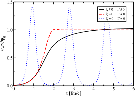
Figure 2: Langevin evolution of the $SU(2)$ order parameter.

One can clearly see from the figure that dissipation brings strong effects in the time evolution, delaying considerably the necessary time for the onset of the decay process. Noise acts in the same direction as dissipation, retarding even more the time of equilibration: from around $2$ fm/c, for the simulation including dissipation effects only, to more than $4$ fm/c in the complete case. Comparing our results to those from a similar calculation performed for the case of the chiral phase transition Fraga:2004hp , it is evident that in the former dissipation and noise have similar but stronger effects. This might signal that the dynamics of the deconfinement transition is more sensitive to medium effects. However, this is a very premature conjecture, since both effective theory approaches are rather simplified descriptions of in-medium QCD.

VI Conclusions and outlook

We have presented a systematic procedure to study the real-time dynamics of pure gauge deconfinement phase transitions, considering in detail the case of $SU(2)$. Given an effective field theory for the order parameter of the transition, we have discussed the necessity to introduce counterterms from lattice renormalization that guarantee lattice independence of physical results. These counterterms were computed for the case of $SU(2)$ or any theory whose effective model exhibits the same divergence structure.

For the Langevin evolution, one needs the dissipation coefficient as an input. We have described a recipe to extract this kinetic quantity from Glauber dynamics in Monte Carlo simulations. The value adopted here is based on preliminary lattice results. A detailed analysis will be presented in a future publication next , together with Langevin evolution results for the case of $SU(3)$.

From our results for the dynamics of the deconfining transition in $SU(2)$, we conclude that dissipation and noise play a very relevant role, being responsible for delays in the equilibration time of the order of $100\%$. So, effects from the medium are clearly significant in the determination of the physical time scales, and should be included in any description.

Of course, the treatment implemented here is very simplified in many respects. First, there is a need for a more robust effective theory for the order parameter of the deconfining transition. Recently, studies of the renormalization of Polyakov loops naturally lead to effective matrix models for the deconfinement transition matrix , unfolding a much richer set of possibilities than the approach considered here. In particular, eigenvalue repulsion from the Vandermonde determinant in the measure seems to play a key role as discussed in Ref. Pisarski:2006hz . Nevertheless, these studies have shown that, in the neighborhood of the transition, the relevant quantity is still the trace of the Polyakov loop.

Second, there is a need to construct a phenomenological generalized Landau-Ginzburg effective theory describing simultaneously the processes of chiral symmetry restoration and deconfinement in the presence of massive quarks as discussed in Ref. Fraga:2007un . Then, the dynamics of the approximate order parameters, the chiral condensate and the expectation value of the trace of the Polyakov loop, will be entangled. Finally, if one has the physics of heavy ion collisions in mind, effects brought about by the expansion of the plasma explosive and by its finite size Fraga:2003mu will also bring corrections to this picture.

In a more realistic approach, time scales extracted from the real-time evolution of the order parameters can be confronted with high-energy heavy ion collisions experimental data, and perhaps provide some clues for the understanding of the mechanism of equilibration of the quark-gluon plasma presumably formed at Relativistic Heavy Ion Collider (RHIC).

References

- (1) E. Laermann and O. Philipsen, Ann. Rev. Nucl. Part. Sci. 53, 163 (2003).
- (2) A. M. Polyakov, Phys. Lett. B 72, 477 (1978).
- (3) G. ’t Hooft, Nucl. Phys. B 138, 1 (1978); ibid. 153, 141 (1979).
- (4) R. D. Pisarski, Phys. Rev. D 62, 111501 (2000); A. Dumitru and R. D. Pisarski, Phys. Lett. B 504, 282 (2001); A. Dumitru, Y. Hatta, J. Lenaghan, K. Orginos and R. D. Pisarski, Phys. Rev. D 70, 034511 (2004); A. Dumitru, J. Lenaghan and R. D. Pisarski, Phys. Rev. D 71, 074004 (2005); A. Dumitru, R. D. Pisarski and D. Zschiesche, Phys. Rev. D 72, 065008 (2005).
- (5) T. R. Miller and M. C. Ogilvie, Phys. Lett. B 488, 313 (2000); P. N. Meisinger, T. R. Miller and M. C. Ogilvie, Phys. Rev. D 65, 034009 (2002).
- (6) P. Bacilieri et al., Phys. Rev. Lett. 61, 1545 (1988); F. R. Brown et al, Phys. Rev. Lett. 61 (1988) 2058.
- (7) J. D. Gunton, M. San Miguel and P. S. Sahni, in Phase Transitions and Critical Phenomena (Eds.: C. Domb and J. L. Lebowitz, Academic Press, London, 1983), vol. 8; N. Goldenfeld, Lectures on Phase Transitions and the Renormalization Group, (Addison-Wesley, New York, 1992); A. J. Bray, Adv. Phys. 43, 357 (1994).
- (8) P. H. Damgaard, Phys. Lett. B 194, 107 (1987); J. Engels et al, Phys. Lett. B 365, 219 (1996).
- (9) M. Gleiser and R. O. Ramos, Phys. Rev. D 50, 2441 (1994); C. Greiner and B. Muller, Phys. Rev. D 55, 1026 (1997); D. H. Rischke, Phys. Rev. C 58, 2331 (1998).
- (10) E. S. Fraga, G. Krein and R. O. Ramos, AIP Conf. Proc. 814, 621 (2006).
- (11) T. Koide, G. Krein and R. O. Ramos, Phys. Lett. B 636, 96 (2006).
- (12) E. S. Fraga, T. Kodama, G. Krein, A. J. Mizher and L. F. Palhares, Nucl. Phys. A 785, 138 (2007).
- (13) R. Stock, J. Phys. G 30, S633 (2004).
- (14) G. Krein, AIP Conf. Proc. 756, 419 (2005).
- (15) B. A. Berg et al., Nucl. Phys. Proc. Suppl. 129, 587 (2004); Phys. Rev. D 69, 034501 (2004); B. A. Berg, H. Meyer-Ortmanns and A. Velytsky, Phys. Rev. D 70, 054505 (2004); B. A. Berg, A. Velytsky and H. Meyer-Ortmanns, Nucl. Phys. Proc. Suppl. 140, 571 (2005); A. Bazavov, B. A. Berg and A. Velytsky, Nucl. Phys. Proc. Suppl. 140, 574 (2005); Int. J. Mod. Phys. A 20, 3459 (2005); hep-lat/0605001.
- (16) E. S. Fraga and G. Krein, Phys. Lett. B 614, 181 (2005).
- (17) G. Ananos, E. S. Fraga, G. Krein and A. J. Mizher, work in progress.
- (18) T. Bhattacharya, A. Gocksch, C. Korthals Altes and R. D. Pisarski, Phys. Rev. Lett. 66, 998 (1991); Nucl. Phys. B 383, 497 (1992).
- (19) J. Borrill and M. Gleiser, Nucl. Phys. B 483, 416 (1997).
- (20) L. M. A. Bettencourt, S. Habib and G. Lythe, Phys. Rev. D 60, 105039 (1999).
- (21) C. J. Gagne and M. Gleiser, Phys. Rev. E 61, 3483 (2000).
- (22) L. M. A. Bettencourt, Phys. Rev. D 63, 045020 (2001).
- (23) L. M. A. Bettencourt, K. Rajagopal and J. V. Steele, Nucl. Phys. A 693, 825 (2001).
- (24) N. C. Cassol-Seewald, R. L. S. Farias, E. S. Fraga, G. Krein and R. O. Ramos, to appear.
- (25) K. Farakos, K. Kajantie, K. Rummukainen and M. E. Shaposhnikov, Nucl. Phys. B 425, 67 (1994).
- (26) N. Cabibbo and E. Marinari, Phys. Lett. B 119, 387 (1982); A. D. Kennedy and B. J. Pendleton, Phys. Lett. B 156, 393 (1985).
- (27) E. T. Tomboulis and A. Velytsky, Phys. Rev. D 72, 074509 (2005).
- (28) P. F. Kolb, Heavy Ion Phys. 21, 243 (2004).
- (29) M.I.M. Copetti and C.M. Elliot, Mater. Sci. Tecnol. 6, 273 (1990).
- (30) A. Dumitru, Y. Hatta, J. Lenaghan, K. Orginos and R. D. Pisarski, Phys. Rev. D 70, 034511 (2004); A. Dumitru, J. Lenaghan and R. D. Pisarski, Phys. Rev. D 71, 074004 (2005); A. Dumitru, R. D. Pisarski and D. Zschiesche, Phys. Rev. D 72, 065008 (2005).
- (31) R. D. Pisarski, Phys. Rev. D 74, 121703 (2006); hep-ph/0612191.
- (32) E. Fraga and A. Mocsy, hep-ph/0701102.
- (33) A. Dumitru and R. D. Pisarski, Nucl. Phys. A 698, 444 (2002); O. Scavenius, A. Dumitru and A. D. Jackson, Phys. Rev. Lett. 87, 182302 (2001).
- (34) E. S. Fraga and R. Venugopalan, Physica A 345, 121 (2005).