hep-th/0704.3891
ITEP-TH-17/07
UUITP-07/07

1 Introduction

There has been much recent progress in the effort to completely establish the AdS/CFT correspondence [1, 2, 3]. The full conjectured integrability of planar $\mathcal{N}=4$ Super Yang-Mills [4, 5, 6] and its dual theory, the string sigma-model on an $\mathrm{AdS}_{5}\times S^{5}$ target space [7], has been instrumental in this progress. At least for the question of gauge operators of infinite bare dimension, computing the spectrum has basically come down to finding a two-particle S-matrix [8] that can be determined for both large and small values of the ’t Hooft coupling.

For large ’t Hooft coupling, the scattering is that of string oscillators on the world-sheet, while for small ’t Hooft coupling it more closely resembles the scattering of magnons on a spin-chain. Remarkably, as was shown by Beisert [9, 10], the S-matrix is almost completely determined by the underlying superalgebra $\mathfrak{su}(2|2)\times\mathfrak{su}(2|2)$ with central extension, no matter what the coupling. The only part of the S-matrix that cannot be determined from the supergroup structure itself is an overall phase factor (the dressing phase), which was conjectured first in the form of an asymptotic series at strong coupling [11], and then non-perturbatively [12]. First steps towards derivation of the dressing phase from Bethe ansatz were taken in the recent work [13, 14]. The conjectured dressing phase makes the S-matrix crossing-symmetric [15] and passes a remarkable four-loop test at weak ’t Hooft coupling: decoration of the Bethe equations with the conjectured phase modifies the anomalous dimensions starting from four loops and such a modification brings the Bethe-ansatz prediction for the cusp anomalous dimension [12] into agreement with the explicit four-loop calculation [16, 17].

It is remarkable that explicit four-loop calculations in $\mathcal{N}=4$ SYM are possible and it is certainly desirable to reach comparable accuracy on the string side. Currently, state of the art is the one-loop order: quantum corrections to the energies of various classical string configurations have been computed in [18, 19, 20]. The purpose of this paper is to go beyond the one-loop order. Since the full $\mathrm{AdS}_{5}\times S^{5}$ sigma-model [21] is quite complicated we make use of the simplifying limit proposed recently by Maldacena and Swanson [22].

As in [23, 24], we will be interested in the world-sheet S-matrix which can be directly compared to the $\mathfrak{su}(2|2)\times\mathfrak{su}(2|2)$ S-matrix [9, 10] with the conjectured dressing phase [11, 12]. The world-sheet S-matrix simplifies immensely in the Maldacena-Swanson limit, but is nonetheless nontrivial since the resulting sigma model is still interacting. The limit is taken by scaling all momenta, such that $p\lambda^{1/4}$ is finite. The momenta of the string excitations then sit in the “near-flat” region, between the noninteracting BMN regime [25] and the classical giant magnon regime of [26]. For excitations in the near-flat region, although there is no $\sin p/2$ factor in the dispersion relation like in the case for giant magnons, the Lorentz invariance of the BMN region is still broken by interaction terms. However, as we will show this breaking of Lorentz invariance is rather mild, and in fact can be restored if one compensates any Lorentz boost with a rescaling of the world-sheet coupling constant. It might be possible to argue that the S-matrix satisfies the usual crossing symmetry as a consequence of the usual LSZ theorems, with additional modifications due to this ”soft” breaking of Lorentz invariance. We shall see that the crossing symmetry is certainly there at the level of Feynman diagrams.

The near-flat limit also leads to a simplification of the Janik’s equation [15]. The odd solution will still be a sum of dilogarithms, but the even phase simplifies tremendously and will end up being the log of a rational function of the world-sheet coupling (and so its contribution to the S-matrix is to multiply it by a rational function). It is simple to check that this function is a solution to the near-flat limit of the BHL even equation. The S-matrix for the various processes also turns out to be a quadratic polynomial of the world-sheet coupling multiplied by a common function.

Computing quantum corrections is much simpler in the near-flat limit. The quartic nature of the interaction terms makes the computations similar to those found in $\phi^{4}$ theory in two dimensions. For two-point functions, supersymmetry prevents any tadpoles from occuring, so there is no one-loop wave function renormalization or mass-shift. However, at the two-loop level there are sunset diagrams which induce radiative corrections to the dispersion relation that agree with the predicted near-flat limit of the dispersion relation in [22].

We then consider corrections to the four point amplitudes. We will compute these corrections up to the two-loop level, where we will find agreement with the near-flat limit of the BHL prediction. This provides the first nontrivial check that goes beyond the tree level AFS [27] and one-loop HL [28] dressing factor terms. In carrying out these computations, we will see that the final amplitudes for the different processes are very similar, as they must be if they are to agree with the BHL S-matrix, but the road to how these final amplitudes are reached can be significantly different. For example, for certain $2\rightarrow 2$ bosonic processes, there is a four-fermion interaction term that contributes to the two-loop amplitude, while in other processes this interaction term plays no role. In any case, the underlying supersymmetry must play a crucial part in determining the final structure of these amplitudes. In going from the amplitude to the S-matrix, we must take into account the two-loop wave-function renormalization as well as the two-loop mass-shift which will affect the Jacobian factor that needs to be included.

This paper is structured as follows. In Sec. 2 we review Maldacena and Swanson’s action for the near-flat limit. In Sec. 3 we consider the two-loop two-point functions, where we explicitly compute the wave-function renormalization and mass-shift. In Sec. 4 we derive the near-flat limit of the conjectured S-matrix. In Sec. 5 we find the one-loop four-point amplitudes while in Sec. 6 we find these amplitudes at two loops. In these last two sections we also show that these results are in agreement with the results in Sec. 4. In Sec. 7 we present our conclusions. We also include several appendices which contain some of the technical details of our calculations.

2 Near-flat-space model

Our starting point is the relatively simple light-cone action for the reduced model of [22](in the notation of [24]):

$$\mathcal{L} = \frac{1}{2}(\partial Y)^{2}-\frac{m^{2}}{2}\,Y^{2}+\frac{1}{2}(\partial Z)^{2}-\frac{m^{2}}{2}\,Z^{2}+\frac{i}{2}\,\psi\,\frac{\partial^{2}+m^{2}}{\partial_{-}}\,\psi$$ (2.1)

$$+\gamma\,(Y^{2}-Z^{2})\bigl{(}(\partial_{-}Y)^{2}+(\partial_{-}Z)^{2}\bigr{)}+i\gamma\,(Y^{2}-Z^{2})\psi\partial_{-}\psi$$

$$+i\gamma\,\psi\bigl{(}\partial_{-}Y^{i^{\prime}}\mathnormal{\Gamma}^{i^{\prime}}+\partial_{-}Z^{i}\mathnormal{\Gamma}^{i}\bigr{)}\bigl{(}Y^{i^{\prime}}\mathnormal{\Gamma}^{i^{\prime}}-Z^{i}\mathnormal{\Gamma}^{i}\bigr{)}\psi$$

$$-\frac{\gamma}{24}\bigl{(}\psi\mathnormal{\Gamma}^{i^{\prime}j^{\prime}}\psi\,\psi\mathnormal{\Gamma}^{i^{\prime}j^{\prime}}\psi-\psi\mathnormal{\Gamma}^{ij}\psi\,\psi\mathnormal{\Gamma}^{ij}\psi\bigr{)}.$$

The bosonic fields $Z^{i}$ and $Y^{i^{\prime}}$ correspond to transverse excitations in the $AdS_{5}$ and $S^{5}$ directions respectively and the fermions, $\psi$, are Majorana-Weyl $\mathrm{SO}(8)$ spinors of positive chirality. The action in 2.1 is not invariant under world-sheet Lorentz transformations, but it is invariant under 8 independent linearly realized supersymmetries.

This action is the same as the near-flat space truncation of [22], however as in [24], we have introduced the parameter $\gamma$ by rescaling the worldsheet coordinates and furthermore we have integrated out the half of the original sixteen fermions which occured only quadratically in the action. The near-flat space action action of [22] was obtained from $\mathrm{AdS}_{5}\times S^{5}$ string sigma-model by expanding about a constant density solution boosted with rapidity $\sim\lambda^{1/4}$ in the $\sigma^{-}$ direction and so the above truncation should be equivalent to the full theory in the near-flat limit,

$$p_{-}\sim\sqrt[4]{\lambda}\quad,\quad p_{+}\sim\frac{1}{\sqrt[4]{\lambda}}\,$$ (2.2)

provided we set

$$\gamma=\frac{\pi}{\sqrt{\lambda}}$$ (2.3)

and the mass, $m$, to be unity.

3 Two-loop propagator

We now turn to the computation of the two-loop correction to the propagator. Firstly, we confirm that this leads to the expected mass shift and therefore the expected corrections to the dispersion relation. Secondly, for our two-loop scattering computation in Sec. 6, it is necessary to know the residue of the pole in the propagator, which we determine here as well.

The dispersion relation in the original sigma model is expected to be

$$\varepsilon=m\sqrt{1+\frac{1}{\gamma^{2}}\sin^{2}\frac{\gamma p}{m}}\xrightarrow{\;\;\;(\ref{eqn:MSlimit})\;\;}\sqrt{m^{2}+p^{2}-\frac{\gamma^{2}p_{-}^{4}}{3m^{2}}}\;.$$ (3.1)

The second expression is the predicted exact dispersion relation in the near-flat limit (2.2). We will now derive this dispersion relation from a Feynman diagram computation in the model (2.1). This computation shows for the first time the emergence of the sine in the dispersion relation from the perturbation expansion of the string sigma-model.

The first correction to the propagator is of order $\gamma^{2}$ and the corresponding diagram is the sunset diagram drawn in Fig. 3(b) on page 3(b). Doing the combinatorics for the bosonic and the fermionic propagator, respectively, leads to

$$\begin{split}\mathcal{A}_{b}(p)&=32i\gamma^{2}\left[2p_{-}^{2}\left(2I_{110}+I_{200}\right)-p_{-}\left(I_{111}+I_{210}\right)+\left(4I_{211}+I_{220}+I_{310}\right)\right]\\ \mathcal{A}_{f}(p)&=16i\gamma^{2}\left[p_{-}^{2}I_{100}+2p_{-}I_{200}+6I_{111}+14I_{210}+I_{300}\right]\end{split}$$ (3.2)

where

$$I_{rst}(p)=\int\frac{d^{2}\mathbf{k}\,d^{2}\mathbf{q}}{(2\pi)^{4}}\frac{(k_{-})^{r}\,(q_{-})^{s}\,(p_{-}-k_{-}-q_{-})^{t}}{(\mathbf{k}^{2}-m^{2})(\mathbf{q}^{2}-m^{2})[(\mathbf{p}-\mathbf{k}-\mathbf{q})^{2}-m^{2}]}\;.$$ (3.3)

This integral is the sunset diagram with $r$, $s$ and $t$ powers of the three momenta inserted into the numerator, cf. App. B.2. Some of these factors originate from derivative couplings, others are due to the extra power of $p_{-}$ in the fermionic propagator. We can simplify the expression for the amplitudes using the identity

$$p_{-}I_{rst}=I_{r+1,s,t}+I_{r,s+1,t}+I_{r,s,t+1}\;.$$ (3.4)

Applying this identity repeatedly, we find that the amplitudes simplify to

$$\mathcal{A}_{b}(p)=\frac{64}{3}i\gamma^{2}p_{-}^{4}I_{000}(\mathbf{p}^{2})\quad,\quad\mathcal{A}_{f}(p)=\frac{64}{3}i\gamma^{2}p_{-}^{3}I_{000}(\mathbf{p}^{2})\;,$$ (3.5)

where $I_{000}$ is a function of $\mathbf{p}^{2}$ only. It is interesting to see how the very different structures in (3.2) reduce to essentially the same expression. We perform this integral in App. B.2 and find for the on-shell amplitudes

$$\mathcal{A}_{b}(p)=i\gamma^{2}\frac{p_{-}^{4}}{3m^{2}}\quad,\quad\mathcal{A}_{f}(p)=i\gamma^{2}\frac{p_{-}^{3}}{3m^{2}}\;.$$ (3.6)

In order to find the corrected dispersion relation, we consider the iteration of sunset diagrams (3.5). Via a geometric series this leads to the corrected propagator

$$\frac{i}{\mathbf{p}^{2}-m^{2}+\frac{64}{3}i\gamma^{2}p_{-}^{4}I_{000}(\mathbf{p})}\stackrel{{\scriptstyle!}}{{=}}\frac{iZ(p_{-})}{2p_{+}-\mathnormal{\Sigma}(p_{-})}+\mbox{finite as $2p_{+}\to\mathnormal{\Sigma}(p_{-})$}\;,$$ (3.7)

where there is an extra factor of $p_{-}$ in the numerator for the fermionic propagator. The right hand side of (3.7) defines the position $\mathnormal{\Sigma}(p_{-})$ and the residue $Z(p_{-})$ of the pole in the propagator in the $2p_{+}$ plane. Note that for our definition of the light-cone momenta (C.1), $2p_{+}$ is the appropriate “energy” for time evolution in $\sigma^{+}$ direction.

The dispersion relation is determined by the pole in the propagator. To order $\gamma^{2}$ we only need the on-shell value (B.7) of the integral $I_{000}$ and find

$$p_{+}(p_{-})=\frac{1}{2}\mathnormal{\Sigma}(p_{-})=\frac{m^{2}}{4p_{-}}-\frac{\gamma^{2}p_{-}^{3}}{12m^{2}}\;.$$ (3.8)

Using $\varepsilon^{2}-p^{2}=4p_{+}p_{-}$, we convert this equation into the form $\varepsilon(p)$ and find that this dispersion relation exactly agrees with the prediction in (3.1).

For computing the residue we also need the on-shell value of the first derivative of $I_{000}$ with respect to $\mathbf{p}^{2}$. Taking this integral from (B.8), we find the wave-function renormalization to order $\gamma^{2}$ to be

$$Z(p_{-})=\frac{1}{2p_{-}}\left[1-\frac{\gamma^{2}}{m^{4}}\left(\frac{1}{\pi^{2}}-\frac{1}{12}\right)p_{-}^{4}\right]\;.$$ (3.9)

This correction is an important contribution to the two-loop amplitudes which we compute in Sec. 6. It will turn out that this correction cancels the entire wineglass contribution in the $t$-channel.

4 $\mathrm{SU}(2|2)$ S-matrix

The $\mathrm{SU}(2|2)$ scattering matrix is expressed in terms of the following kinematic variables:

$$x_{\pm}(p)=\frac{1+\sqrt{1+P^{2}}}{P}\,\,{\rm e}\,^{\pm\frac{i\pi p}{\sqrt{\lambda}}}\;,\qquad P=\frac{\sqrt{\lambda}}{\pi}\,\sin\frac{\pi p}{\sqrt{\lambda}}\;.$$ (4.1)

For the S-matrix components, we use the conventions of [23]:

$$\quad{S}_{{a}{b}}^{{c}{d}} ={A}\,\delta_{a}^{c}\delta_{b}^{d}+{B}\,\delta_{a}^{d}\delta_{b}^{c}\;, {S}_{{a}{b}}^{{\gamma}{\delta}} ={C}\,\epsilon_{{a}{b}}\epsilon^{{\gamma}{\delta}}\;,$$

$${S}_{{\alpha}{\beta}}^{{\gamma}{\delta}} ={D}\,\delta_{\alpha}^{\gamma}\delta_{\beta}^{\delta}+{E}\,\delta_{\alpha}^{\delta}\delta_{\beta}^{\gamma}\;, {S}_{{\alpha}{\beta}}^{{c}{d}} ={F}\,\epsilon_{{\alpha}{\beta}}\epsilon^{{c}{d}}\;,$$ (4.2)

$${S}_{{a}{\beta}}^{{c}{\delta}} ={G}\,\delta_{a}^{c}\delta_{\beta}^{\delta}\;, {S}_{{a}{\beta}}^{{\gamma}{d}} ={H}\,\delta_{a}^{d}\delta_{\beta}^{\gamma}\;,$$

$${S}_{{\alpha}{b}}^{{\gamma}{d}} ={L}\,\delta_{\alpha}^{\gamma}\delta_{b}^{d}\;, {S}_{{\alpha}{b}}^{{c}{\delta}} ={K}\,\delta_{\alpha}^{\delta}\delta_{b}^{c}\;.$$

The explicit expressions for matrix elements are [9]:

$${A}=\frac{x^{\prime}_{-}-x_{-}}{x^{\prime}_{-}-x_{+}}\,\,\frac{1-\frac{1}{x^{\prime}_{-}x_{+}}}{1-\frac{1}{x^{\prime}_{+}x_{+}}}\;,$$

$${B}=\frac{x^{\prime}_{+}-x_{-}}{x^{\prime}_{-}-x_{+}}\left(1-\frac{x^{\prime}_{-}-x_{-}}{x^{\prime}_{+}-x_{-}}\,\,\frac{1-\frac{1}{x^{\prime}_{-}x_{+}}}{1-\frac{1}{x^{\prime}_{+}x_{+}}}\right)\;,$$

$${C}=\frac{i\eta\eta^{\prime}}{x_{+}x^{\prime}_{+}}\,\,\frac{1}{1-\frac{1}{x^{\prime}_{+}x_{+}}}\,\,\frac{x^{\prime}_{-}-x_{-}}{x^{\prime}_{-}-x_{+}}\,\,{\rm e}\,^{\frac{i\pi p^{\prime}_{1}}{\sqrt{\lambda}}}\;,$$

$${D}=\frac{x^{\prime}_{+}-x_{+}}{x^{\prime}_{-}-x_{+}}\,\,\frac{1-\frac{1}{x^{\prime}_{+}x_{-}}}{1-\frac{1}{x^{\prime}_{-}x_{-}}}\,\,{\rm e}\,^{\frac{i\pi(p^{\prime}_{1}-p_{1})}{\sqrt{\lambda}}}\;,$$

$${E}=1-\frac{x^{\prime}_{+}-x_{+}}{x^{\prime}_{-}-x_{+}}\,\,\frac{1-\frac{1}{x^{\prime}_{+}x_{-}}}{1-\frac{1}{x^{\prime}_{-}x_{-}}}\,\,{\rm e}\,^{\frac{i\pi(p^{\prime}_{1}-p_{1})}{\sqrt{\lambda}}}\;,$$

$${F}=-\frac{i(x_{+}-x_{-})(x^{\prime}_{+}-x^{\prime}_{-})}{\eta\eta^{\prime}x_{-}x^{\prime}_{-}}\,\,\frac{1}{1-\frac{1}{x^{\prime}_{-}x_{-}}}\,\,\frac{x^{\prime}_{+}-x_{+}}{x^{\prime}_{-}-x_{+}}\,\,{\rm e}\,^{-\frac{i\pi p_{1}}{\sqrt{\lambda}}}\;,$$

$${G}=\frac{x^{\prime}_{+}-x_{+}}{x^{\prime}_{-}-x_{+}}\,\,{\rm e}\,^{-\frac{i\pi p_{1}}{\sqrt{\lambda}}}\;,\qquad\quad{H}=\frac{\eta}{\eta^{\prime}}\,\,\frac{x^{\prime}_{+}-x^{\prime}_{-}}{x^{\prime}_{-}-x_{+}}\,\,{\rm e}\,^{\frac{i\pi(p^{\prime}_{1}-p_{1})}{\sqrt{\lambda}}}\;,$$

$${L}=\frac{x^{\prime}_{-}-x_{-}}{x^{\prime}_{-}-x_{+}}\,\,{\rm e}\,^{\frac{i\pi p^{\prime}_{1}}{\sqrt{\lambda}}}\;,\qquad\qquad{K}=\frac{\eta^{\prime}}{\eta}\,\,\frac{x_{+}-x_{-}}{x^{\prime}_{-}-x_{+}}\;,$$ (4.3)

where $x_{\pm}\equiv x_{\pm}(p)$, $x^{\prime}_{\pm}\equiv x_{\pm}(p^{\prime})$ and

$$\eta={|x_{-}-x_{+}|}^{1/2},\qquad\eta^{\prime}={|x^{\prime}_{-}-x^{\prime}_{+}|}^{1/2}\;.$$ (4.4)

The sigma-model scattering matrix is the tensor product of the two $\mathrm{SU}(2|2)$ S-matrices. The world-sheet scattering amplitudes are thus quadratic in the $A,B,C,D,\ldots$. In addition the world-sheet scattering matrix contains an overall phase factor:

$$\mathbbm{S}=\frac{1-\frac{1}{x^{\prime}_{+}x_{-}}}{1-\frac{1}{x^{\prime}_{-}x_{+}}}\,\,\frac{x^{\prime}_{-}-x_{+}}{x^{\prime}_{+}-x_{-}}\,\,{\rm e}\,^{i\theta(p,p^{\prime})}\,\,{S}\otimes{S}\;,$$ (4.5)

where $\theta(p,p^{\prime})$ is the dressing phase. For reader’s convenience we have written the action of $\mathbbm{S}$ on all two-particle states in App. D in order to see which matrix elements govern which processes.

The dressing phase has the following general form [27, 30]:

$$\theta(p,p^{\prime})=\sum_{r,s=\pm}rs\,\chi(x_{r},x^{\prime}_{s})\;.$$ (4.6)

The function $\chi(x,y)$ is anti-symmetric in $x$ and $y$ and can be expanded in asymptotic power series in $\pi/\sqrt{\lambda}$. We only need the first three orders of this expansion:

$$\chi(x,y) = \frac{\sqrt{\lambda}}{2\pi}\left(x-y\right)\left(1-\frac{1}{xy}\right)\ln\left(1-\frac{1}{xy}\right)$$ (4.7)

$$+\int_{0}^{1}\frac{dt}{\pi t}\,\,\ln\left[\frac{(1-t)^{2}xy-(t-x)^{2}}{(1-t)^{2}xy-(t+x)^{2}}\,\,\frac{(1-t)^{2}xy-(t+y)^{2}}{(1-t)^{2}xy-(t-y)^{2}}\right]$$

$$+\frac{\pi}{3\sqrt{\lambda}}\,\,\frac{xy+1}{xy-1}\,\,\frac{x-y}{\left(x^{2}-1\right)\left(y^{2}-1\right)}+\ldots\;.$$

The first line is the AFS tree-level phase [27], the second line is the HL one-loop correction [28] and the third line is taken from [11]. The integral in the one-loop phase can be expressed in terms of the dilogarithms, but for our purposes the integral representation is more convenient. The first and last lines are part of BHL’s even phase, while the middle line makes up the entire odd phase.

In the near-flat limit, the kinematic variables $x_{\pm}$ approach $-1$. However, the S-matrix contains many expressions of the form $x_{r}x^{\prime}_{s}-1$ or $x_{r}-x^{\prime}_{s}$ which vanish at $x_{r}=-1=x^{\prime}_{s}$. Plugging in $-1$ for $x_{\pm}$, $x^{\prime}_{\pm}$ produces singularities and we need to keep the next term in the expansion:

$$x_{\pm}=-1-\frac{1}{p_{-}}\pm\frac{i\pi}{\sqrt{\lambda}}\,p_{-}+\ldots\;.$$ (4.8)

The second and the third terms are small compared to one (they are of order $\mathcal{O}(\lambda^{-1/4})$) and should be omitted wherever $-1$ does not cancel.

We thus get

$$\mathbbm{S}=\frac{1-\frac{i\pi}{\sqrt{\lambda}}\,p_{-}p^{\prime}_{-}\,\frac{p^{\prime}_{-}-p_{-}}{p^{\prime}_{-}+p_{-}}}{1+\frac{i\pi}{\sqrt{\lambda}}\,p_{-}p^{\prime}_{-}\,\frac{p^{\prime}_{-}-p_{-}}{p^{\prime}_{-}+p_{-}}}\,\,\frac{\,{\rm e}\,^{i\theta(p,p^{\prime})}}{1+\frac{\pi^{2}}{\lambda}\,p_{-}^{2}p^{\prime}{}^{2}_{-}\left(\frac{p^{\prime}_{-}+p_{-}}{p^{\prime}_{-}-p_{-}}\right)^{2}}\,{S}\otimes{S}$$ (4.9)

where the matrix elements are as in (4.2) with

$${A} =1+\frac{i\pi}{\sqrt{\lambda}}\,p_{-}p^{\prime}_{-}\,\frac{p^{\prime}_{-}-p_{-}}{p^{\prime}_{-}+p_{-}}\;, {B} =-{E}=\frac{4i\pi}{\sqrt{\lambda}}\,\,\frac{p_{-}^{2}p^{\prime}{}^{2}_{-}}{p_{-}^{\prime 2}-p_{-}^{2}}\;,$$

$${D} =1-\frac{i\pi}{\sqrt{\lambda}}\,p_{-}p^{\prime}_{-}\,\frac{p^{\prime}_{-}-p_{-}}{p^{\prime}_{-}+p_{-}}\;, {C} ={F}=\frac{2i\pi}{\sqrt{\lambda}}\,\,\frac{p_{-}^{3/2}p_{-}^{\prime 3/2}}{p_{-}^{\prime}+p_{-}}\;,$$

$${G} =1+\frac{i\pi}{\sqrt{\lambda}}\,p_{-}p^{\prime}_{-}\;, {H} ={K}=\frac{2i\pi}{\sqrt{\lambda}}\,\,\frac{p_{-}^{3/2}p_{-}^{\prime 3/2}}{p_{-}^{\prime}-p_{-}}\;,$$

$${L} =1-\frac{i\pi}{\sqrt{\lambda}}\,p_{-}p^{\prime}_{-}\;.$$ (4.10)

We should stress that these expressions are exact in the near-flat limit. For comparison to the two-loop calculation in Sec. 6 we need to further expand in $\pi p_{-}^{2}/\sqrt{\lambda}$.

When expanding the phase in $\pi/\sqrt{\lambda}$ it is important to remember that it implicitly depends on $\lambda$ through $x_{\pm}$, apart from the explicit dependence manifest in (4.7). In particular the tree-level term in (4.7) contains a two-loop correction to the phase. The substitution of (4.8) into (4.6), (4.7) yields after a lengthy but straightforward calculation:

$$\theta(p,p^{\prime}) = \frac{2\pi}{\sqrt{\lambda}}\,p_{-}p^{\prime}_{-}\,\frac{p^{\prime}_{-}-p_{-}}{p^{\prime}_{-}+p_{-}}-\frac{4\pi^{3}}{3\lambda^{3/2}}\,p_{-}^{3}p^{\prime}{}^{3}_{-}\,\frac{(p^{\prime}_{-}-p_{-})(p^{\prime}{}^{2}_{-}+p_{-}p^{\prime}_{-}+p^{2}_{-})}{(p^{\prime}_{-}+p_{-})^{3}}$$ (4.11)

$$+\frac{8\pi}{\lambda}\,\,\frac{p^{3}_{-}p^{\prime}{}^{3}_{-}}{p^{\prime}{}^{2}_{-}-p^{2}_{-}}\left(1-\frac{p^{\prime}{}^{2}_{-}+p_{-}^{2}}{p^{\prime}{}^{2}_{-}-p_{-}^{2}}\,\ln\frac{p^{\prime}_{-}}{p_{-}}\right)$$

$$+\frac{2\pi^{3}}{3\lambda^{3/2}}\,p^{3}_{-}p^{\prime}{}^{3}_{-}\,\frac{(p^{\prime}_{-}-p_{-})(p^{\prime}{}^{2}_{-}+4p_{-}p^{\prime}_{-}+p^{2}_{-})}{(p^{\prime}_{-}+p_{-})^{3}}+\ldots\,.$$

Omitting $\mathcal{O}\left(\bigl{(}\frac{p}{\sqrt[4]{\lambda}}\bigr{)}^{6}\right)$ terms this can be written in the following nice form, suggested by the main scattering term,

$$\theta(p,p^{\prime})=-i\ln\frac{1+\frac{i\pi}{\sqrt{\lambda}}\,p_{-}p^{\prime}_{-}\,\frac{p^{\prime}_{-}-p_{-}}{p^{\prime}_{-}+p_{-}}}{1-\frac{i\pi}{\sqrt{\lambda}}\,p_{-}p^{\prime}_{-}\,\frac{p^{\prime}_{-}-p_{-}}{p^{\prime}_{-}+p_{-}}}+\frac{8\pi}{\lambda}\,\,\frac{p^{3}_{-}p^{\prime}{}^{3}_{-}}{p^{\prime}{}^{2}_{-}-p^{2}_{-}}\left(1-\frac{p^{\prime}{}^{2}_{-}+p_{-}^{2}}{p^{\prime}{}^{2}_{-}-p_{-}^{2}}\,\ln\frac{p^{\prime}_{-}}{p_{-}}\right),$$ (4.12)

where the first (second) term comes from the even (odd) phase . Equation (4.9) becomes

$$\mathbbm{S}=S_{0}\,{S}\otimes{S}\quad\mbox{with}\quad S_{0}=\frac{\,\,e^{\frac{8\pi i}{\lambda}\,\,\frac{p^{3}_{-}p^{\prime}{}^{3}_{-}}{p^{\prime}{}^{2}_{-}-p^{2}_{-}}\left(1-\frac{p^{\prime}{}^{2}_{-}+p_{-}^{2}}{p^{\prime}{}^{2}_{-}-p_{-}^{2}}\,\ln\frac{p^{\prime}_{-}}{p_{-}}\right)}}{1+\frac{\pi^{2}}{\lambda}\,p_{-}^{2}p^{\prime}{}^{2}_{-}\left(\frac{p^{\prime}_{-}+p_{-}}{p^{\prime}_{-}-p_{-}}\right)^{2}}$$ (4.13)

where ${S}$ is given by (4.2), (4). At the end, the dressing phase almost completely cancels the main scattering phase, and the two-loop prediction for the scattering amplitude turns out to be rather compact. We should stress that (4.13) is only accurate up to $\mathcal{O}(1/\lambda^{2})$ (the full expression is expected to contain dilogarithms from the odd phase) while matrix elements (4) are exact in the near-flat sigma-model.

In order to facilitate the comparison with the results from the world-sheet computation, let us discuss the first few orders of (4.13). The $n$-th loop contribution to the two-particle S-matrix is of order $\gamma^{n+1}=\bigl{(}\frac{\pi}{\sqrt{\lambda}}\bigr{)}^{n+1}$ and we denote it by $\mathbbm{S}^{(n)}$. Now, we observe that the prefactor $S_{0}$ in (4.13) does not have a term of order $\gamma=\frac{\pi}{\sqrt{\lambda}}$ and that the coefficients in (4) stop at order $\gamma=\frac{\pi}{\sqrt{\lambda}}$. Hence, the tree-level contribution to the S-matrix $\mathbbm{S}^{(0)}$ originates only from the matrix elements in (4), the one-loop contribution $\mathbbm{S}^{(1)}$ receives additional terms from the prefactor $S_{0}$ and the two-loop contribution is of the form

$$\mathbbm{S}^{(2)}=\frac{\pi^{2}}{\lambda}\left[-p_{-}^{2}p_{-}^{\prime 2}\left(\frac{p_{-}^{\prime}+p_{-}}{p_{-}^{\prime}-p_{-}}\right)^{2}+\frac{8i}{\pi}\,\frac{p^{3}_{-}p_{-}^{\prime 3}}{p_{-}^{\prime 2}-p_{-}^{2}}\left(1-\frac{p_{-}^{\prime 2}+p_{-}^{2}}{p_{-}^{\prime 2}-p_{-}^{2}}\,\ln\frac{p^{\prime}_{-}}{p_{-}}\right)\right]\mathbbm{S}^{(0)}\;,$$ (4.14)

i.e. the two-loop piece reproduces the tree-level S-matrix multiplied by a factor that is universal for all scattering processes.

We close this section by noting that the S-matrix can be put into a form that looks almost relativistic. Under boosts the momenta, derivatives and fields transform as

$$p_{\pm}\to\alpha^{\mp 1}p_{\pm}\quad,\quad\partial_{\pm}\to\alpha^{\mp 1}\partial_{\pm}\quad,\quad Z,Y\to Z,Y\quad,\quad\psi\to\sqrt{\alpha}\,\psi\;,$$ (4.15)

where $\alpha$ is the boost parameter. If these transformation are accompanied by a rescaling of the coupling $\gamma\to\alpha^{-2}\,\gamma$, then the Lagrangian (2.1) is invariant under these transformations. As a consequence the S-matrix can be written as a function of a momentum dependent, but boost invariant coupling

$$\tilde{\gamma}=\tilde{\gamma}(p,p^{\prime})=\gamma\,p_{-}p_{-}^{\prime}$$ (4.16)

and the relative rapidity $\theta=\operatorname{arcsinh}\frac{p}{m}-\operatorname{arcsinh}\frac{p^{\prime}}{m}=\ln\frac{p_{-}^{\prime}}{p_{-}}$. Rewriting (4.13) and (4), we find

$$\mathbbm{S}=\frac{\,\,e^{\mbox{$\frac{4i\tilde{\gamma}^{2}}{\pi}\,\frac{1-\theta\coth\theta}{\sinh\theta}$}}}{1+\tilde{\gamma}^{2}\,\coth^{2}\frac{\theta}{2}}\,{S}\otimes{S}\,,$$ (4.17)

with

$${A} =1+i\tilde{\gamma}\tanh\tfrac{\theta}{2}\,, {B} =-{E}=2i\tilde{\gamma}\operatorname{csch}\tfrac{\theta}{2}\,,$$

$${D} =1-i\tilde{\gamma}\tanh\tfrac{\theta}{2}\,, {C} ={F}=i\tilde{\gamma}\operatorname{sech}\tfrac{\theta}{2}\,,$$

$${G} =1+i\tilde{\gamma}\,, {H} ={K}=i\tilde{\gamma}\operatorname{csch}\tfrac{\theta}{2}\,,$$

$${L} =1-i\tilde{\gamma}\,.$$ (4.18)

It would be interesting to see if a proof of crossing symmetry can be obtained given this relatively mild breaking of the Lorentz invariance.

5 One-loop amplitudes

In this section we present the general bosonic one-loop amplitudes and S-matrices for $2\rightarrow 2$ magnon scattering in the near-flat limit. These results generalize the case of $ZY\rightarrow ZY$ presented in [24].

For all processes, there are three basic diagrams which are shown in Fig. 1. We call these graphs the $s$, $t$ and $u$-channel graphs. Within each of these graphs, there can be several contributions to the complete loop in that channel. However, summing over the contributions will lead to three basic structures for the one-loop amplitudes. The first of these is a structure associated with forward scattering, the second is a permutation structure and the third is a trace like structure. The latter two structures are related to each other through crossing symmetry.

The one-loop amplitudes are relatively straightforward to carry out. For an amplitude of forward scattering type (for example $Z_{1}(p)Y_{1}(p^{\prime})\longrightarrow Z_{1}(p)Y_{1}(p^{\prime})$), the amplitude is found to be

$$\begin{split}\mathcal{A}^{(1)}_{\mathrm{forward}}(p_{-},p_{-}^{\prime})=-8\gamma^{2}\Bigl{[}&(p_{-}^{\prime}+p_{-})^{2}(p_{-}^{\prime 2}+p_{-}^{2})I_{00}(p,-p^{\prime})-8p_{-}^{2}p_{-}^{\prime 2}I_{00}(p,p)\\ &+(p_{-}^{\prime}-p_{-})^{2}(p_{-}^{\prime 2}+p_{-}^{2})I_{00}(p,p^{\prime})\Bigr{]}\;,\end{split}$$ (5.1)

where $I_{00}(p,p^{\prime})$ is the $u$-channel loop integral defined in (B.1). The $s$ and $t$ channel integrals are given by analytically continuing $p_{-}^{\prime}$ to $-p_{-}^{\prime}$ and letting $p_{-}^{\prime}\to p_{-}$, respectively. Substituting the results for the integrals into (5.1) gives

$$\begin{split}\mathcal{A}^{(1)}_{\mathrm{forward}}(p_{-},p_{-}^{\prime})=\ &16i\gamma^{2}\,\frac{p_{-}^{2}p_{-}^{\prime 2}}{\pi(p_{-}^{\prime 2}-p_{-}^{2})}\left[1-\frac{p_{-}^{\prime 2}+p_{-}^{2}}{p_{-}^{\prime 2}-p_{-}^{2}}\ln\frac{p_{-}^{\prime}}{p_{-}}\right]\\ &-4\gamma^{2}\,\frac{p_{-}p_{-}^{\prime}(p_{-}^{\prime}+p_{-})(p_{-}^{2}+p_{-}^{\prime 2})}{p_{-}^{\prime}-p_{-}}\;.\end{split}$$ (5.2)

This result was previously derived in [24].

The next type of scattering process is of the permutation type, where the outgoing $p$ and $p^{\prime}$ are exchanged with a forward scattering process. In this case, summing over the contributions to the Feynman diagrams, we find

$$\mathcal{A}^{(1)}_{\mathrm{perm}}(p_{-},p_{-}^{\prime})=-16\gamma^{2}\Bigl{[}p_{-}p_{-}^{\prime}(p_{-}^{\prime}+p_{-})^{2}I_{00}(p,-p^{\prime})+p_{-}p_{-}^{\prime}(p_{-}^{\prime}+p_{-})^{2}I_{00}(p,p^{\prime})\Bigr{]}\;,$$ (5.3)

where in these processes the contribution to the $t$-channel cancels out and the $u$-channel integral comes with the same kinematic factor as the $s$-channel. Substituting for the integrals into (5.3) we arrive at

$$\mathcal{A}^{(1)}_{\mathrm{perm}}(p_{-},p_{-}^{\prime})=-8\gamma^{2}\,\frac{p_{-}^{2}p_{-}^{\prime 2}(p_{-}^{\prime}+p_{-})}{p_{-}^{\prime}-p_{-}}\;.$$ (5.4)

Finally the processes of trace type, which are of the form $A\bar{A}\longrightarrow B\bar{B}$, where $A$ and $B$ are any one of the fields and $\bar{A}$ and $\bar{B}$ are there conjugates is given by

$$\mathcal{A}^{(1)}_{\mathrm{trace}}(p_{-},p_{-}^{\prime})=16\gamma^{2}\Bigl{[}p_{-}p_{-}^{\prime}(p_{-}^{\prime}-p_{-})^{2}I_{00}(p,-p^{\prime})+p_{-}p_{-}^{\prime}(p_{-}^{\prime}-p_{-})^{2}I_{00}(p,p^{\prime})\Bigr{]}\;,$$ (5.5)

which after substituting for the integrals gives

$$\mathcal{A}^{(1)}_{\mathrm{trace}}(p_{-},p_{-}^{\prime})=8\gamma^{2}\,\frac{p_{-}^{2}p_{-}^{\prime 2}(p_{-}^{\prime}-p_{-})}{p_{-}^{\prime}+p_{-}}\;.$$ (5.6)

The amplitudes in (5.4) and (5.6) are related by crossing symmetry by taking $p_{-}^{\prime}\to-p_{-}^{\prime}$. However, there is a subtlety in the analytic continuation, since the amplitudes were obtained by continuing around a log cut. When continuing, say, $\mathcal{A}^{(1)}_{\mathrm{trace}}(p_{-},p_{-}^{\prime})$ to $\mathcal{A}^{(1)}_{\mathrm{trace}}(p_{-},-p_{-}^{\prime})$, one continues onto a different branch, hence leading to an extra minus sign.

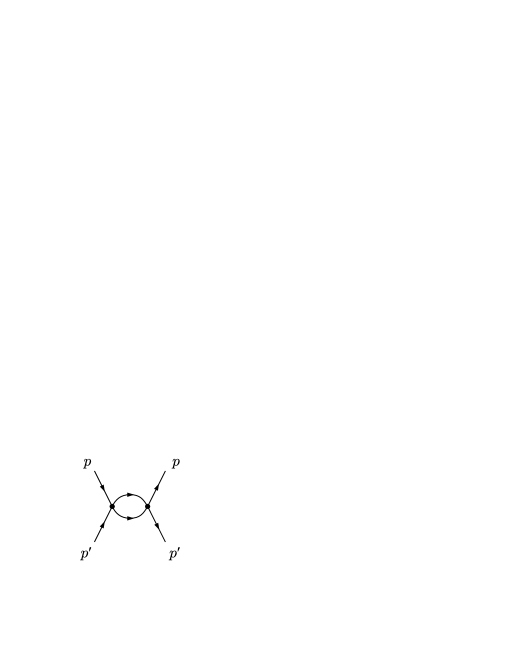
(a) s-channel

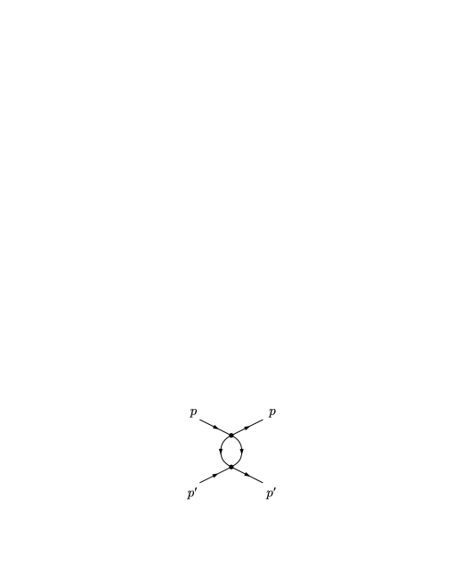
(b) t-channel

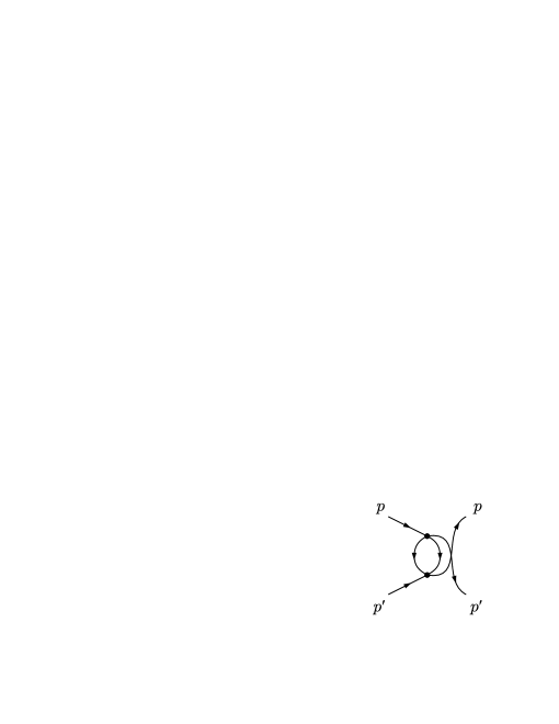
(c) u-channel

Figure 1: One-loop graphs. The basic structure for $s$, $t$ and $u$ channel graphs.

6 Two-loop amplitudes

In this section we compute the two-loop amplitudes for various four-point processes and show that there is complete agreement with the S-matrix results in Sec. 4. One consequence of the structure of the S-matrix is that the two-loop amplitudes should be related to the tree amplitudes by a universal factor $\gamma^{2}F(p_{-},p_{-}^{\prime})$, which we will explicitly show.

In order to obtain the S-matrix, one must take into account the wave-function renormalization of the external legs as well as a Jacobian factor that arises when converting $\delta$-functions for overall conservation of energy and momentum to $\delta$-functions for individual momenta. Moreover, there is a two-loop contribution to this Jacobian due to the two-loop mass-shift. The contributions from the wave-function renormalization and Jacobian will cancel off against certain terms in the amplitude to give very compact expressions for the S-matrix.

Since all interaction terms in (2.1) are four-point, the general structure for the two-loop Feynman diagrams have the form shown in Fig. 2. The diagrams fall into the 3 general classes, “double bubble”, “wineglass” and “inverse wineglass” for each of the $s$, $t$ and $u$ channels. The bosonic vertices all come with two powers of $p_{-}$, a vertex with two bosons and two fermions has one power of $p_{-}$, while the four-fermion vertex has no powers of momenta. The fermion propagator also comes with a factor of $p_{-}$, therefore the amplitudes will all have world-sheet spin $-6$. Naive power counting might indicate that these diagrams are divergent, however the two-dimensional Lorentz invariance of the free theory insures that these divergences are not there.

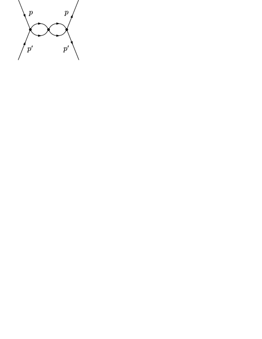
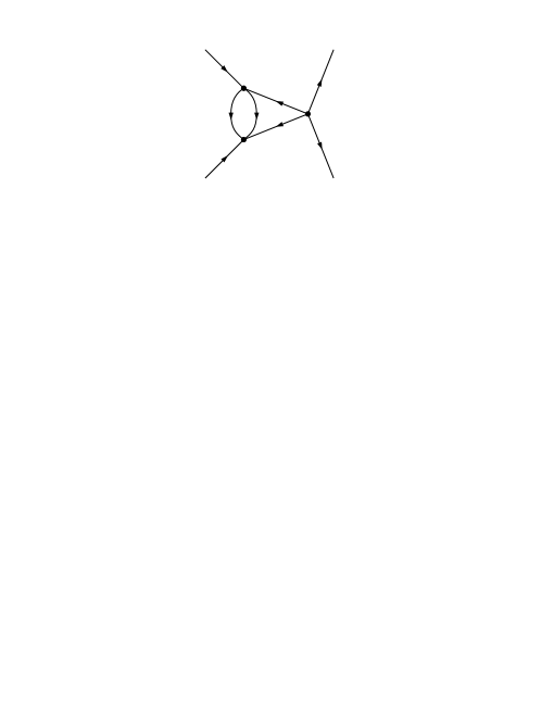
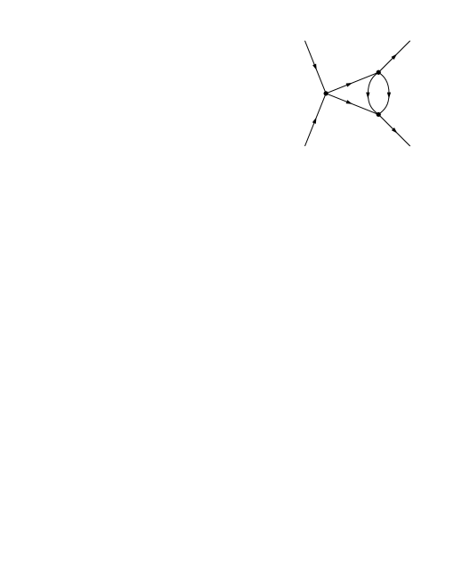
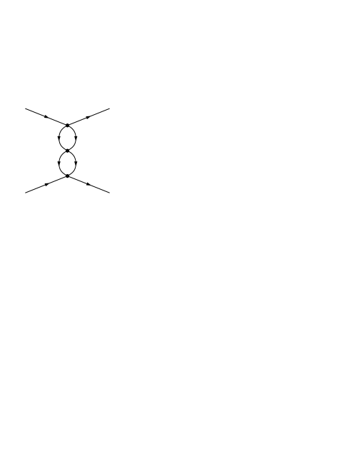
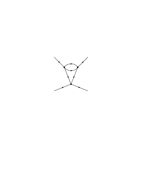
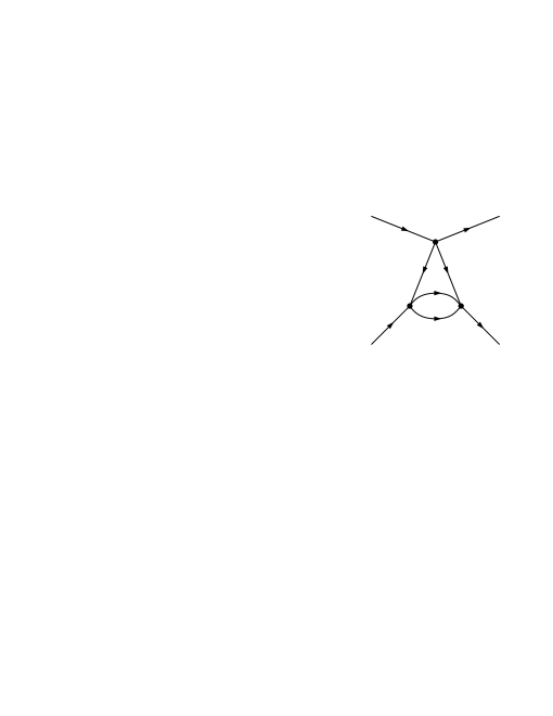
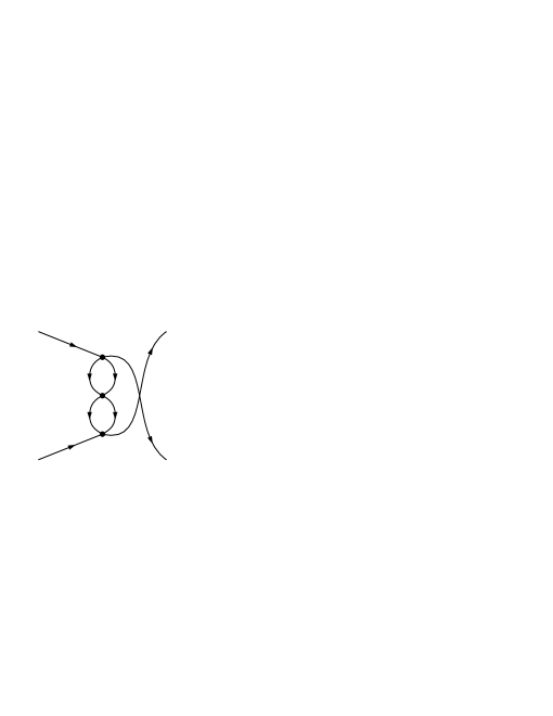
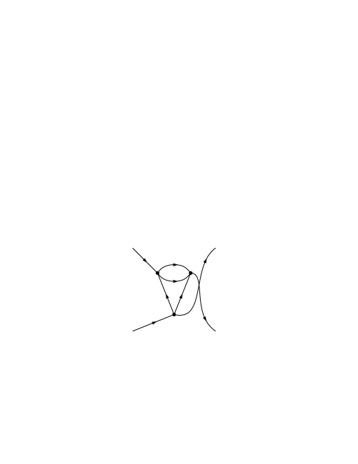
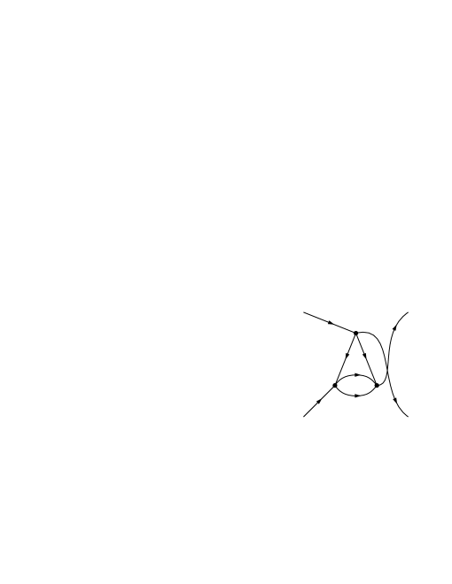
Figure 2: Two-loop graphs. The first line shows the $s$-channel diagrams, the second line the $t$-channel and the last $u$-channel. To the diagrams in the first column, we refer to as “double bubble”, to the second column as “wineglass” and to the third as “inverse wineglass”.

Let us start with the easiest set of diagrams to evaluate, the $t$-channel double bubble. For these diagrams, no external momentum flows through the internal propagators. One can argue that there must be at least two powers of the internal momenta in the numerators of the two-loop integrals, which by the Lorentz invariance of the free theory, must be zero, and so the $t$-channel bubbles all have $\mathcal{A}^{\mathrm{bubble}}_{t}(p,p^{\prime})=0$.

The next set of diagrams we consider are the $u$ and $s$ channel double bubbles. Different processes have different combinatoric factors contributing to the loop integrals, but their final results all reduce to the same form, with the $u$-channel given by

$$\mathcal{A}^{\mathrm{bubble}}_{u}(p,p^{\prime})=\gamma^{2}\mathcal{A}^{(0)}(p_{-},p_{-}^{\prime})\,F^{\mathrm{bubble}}(p_{-},p_{-}^{\prime})\;,$$ (6.1)

where $\mathcal{A}^{(0)}(p_{-},p_{-}^{\prime})$ is the tree-level amplitude for the corresponding process and

$$F^{\mathrm{bubble}}(p_{-},p_{-}^{\prime})=-\bigl{[}2(p^{\prime}_{-}-p_{-})^{2}I_{00}(p_{-},p_{-}^{\prime})\bigr{]}^{2}\;.$$ (6.2)

$I_{rs}(p_{-},p_{-}^{\prime})$ is the one-loop $u$-channel integral defined in (B.1). The $s$-channel can be obtained easily from the $u$-channel result by continuing $p_{-}^{\prime}\rightarrow-p_{-}^{\prime}$ in $F^{\mathrm{bubble}}(p_{-},p_{-}^{\prime})$, but not in $\mathcal{A}^{(0)}(p_{-},p_{-}^{\prime})$, resulting in

$$\mathcal{A}^{\mathrm{bubble}}_{s}(p_{-},p_{-}^{\prime})=\gamma^{2}\mathcal{A}^{(0)}(p_{-},p_{-}^{\prime})\,F^{\mathrm{bubble}}(p_{-},-p_{-}^{\prime})\;.$$ (6.3)

Combining the double bubbles together and substituting the expression for $I_{00}(p_{-},p_{-}^{\prime})$ in (B.2), results in

$$\begin{split}\mathcal{A}_{stu}^{\mathrm{bubbles}}=\ \gamma^{2}\mathcal{A}^{(0)}(p_{-},p_{-}^{\prime})\Biggl{[}&-\frac{p_{-}^{2}p_{-}^{\prime 2}(p_{-}^{\prime}+p_{-})^{2}}{(p_{-}^{\prime}-p_{-})^{2}}-\frac{2ip_{-}^{2}p_{-}^{\prime 2}(p_{-}^{\prime}+p_{-})^{2}}{\pi(p_{-}^{\prime}-p_{-})^{2}}\ln\frac{p_{-}^{\prime}}{p_{-}}\\ &+\frac{2p_{-}^{2}p_{-}^{\prime 2}(p_{-}^{4}+6p_{-}^{2}p_{-}^{\prime 2}+p_{-}^{\prime 4})}{\pi^{2}(p_{-}^{\prime 2}-p_{-}^{2})^{2}}\ln^{2}\frac{p_{-}^{\prime}}{p_{-}}\Biggr{]}\;.\end{split}$$ (6.4)

The wineglass diagrams are computationally more challenging because their loop integrals do not factorize into products of one-loop integrals. Nevertheless we are able to obtain compact expressions for these as well. Like the double bubble diagrams, all $2\rightarrow 2$ processes have the same proportionality factor to their tree level amplitude. For the $u$-channel wineglass, we find the expression

$$\mathcal{A}_{u}^{\mathrm{wine}}(p,p^{\prime})=16\gamma^{2}\mathcal{A}^{(0)}(p_{-},p_{-}^{\prime})\,F^{\mathrm{wine}}(p_{-},p_{-}^{\prime})\;,$$ (6.5)

where

$$\begin{split}F^{\mathrm{wine}}(p_{-},p_{-}^{\prime})=16\Bigl{[}&-4p_{-}^{2}p_{-}^{\prime 2}\,W_{0}(p_{-},p_{-}^{\prime})+8p_{-}p_{-}^{\prime}(p_{-}^{\prime}+p_{-})\,W_{1}(p_{-},p_{-}^{\prime})\\ &-(p_{-}^{2}+6p_{-}p_{-}^{\prime}+p_{-}^{\prime 2})\,W_{2}(p_{-},p_{-}^{\prime})\Bigr{]}\;.\end{split}$$ (6.6)

The wineglass integrals $W_{r}(p_{-},p_{-}^{\prime})$ are defined and discussed in App. B.3. Different processes have very different combinations to reach this same final form in (6.5) and (6.6). The $s$-channel wineglass is again related to the $u$-channel form by analytically continuing $p^{\prime}\to-p^{\prime}$ in $F^{\mathrm{wine}}(p_{-},p_{-}^{\prime})$,

$$\mathcal{A}_{s}^{\mathrm{wine}}(p,p^{\prime})=\gamma^{2}\mathcal{A}^{(0)}(p_{-},p_{-}^{\prime})\,F^{\mathrm{wine}}(p_{-},-p_{-}^{\prime})\;.$$ (6.7)

Likewise, we also find that the $t$-channel wineglass has a simple relation to the other wineglass diagrams, namely we simply set $p_{-}^{\prime}=p_{-}$ in $F^{\mathrm{wine}}(p_{-},p_{-}^{\prime})$, giving us

$$\mathcal{A}_{t}^{\mathrm{wine}}(p,p^{\prime})=\gamma^{2}\mathcal{A}^{(0)}(p_{-},p_{-}^{\prime})\,F^{\mathrm{wine}}(p_{-},p_{-})\;.$$ (6.8)

For the inverse wineglass diagrams, it is straightforward to show by the symmetries in the diagrams that

$$\mathcal{A}_{u}^{\mathrm{inverse}}(p_{-},p_{-}^{\prime})\mathrel{} = \mathrel{}\mathcal{A}_{u}^{\mathrm{wine}}(p_{-},p_{-}^{\prime})\;,$$

$$\mathcal{A}_{s}^{\mathrm{inverse}}(p_{-},p_{-}^{\prime})\mathrel{} = \mathrel{}\mathcal{A}_{s}^{\mathrm{wine}}(p_{-},p_{-}^{\prime})\;,$$ (6.9)

while the $t$-channel inverse wineglass is

$$\mathcal{A}_{t}^{\mathrm{inverse}}(p,p^{\prime})=\gamma^{2}\mathcal{A}^{(0)}(p_{-},p_{-}^{\prime})\,F^{\mathrm{wine}}(p_{-}^{\prime},p_{-}^{\prime})\;.$$ (6.10)

Putting together the terms in (6.5), (6.7) and (6) and also using (6.6) and the expressions for $W_{r}(p_{-},p_{-}^{\prime})$ in App. B.3 , we obtain the combined $su$ wineglass

$$\begin{split}\mathcal{A}_{su}^{\mathrm{wineglasses}}=\ \gamma^{2}\mathcal{A}^{(0)}(p_{-},p_{-}^{\prime})\Biggl{[}&-p_{-}^{2}p_{-}^{\prime 2}+\frac{8i\,p_{-}^{3}p_{-}^{\prime 3}}{\pi(p_{-}^{\prime 2}-p_{-}^{2})}+\frac{2ip_{-}^{2}p_{-}^{\prime 2}(p_{-}^{4}+6p_{-}^{2}p_{-}^{\prime 2}+p_{-}^{\prime 4})}{\pi(p_{-}^{\prime 2}-p_{-}^{2})^{2}}\ln\frac{p_{-}^{\prime}}{p_{-}}\\ &-\frac{2p_{-}^{2}p_{-}^{\prime 2}(p_{-}^{4}+6p_{-}^{2}p_{-}^{\prime 2}+p_{-}^{\prime 4})}{\pi^{2}(p_{-}^{\prime 2}-p_{-}^{2})^{2}}\ln^{2}\frac{p_{-}^{\prime}}{p_{-}}\Biggr{]}\;.\end{split}$$ (6.11)

Combining the $t$-channel wineglass with its inverse gives

$$\mathcal{A}_{t}^{\mathrm{wineglasses}}=\ \gamma^{2}\mathcal{A}^{(0)}(p_{-},p_{-}^{\prime})\biggl{[}\left(\frac{1}{\pi^{2}}-\frac{1}{12}\right)(p_{-}^{\prime 4}+p_{-}^{4})\biggr{]}\;,$$ (6.12)

and then combining this with (6.4) and (6.11), we reach the final two-loop amplitude

$$\mathcal{A}^{(2)}(p_{-},p_{-}^{\prime})\mathrel{} = \mathrel{}\mathcal{A}_{stu}^{\mathrm{bubbles}}(p_{-},p_{-}^{\prime})+\mathcal{A}_{su}^{\mathrm{wineglasses}}(p_{-},p_{-}^{\prime})+\mathcal{A}_{t}^{\mathrm{wineglasses}}(p_{-},p_{-}^{\prime})$$ (6.13)

$$= \mathrel{}\gamma^{2}\mathcal{A}^{(0)}(p_{-},p_{-}^{\prime})\Biggl{[}-\frac{p_{-}^{2}p_{-}^{\prime 2}(p_{-}^{\prime}+p_{-})^{2}}{(p_{-}^{\prime}-p_{-})^{2}}+\frac{8ip_{-}^{3}p_{-}^{\prime 3}}{\pi(p_{-}^{\prime 2}-p_{-}^{2})}\biggl{(}1-\frac{p_{-}^{\prime 2}+p_{-}^{2}}{p_{-}^{\prime 2}-p_{-}^{2}}\ln\frac{p_{-}^{\prime}}{p_{-}}\biggr{)}$$

$$\qquad\qquad\qquad\qquad-p_{-}^{2}p_{-}^{\prime 2}+\biggl{(}\frac{1}{\pi^{2}}-\frac{1}{12}\biggr{)}(p_{-}^{\prime 4}+p_{-}^{4})\Biggr{]}\;.$$

One should immediately note that the $(\ln\frac{p_{-}^{\prime}}{p_{-}})^{2}$ terms that appear in (6.4) and (6.11), but which are absent in the two-loop S-matrix in (4,4.13) have canceled off in the final amplitude! One can also easily see that the first line of (6.13) has precisely the right form as (4.14). The first term in the second line is accounted for by a Jacobian factor, while the second term in this line, which is due entirely to the $t$-channel contributions, is compensated by wave-function renormalization of the external legs. In fact, the renormalization of the legs with momentum $p$ through them cancels off with the $t$-wineglass, while the renormalization of the $p^{\prime}$ legs cancels against the inverse $t$-wineglass.

The Jacobian arises because the amplitudes come with factors of $\delta^{2}(P^{\mu}_{\mathrm{out}}-P^{\mu}_{\mathrm{in}})$, while the S-matrix is written with factors of $\delta(p_{-}-q_{-})\delta(p_{-}^{\prime}-q_{-}^{\prime})$. These are related by

$$\delta^{2}(P^{\mu}_{\mathrm{out}}-P^{\mu}_{\mathrm{out}})=\frac{1}{2}\left(\frac{dp_{+}^{\prime}}{dp_{-}^{\prime}}-\frac{dp_{+}}{dp_{-}}\right)^{-1}\delta(p_{-}-q_{-})\delta(p_{-}^{\prime}-q_{-}^{\prime})\;.$$ (6.14)

Taking into account the two-loop dispersion relation in (3.8), we find for the Jacobian

$$\frac{1}{2}\left(\frac{dp_{+}^{\prime}}{dp_{-}^{\prime}}-\frac{dp_{+}}{dp_{-}}\right)^{-1}=\frac{2p_{-}^{2}p_{-}^{\prime 2}}{m^{2}(p_{-}^{\prime 2}-p_{-}^{2})}\biggl{[}1+\frac{\gamma^{2}}{m^{4}}p_{-}^{2}p_{-}^{\prime 2}\biggr{]}\;.$$ (6.15)

The full S-matrix has the form

$$\mathbbm{S}=\mathbbm{1}+\frac{1}{2}\left(\frac{dp_{+}^{\prime}}{dp_{-}^{\prime}}-\frac{dp_{+}}{dp_{-}}\right)^{-1}Z(p_{-})Z(p_{-}^{\prime})\,\mathcal{A}\;.$$ (6.16)

Thus, after setting $m=1$ and substituting in (6.15) and (3.9), the two-loop contribution to the S-matrix is

$$\mathbbm{S}^{(2)}=\frac{p_{-}p_{-}^{\prime}}{2(p_{-}^{\prime 2}-p_{-}^{2})}\Biggl{[}\mathcal{A}^{(2)}+\gamma^{2}\mathcal{A}^{(0)}\biggl{(}p_{-}^{2}p_{-}^{\prime 2}-\biggl{(}\frac{1}{\pi^{2}}-\frac{1}{12}\biggr{)}(p_{-}^{\prime 4}+p_{-}^{4})\biggr{)}\Biggr{]}$$ (6.17)

Using the result for $\mathcal{A}^{(2)}$ in (6.13), we reach the final expression

$$\mathbbm{S}^{(2)}=\gamma^{2}\mathcal{A}^{(0)}\frac{p_{-}^{3}p_{-}^{\prime 3}}{2(p_{-}^{\prime 2}-p_{-}^{2})}\Biggl{[}-\left(\frac{p_{-}^{\prime}+p_{-}}{p_{-}^{\prime}-p_{-}}\right)^{2}+\frac{8i}{\pi}\,\frac{p_{-}p_{-}^{\prime}}{p_{-}^{\prime 2}-p_{-}^{2}}\left(1-\frac{p_{-}^{\prime 2}+p_{-}^{2}}{p_{-}^{\prime 2}-p_{-}^{2}}\ln\frac{p_{-}^{\prime}}{p_{-}}\right)\Biggr{]}\;,$$ (6.18)

which agrees precisely with the conjectured form (4.14), since $\mathbbm{S}^{(0)}=\mathcal{A}^{(0)}\frac{p_{-}p_{-}^{\prime}}{2(p_{-}^{\prime 2}-p_{-}^{2})}$.

7 Conclusions and outlook

The sigma-model describing the super-string on $\mathrm{AdS}_{5}\times S^{5}$ is a rather complicated theory and calculating the complete quantum S-matrix remains a formidable problem. Fortunately consideration of the near-flat space limit, as described in [22], results in significant simplifications which make loop calculations feasible. The reduced sigma-model has at most quartic interactions and the right movers essentially decouple from the interacting left-movers. Just as for the full string theory in the light-cone gauge the reduced model is not Lorentz invariant however if boosts are combined with a rescaling of the loop parameter the action is indeed invariant. This can be seen in the world-sheet S-matrix which depends only on the difference of rapidities and an effective, momentum dependent, coupling. Furthermore the simplified theory possesses at least $(0,2)$ worldsheet supersymmetry.

As an important step in the calculation of the S-matrix we computed the two-loop two point function with the corresponding mass shift and wavefunction renormalisation. This is an interesting result in its own right as we can explicitly see the modification of the relativistic dispersion by the sine function at higher powers of the momenta. In the gauge theory description the sine function arises naturally from the intrinsic discreteness of the spin-chain and indeed from the point of view of soliton description [26] the momentum is a periodic variable as it corresponds to the angular separation of the string endpoints. This is however the first case where the sine function has been seen to originate from quantum corrections to excitations about a plane-wave vacuum. Additionally in calculating the full $\mathrm{SU}(2|2)$ S-matrix we are able to check that the symmetries of the classical theory are realized at higher loop order.

Given the central role of the world-sheet S-matrix in recent developments of our understanding of the AdS/CFT correspondence it certainly interesting to extract as much information and intuition from this reduced model as possible. The spectacular agreement of our calculations with the appropriate limit of the conjectured exact S-matrix of [11],[12] provides further strong evidence in favor of its validity. It should be straightforward, though perhaps technically challenging, to extend the loop calculation to even higher orders which would provide yet further confirmation of the complete S-matrix. However, given that the theory is presumably integrable, it may be more profitable to try to find a complete solution using more non-perturbative techniques perhaps along the lines discussed in [32]. This would allow one to answer an outstanding issue not addressed by the perturbative calculation, that of the pole structure of the S-matrix. Although we consider the near-flat space limit which interpolates between the plane wave limit and the giant magnon regime we do not see the double poles of the S-matrix corresponding to exchange of BPS magnons [31]; which would require a resummation of the entire perturbative expansion.

Note added

While this paper was being prepared for publication we received [33] where the study of two-loop quantum corrections to the energies of classical string solutions was initiated.

Acknowledgments

We would like to thanks to J. Maldacena, R. Roiban and I. Swanson for discussions. The work of K.Z. was supported in part by the Swedish Research Council under contracts 621-2004-3178 and 621-2003-2742, by grant NSh-8065.2006.2 for the support of scientific schools, and by RFBR grant 06-02-17383. The work of T.K. and K.Z. was supported by the Göran Gustafsson Foundation. The work of J.A.M. was supported in part by the Swedish Research Council under contract 2006-3373. J.A.M. and T.K. thank the CTP at MIT for hospitality during the course of this work, and the STINT foundation.

Appendix A S-matrix elements

A.1 Bosons

We write the action of the T-matrix, which is defined as $\mathbbm{S}=\mathbbm{1}+\mathbbm{T}$, onto all bosonic initial states. We omit fermions in the final states. Using an $\mathrm{SO}(4)\otimes\mathrm{SO}(4)$ notation, we define the matrix elements as follows:

$$\mathbbm{T}\mathopen{|}Z_{i}Z^{\prime}_{j}\mathclose{\rangle}=\ \mathopen{|}Z_{i}Z^{\prime}_{j}\mathclose{\rangle}I_{ZZ}+\mathopen{|}Z_{j}Z^{\prime}_{i}\mathclose{\rangle}P_{ZZ}+\delta_{ij}\mathopen{|}Z_{k}Z^{\prime}_{k}\mathclose{\rangle}T_{ZZ}+\delta_{ij}\mathopen{|}Y_{k^{\prime}}Y^{\prime}_{k^{\prime}}\mathclose{\rangle}K_{ZZ}\;,$$ (A.1)

$$\mathbbm{T}\mathopen{|}Z_{i}Y^{\prime}_{j^{\prime}}\mathclose{\rangle}=\ \mathopen{|}Z_{i}Y^{\prime}_{j^{\prime}}\mathclose{\rangle}I_{ZY}+\mathopen{|}Y_{j^{\prime}}Z^{\prime}_{i}\mathclose{\rangle}P_{ZY}\;,$$ (A.2)

$$\mathbbm{T}\mathopen{|}Y_{i^{\prime}}Z^{\prime}_{j}\mathclose{\rangle}=\ \mathopen{|}Y_{i^{\prime}}Z^{\prime}_{j}\mathclose{\rangle}I_{YZ}+\mathopen{|}Z_{j}Y^{\prime}_{i^{\prime}}\mathclose{\rangle}P_{YZ}\;,$$ (A.3)

$$\mathbbm{T}\mathopen{|}Y_{i^{\prime}}Y^{\prime}_{j^{\prime}}\mathclose{\rangle}=\ \mathopen{|}Y_{i^{\prime}}Y^{\prime}_{j^{\prime}}\mathclose{\rangle}I_{YY}+\mathopen{|}Y_{j^{\prime}}Y^{\prime}_{i^{\prime}}\mathclose{\rangle}P_{YY}+\delta_{i^{\prime}j^{\prime}}\mathopen{|}Y_{k^{\prime}}Y^{\prime}_{k^{\prime}}\mathclose{\rangle}T_{YY}+\delta_{i^{\prime}j^{\prime}}\mathopen{|}Z_{k}Z^{\prime}_{k}\mathclose{\rangle}K_{YY}$$ (A.4)

The world-sheet computation yields

$$I_{ZZ}^{(0)} =-I_{YY}^{(0)}=-2i\gamma\,\frac{p_{-}p_{-}^{\prime}(p_{-}^{\prime 2}+p_{-}^{2})}{p_{-}^{\prime 2}-p_{-}^{2}}$$

$$P_{ZZ}^{(0)} =-P_{YY}^{(0)}=-4i\gamma\,\frac{p_{-}^{2}p_{-}^{\prime 2}}{p_{-}^{\prime 2}-p_{-}^{2}}$$

$$T_{ZZ}^{(0)} =-T_{YY}^{(0)}=+4i\gamma\,\frac{p_{-}^{2}p_{-}^{\prime 2}}{p_{-}^{\prime 2}-p_{-}^{2}}$$

$$K_{ZZ}^{(0)} =-K_{YY}^{(0)}=0$$

$$I_{ZZ}^{(1)} =+I_{YY}^{(1)}=-2\gamma^{2}\,\frac{p_{-}^{2}p_{-}^{\prime 2}(p_{-}^{\prime 2}+p_{-}^{2})}{(p_{-}^{\prime}-p_{-})^{2}}+\frac{8i\gamma^{2}}{\pi}\,\frac{p_{-}^{3}p_{-}^{\prime 3}}{p_{-}^{\prime 2}-p_{-}^{2}}\left(1-\frac{p_{-}^{\prime 2}+p_{-}^{2}}{p_{-}^{\prime 2}-p_{-}^{2}}\ln\frac{p_{-}^{\prime}}{p_{-}}\right)$$

$$P_{ZZ}^{(1)} =+P_{YY}^{(1)}=-4\gamma^{2}\,\frac{p_{-}^{3}p_{-}^{\prime 3}}{(p_{-}^{\prime}-p_{-})^{2}}$$

$$T_{ZZ}^{(1)} =+T_{YY}^{(1)}=+4\gamma^{2}\,\frac{p_{-}^{3}p_{-}^{\prime 3}}{(p_{-}^{\prime}+p_{-})^{2}}$$

$$K_{ZZ}^{(1)} =+K_{YY}^{(1)}=-4\gamma^{2}\,\frac{p_{-}^{3}p_{-}^{\prime 3}}{(p_{-}^{\prime}+p_{-})^{2}}$$

$$I_{ZZ}^{(2)} =-I_{YY}^{(2)}=+2i\gamma^{3}\,\frac{p_{-}^{3}p_{-}^{\prime 3}(p_{-}^{\prime}+p_{-})(p_{-}^{\prime 2}+p_{-}^{2})}{(p_{-}^{\prime}-p_{-})^{3}}+\frac{16\gamma^{3}}{\pi}\,\frac{p_{-}^{4}p_{-}^{\prime 4}(p_{-}^{\prime 2}+p_{-}^{2})}{(p_{-}^{\prime 2}-p_{-}^{2})^{2}}\left(1-\frac{p_{-}^{\prime 2}+p_{-}^{2}}{p_{-}^{\prime 2}-p_{-}^{2}}\ln\frac{p_{-}^{\prime}}{p_{-}}\right)$$

$$P_{ZZ}^{(2)} =-P_{YY}^{(2)}=+4i\gamma^{3}\,\frac{p_{-}^{4}p_{-}^{\prime 4}(p_{-}^{\prime}+p_{-})}{(p_{-}^{\prime}-p_{-})^{3}}+\frac{32\gamma^{3}}{\pi}\,\frac{p_{-}^{5}p_{-}^{\prime 5}}{(p_{-}^{\prime 2}-p_{-}^{2})^{2}}\left(1-\frac{p_{-}^{\prime 2}+p_{-}^{2}}{p_{-}^{\prime 2}-p_{-}^{2}}\ln\frac{p_{-}^{\prime}}{p_{-}}\right)$$

$$T_{ZZ}^{(2)} =-T_{YY}^{(2)}=-4i\gamma^{3}\,\frac{p_{-}^{4}p_{-}^{\prime 4}(p_{-}^{\prime}+p_{-})}{(p_{-}^{\prime}-p_{-})^{3}}-\frac{32\gamma^{3}}{\pi}\,\frac{p_{-}^{5}p_{-}^{\prime 5}}{(p_{-}^{\prime 2}-p_{-}^{2})^{2}}\left(1-\frac{p_{-}^{\prime 2}+p_{-}^{2}}{p_{-}^{\prime 2}-p_{-}^{2}}\ln\frac{p_{-}^{\prime}}{p_{-}}\right)$$

$$K_{ZZ}^{(2)} =-K_{YY}^{(2)}=0$$

$$I_{ZY}^{(0)} =-I_{YZ}^{(0)}=-2i\gamma\,p_{-}p_{-}^{\prime}$$

$$P_{ZY}^{(0)} =-P_{ZY}^{(0)}=0$$

$$I_{ZY}^{(1)} =+I_{YZ}^{(1)}=-2\gamma^{2}\,\frac{p_{-}^{2}p_{-}^{\prime 2}(p_{-}^{\prime 2}+p_{-}^{2})}{(p_{-}^{\prime}-p_{-})^{2}}+\frac{8i\gamma^{2}}{\pi}\frac{p_{-}^{3}p_{-}^{\prime 3}}{p_{-}^{\prime 2}-p_{-}^{2}}\left(1-\frac{p_{-}^{\prime 2}+p_{-}^{2}}{p_{-}^{\prime 2}-p_{-}^{2}}\ln\frac{p_{-}^{\prime}}{p_{-}}\right)$$

$$P_{ZY}^{(1)} =+P_{YZ}^{(1)}=-4\gamma^{2}\,\frac{p_{-}^{3}p_{-}^{\prime 3}}{(p_{-}^{\prime}-p_{-})^{2}}$$

$$I_{ZY}^{(2)} =-I_{YZ}^{(2)}=+2i\gamma^{3}\,\frac{p_{-}^{3}p_{-}^{\prime 3}(p_{-}^{\prime}+p_{-})^{2}}{(p_{-}^{\prime}-p_{-})^{2}}+\frac{16\gamma^{3}}{\pi}\,\frac{p_{-}^{4}p_{-}^{\prime 4}}{p_{-}^{\prime 2}-p_{-}^{2}}\left(1-\frac{p_{-}^{\prime 2}+p_{-}^{2}}{p_{-}^{\prime 2}-p_{-}^{2}}\ln\frac{p_{-}^{\prime}}{p_{-}}\right)$$

$$P_{ZY}^{(2)} =-P_{YZ}^{(2)}=0$$

These coefficients have to be compared to the S-matrix elements (4.13) in the follow way:

$$1+I_{YY} =S_{0}\,A\,(A+B)\;, 1+I_{ZZ} =S_{0}\,D\,(D+E)\;,$$ (A.5)

$$P_{YY} =S_{0}\,B\,(A+B)\;, P_{ZZ} =S_{0}\,E\,(D+E)\;,$$

$$T_{YY} =-S_{0}\,A\,B\;, T_{ZZ} =-S_{0}\,D\,E\;,$$

$$K_{YY} =-S_{0}\,C^{2}\;, K_{ZZ} =-S_{0}\,F^{2}\;,$$

$$1+I_{ZY} =S_{0}\,L^{2}\;, 1+I_{YZ} =S_{0}\,G^{2}\;,$$

$$P_{ZY} =S_{0}\,K^{2}\;, P_{YZ} =S_{0}\,H^{2}\;.$$

Here $S_{0}$ denotes the prefactor in (4.9). We find perfect agreement. Note that we are sensitive to all matrix elements, even though we concentrate onto the scattering among bosons. This is because the field $Z$ actually carries two fermionic indices in the $\mathfrak{su}(2|2)^{2}$ notation.

A.2 $\mathrm{SU}(2|2)$ subsector

We now extend our considerations to include processes involving fermions, however, we restrict ourselves to a single $\mathfrak{su}(2|2)$ sector. Granting the group factorization of the full S-matrix, this is a sufficient test of the supersymmetries at higher loop orders.

As described in App. C, we identify in the worldsheet theory the fields $\phi_{a}$ and $\chi_{\alpha}$ spanning an $\mathfrak{su}(2|2)$ sector. We calculate the matrix elements defined as follows:

$$\mathbbm{S}\mathopen{|}\phi_{a}\phi^{\prime}_{b}\mathclose{\rangle} ={\cal S}_{0}{\cal{A}}\mathopen{|}\phi_{a}\phi^{\prime}_{b}\mathclose{\rangle}+{\cal S}_{0}{\cal{B}}\mathopen{|}\phi_{b}\phi^{\prime}_{a}\mathclose{\rangle}+{\cal S}_{0}{\cal{C}}\varepsilon_{ab}\varepsilon^{\alpha\beta}\mathopen{|}\chi_{\alpha}\chi^{\prime}_{\beta}\mathclose{\rangle}\;,$$ (A.6)

$$\mathbbm{S}\mathopen{|}\chi_{\alpha}\chi^{\prime}_{\beta}\mathclose{\rangle} ={\cal S}_{0}{\cal{D}}\mathopen{|}\chi_{\alpha}\chi^{\prime}_{\beta}\mathclose{\rangle}+{\cal S}_{0}{\cal{E}}\mathopen{|}\chi_{\beta}\chi^{\prime}_{\alpha}\mathclose{\rangle}+{\cal S}_{0}{\cal{F}}\varepsilon_{\alpha\beta}\varepsilon^{ab}\mathopen{|}\phi_{a}\phi^{\prime}_{b}\mathclose{\rangle}\;,$$ (A.7)

$$\mathbbm{S}\mathopen{|}\phi_{a}\chi^{\prime}_{\beta}\mathclose{\rangle} ={\cal S}_{0}{\cal{G}}\mathopen{|}\phi_{a}\chi^{\prime}_{\beta}\mathclose{\rangle}+{\cal S}_{0}{\cal{H}}\mathopen{|}\chi_{\beta}\phi^{\prime}_{a}\mathclose{\rangle}\;,$$ (A.8)

$$\mathbbm{S}\mathopen{|}\chi_{\alpha}\phi^{\prime}_{b}\mathclose{\rangle} ={\cal S}_{0}{\cal{K}}\mathopen{|}\phi_{b}\chi^{\prime}_{\alpha}\mathclose{\rangle}+{\cal S}_{0}{\cal{L}}\mathopen{|}\chi_{\alpha}\phi^{\prime}_{b}\mathclose{\rangle}\;.$$ (A.9)

For the sake of brevity we will not record the individual amplitudes but simply state the final results for the ${S}$-matrix elements, noting that they agree with the all-order prediction from the dual spin chain description. There is a common contribution to each element of the form ${\cal S}_{0}=1+i\delta$ where

$$\delta=\frac{8\gamma}{\pi}\frac{p_{-}^{3}p_{-}^{\prime 3}}{p_{-}^{\prime 2}-p_{-}^{2}}\left(1-\frac{p_{-}^{\prime 2}+p_{-}^{2}}{p_{-}^{\prime 2}-p_{-}^{2}}\ln\frac{p_{-}^{\prime}}{p_{-}}\right)$$ (A.10)

in addition to the individual contributions

$${\cal{A}} = 1+2i\gamma\,\frac{p_{-}p_{-}^{\prime}(p_{-}^{2}+p_{-}^{\prime 2})}{p_{-}^{\prime 2}-p_{-}^{2}}-2\gamma^{2}\,\frac{p_{-}^{2}p_{-}^{\prime 2}(p_{-}^{2}+p_{-}^{\prime 2})}{(p_{-}^{\prime}-p_{-})^{2}}+2i\gamma^{3}\,\frac{p_{-}^{3}p_{-}^{\prime 3}(p_{-}^{3}+p_{-}^{2}p_{-}^{\prime}+p_{-}p_{-}^{\prime 2}+p_{-}^{\prime 3})}{(p_{-}^{\prime}-p_{-})^{3}}$$

$${\cal{B}} = -{E}=4i\gamma\,\frac{p_{-}^{2}p_{-}^{\prime 2}}{p_{-}^{\prime 2}-p_{-}^{2}}-4\gamma^{2}\,\frac{p_{-}^{3}p_{-}^{\prime 3}}{(p_{-}^{\prime}-p_{-})^{2}}-4i\gamma^{3}\,\frac{p_{-}^{4}p_{-}^{\prime 4}(p_{-}+p_{-}^{\prime})}{(p_{-}^{\prime}-p_{-})^{3}}$$

$${\cal{C}} = {\cal{F}}=2i\gamma\,\frac{(p_{-}p_{-}^{\prime})^{\frac{3}{2}}}{p_{-}^{\prime}+p_{-}}-2\gamma^{2}\,\frac{(p_{-}p_{-}^{\prime})^{\frac{5}{2}}}{(p_{-}^{\prime}-p_{-})}-2i\gamma^{3}\,\frac{(p_{-}p_{-}^{\prime})^{\frac{7}{2}}(p_{-}+p_{-}^{\prime})}{(p_{-}^{\prime}-p_{-})^{2}}$$

$${\cal{D}} = 1+4i\gamma\,\frac{p_{-}^{2}p_{-}^{\prime 2}}{p_{-}^{\prime 2}-p_{-}^{2}}-4\gamma^{2}\,\frac{p_{-}^{3}p_{-}^{\prime 3}}{(p_{-}^{\prime}-p_{-})^{2}}-4i\gamma^{3}\,\frac{p_{-}^{4}p_{-}^{\prime 4}(p_{-}+p_{-}^{\prime})}{(p_{-}^{\prime}-p_{-})^{3}}$$

$${\cal{G}} = 1+2i\gamma\,\frac{p_{-}p_{-}^{\prime 2}}{p_{-}^{\prime}-p_{-}}-2\gamma^{2}\,\frac{p_{-}^{2}p_{-}^{\prime 3}(p_{-}+p_{-}^{\prime})}{(p_{-}^{\prime}-p_{-})^{2}}-2i\gamma^{3}\,\frac{p_{-}^{3}p_{-}^{\prime 4}(p_{-}+p_{-})^{2}}{(p_{-}^{\prime}-p_{-})^{3}}$$

$${\cal{H}} = {\cal{K}}=2i\gamma\,\frac{(p_{-}p_{-}^{\prime})^{\frac{3}{2}}}{p_{-}^{\prime}-p_{-}}+2\gamma^{2}\,\frac{(p_{-}p_{-}^{\prime})^{\frac{5}{2}}(p_{-}+p_{-}^{\prime})}{(p_{-}^{\prime}-p_{-})^{2}}-2i\gamma^{3}\,\frac{(p_{-}p_{-}^{\prime})^{\frac{7}{2}}(p_{-}+p_{-}^{\prime})^{2}}{(p_{-}^{\prime}-p_{-})^{3}}$$

$${\cal{L}} = 1+2i\gamma\,\frac{p_{-}^{2}p_{-}^{\prime}}{p_{-}^{\prime}-p_{-}}-2\gamma^{2}\,\frac{p_{-}^{3}p_{-}^{\prime 2}(p_{-}+p_{-}^{\prime})}{(p_{-}^{\prime}-p_{-})^{2}}-2i\gamma^{3}\,\frac{p_{-}^{4}p_{-}^{\prime 3}(p_{-}+p_{-})^{2}}{(p_{-}^{\prime}-p_{-})^{3}}\ .$$

In considering a single $\mathrm{SU}(2|2)$ sector the full S-matrix is

$$\mathbbm{S}=S_{0}\,{S}\otimes({A}+{B})$$ (A.11)

as one index in the tensor product is kept fixed by the scattering. Thus we can write these elements in a simple compact form in terms of the S-matrix defined in 4,

$$\mathbbm{S}=\frac{e^{i\delta}}{1-i\gamma p_{-}p_{-}^{\prime}\frac{p_{-}^{\prime}+p_{-}}{p_{-}^{\prime}-p_{-}}}\ {S}\otimes\mathbbm{1}\;,$$ (A.12)

and which of course is in agreement with the AdS/CFT prediction to this order. Thus we see that the symmetries are preserved to at least two-loops in the reduced sigma model.

Appendix B Integrals

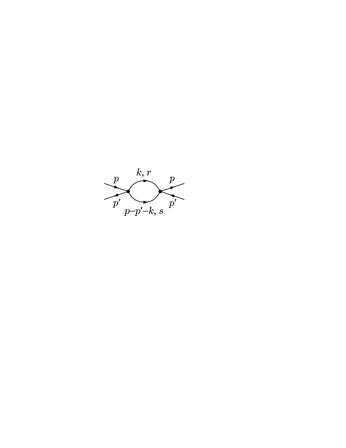
(a) bubble

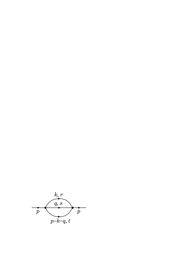
(b) sunset

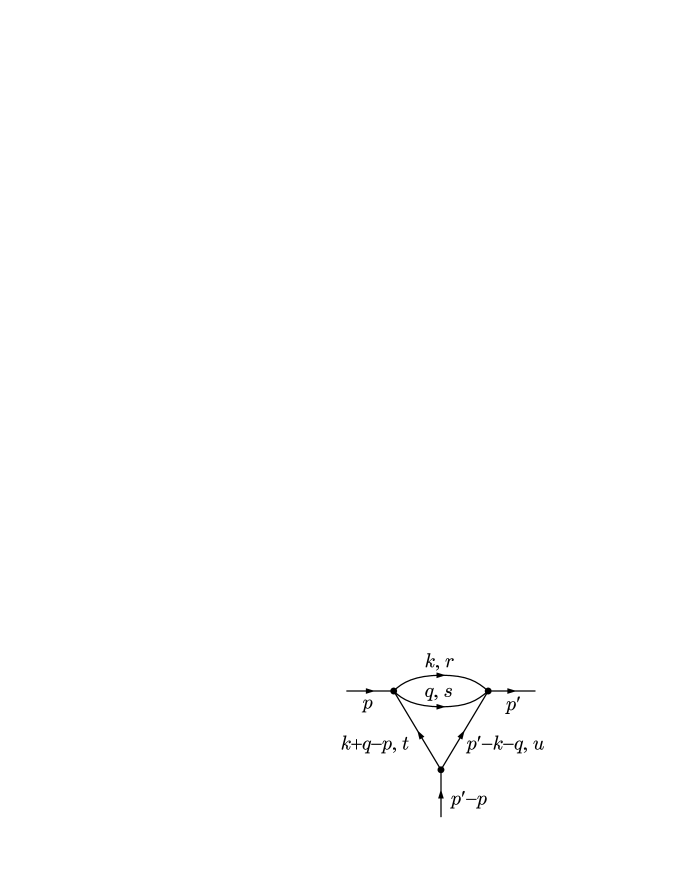
(c) wineglass

Figure 3: Loop diagrams

B.1 Bubble integral

We consider the bubble integral, cf. Fig. 3(a), for two inflowing momenta $p$ and $-p^{\prime}$ as appropriate for $u$-channel processes. With $r$ and $s$ powers of momentum inserted, the integral reads

$$I_{rs}(p,p^{\prime})=\int\frac{d^{2}\mathbf{k}}{(2\pi)^{2}}\frac{(k_{-})^{r}(p_{-}-p_{-}^{\prime}-k_{-})^{s}}{(\mathbf{k}^{2}-m^{2})[(\mathbf{p}-\mathbf{p}^{\prime}-\mathbf{k})^{2}-m^{2}]}\;.$$ (B.1)

These momenta originate from derivative couplings and fermionic propagators. However, it turns out that all amplitudes simplify such that we only need to explicitely compute $I_{00}$, which is immediately found to be

$$I_{00}(p,p^{\prime})=\frac{i}{2\pi m^{2}}\frac{p_{-}p_{-}^{\prime}}{p_{-}^{\prime 2}-p_{-}^{2}}\ln\frac{p_{-}^{\prime}}{p_{-}}\;.$$ (B.2)

In the $s$-channel, the inflowing momenta are $p$ and $p^{\prime}$. The integral $I_{00}(p,-p^{\prime})$ is obtained from (B.2) by analytically continuing the logarithm. In the $t$-channel, the total inflowing momentum is zero and we obtain from (B.2) in the limit $p^{\prime}\to p$:

$$I_{00}(p,p)=\frac{i}{4\pi m^{2}}\;.$$ (B.3)

B.2 Sunset integral

The general sunset diagram, Fig. 3(b), is defined as

$$I_{rst}(p)=\int\frac{d^{2}\mathbf{k}\,d^{2}\mathbf{q}}{(2\pi)^{4}}\frac{(k_{-})^{r}\,(q_{-})^{s}\,(p_{-}-k_{-}-q_{-})^{t}}{(\mathbf{k}^{2}-m^{2})(\mathbf{q}^{2}-m^{2})((\mathbf{p}-\mathbf{k}-\mathbf{q})^{2}-m^{2})}\;.$$ (B.4)

There is the relation

$$p_{-}I_{rst}=I_{r+1,s,t}+I_{r,s+1,t}+I_{r,s,t+1}$$ (B.5)

between different integrals which follows immediately from taking the $p_{-}$ on the left hand side into the integrand and writing it as $k_{-}+q_{-}+(p_{-}-k_{-}-q_{-})$. Using this identity, it is possible to reduce all sums of sunset diagrams that occur in the two-loop propagator to $I_{000}$. We solve this integral by introducing three Feynman parameters

$$I_{000}(\mathbf{p}^{2})=\frac{1}{16\pi^{2}}\int_{0}^{1}\frac{dx_{1}\,dx_{2}\,dx_{3}\;\delta(x_{1}+x_{2}+x_{3}-1)}{m^{2}(x_{1}x_{2}+x_{1}x_{3}+x_{2}x_{3})-\mathbf{p}^{2}\,x_{1}x_{2}x_{3}}\;.$$ (B.6)

Observe that this integral depends only on $\mathbf{p}^{2}$. On-shell the value of the integral is

$$I_{000}(\mathbf{p}^{2}=m^{2})=\frac{1}{64m^{2}}\;.$$ (B.7)

Apart form this, we also need the on-shell value of the first derivative of $I_{000}$ with repect to its argument, which is given by

$$\begin{split}I^{\prime}_{000}(\mathbf{p}^{2}=m^{2})&=\frac{1}{(4\pi)^{2}m^{4}}\int_{0}^{1}\frac{dx_{1}\,dx_{2}\,dx_{3}\;\delta(x_{1}+x_{2}+x_{3}-1)\,x_{1}x_{2}x_{3}}{(x_{1}x_{2}+x_{1}x_{3}+x_{2}x_{3}-x_{1}x_{2}x_{3})^{2}}\\ &=\frac{3}{64m^{4}}\left(\frac{1}{\pi^{2}}-\frac{1}{12}\right)\;.\end{split}$$ (B.8)

B.3 Wineglass integral

The wineglass diagram as drawn in Fig. 3(c) reads

$$W_{rstu}(p,p^{\prime})=\int\frac{d^{2}\mathbf{k}\,d^{2}\mathbf{q}}{(2\pi)^{4}}\,\frac{(k_{-})^{n_{1}}(q_{-})^{n_{2}}(k_{-}+q_{-}-p_{-})^{n_{3}}(p^{\prime}_{-}-k_{-}-q_{-})^{n_{4}}}{(\mathbf{k}^{2}-m^{2})(\mathbf{q}^{2}-m^{2})[(\mathbf{k}+\mathbf{q}-\mathbf{p})^{2}-m^{2}][(\mathbf{p}^{\prime}-\mathbf{k}-\mathbf{q})^{2}-m^{2}]}\;.$$ (B.9)

We note the identities

$$W_{rstu}(p,p^{\prime})=W_{srtu}(p,p^{\prime})=(-1)^{t+u}W_{rsut}(p^{\prime},p)=(-1)^{r+s+t+u}W_{rstu}(-p,-p^{\prime})\;.$$ (B.10)

All sums of wineglass integrals that occur in the two-loop amplitudes can be reduced to combinations of the following three terms which we compute by standard means and find

$$W_{0}(p,p^{\prime}) =W_{0000}(p,p^{\prime})$$

$$=-\frac{p_{-}p_{-}^{\prime}}{16\pi^{2}m^{4}}\left[\frac{\pi^{2}}{4(p_{-}^{\prime}+p_{-})^{2}}+\frac{1}{(p_{-}^{\prime 2}-p_{-}^{2})}\ln\frac{p_{-}^{\prime}}{p_{-}}-\frac{p_{-}p_{-}^{\prime}}{(p_{-}^{\prime 2}-p_{-}^{2})^{2}}\ln^{2}\frac{p_{-}^{\prime}}{p_{-}}\right]\;,$$ (B.11)

$$W_{1}(p,p^{\prime}) =W_{1000}(p,p^{\prime})$$

$$=-\frac{p_{-}p_{-}^{\prime}}{16\pi^{2}m^{4}}\left[\frac{\pi^{2}}{8(p_{-}^{\prime}+p_{-})}-\frac{p_{-}p_{-}^{\prime}}{2(p_{-}^{\prime}-p_{-})(p_{-}^{\prime 2}-p_{-}^{2})}\ln^{2}\frac{p_{-}^{\prime}}{p_{-}}\right]\;,$$ (B.12)

$$W_{2}(p,p^{\prime}) =W_{1100}(p,p^{\prime})+W_{2000}(p,p^{\prime})$$

$$=-\frac{p_{-}p_{-}^{\prime}}{16\pi^{2}m^{4}}\left[\frac{\pi^{2}}{12}-\frac{p_{-}p_{-}^{\prime}}{2(p_{-}^{\prime}-p_{-})^{2}}\ln^{2}\frac{p_{-}^{\prime}}{p_{-}}\right]\;.$$ (B.13)

Appendix C Notations

In this section we summarize several of the notations used throughout the main text and record several useful results. We make use of the light-cone coordinates and momenta

$$\sigma^{\pm}=\sigma^{0}\pm\sigma^{1}\quad,\quad p_{\pm}={\textstyle\frac{1}{2}}(p_{0}\pm p_{1})\;$$ (C.1)

so that the worldsheet metric is $\eta_{\mu\nu}=(+,-)$. We also use the notation $\varepsilon=p_{0}$ and $p=p_{1}$, and bold-face for world-sheet two-vectors like $\mathbf{p}=(p_{0},p_{1})$.

It is convenient to perform quantization in world-sheet light-cone coordinates with $\sigma^{+}$ as time and where the target space fields have the mode expansions

$$Z_{i}(\boldsymbol{\sigma}) =\int\frac{dp_{-}}{2\pi}\frac{1}{\sqrt{2p_{-}}}\>\Bigl{[}a_{i}(p_{-})\,e^{-i\mathbf{p}\cdot\boldsymbol{\sigma}}+a^{\dagger}_{i}(p_{-})\,e^{+i\mathbf{p}\cdot\boldsymbol{\sigma}}\Bigr{]}\;,$$ (C.2)

$$Y_{i^{\prime}}(\boldsymbol{\sigma}) =\int\frac{dp_{-}}{2\pi}\frac{1}{\sqrt{2p_{-}}}\>\Bigl{[}a_{i^{\prime}}(p_{-})\,e^{-i\mathbf{p}\cdot\boldsymbol{\sigma}}+a^{\dagger}_{i^{\prime}}(p_{-})\,e^{+i\mathbf{p}\cdot\boldsymbol{\sigma}}\Bigr{]}\;,$$ (C.3)

$$\psi(\boldsymbol{\sigma}) =\int\frac{dp_{-}}{2\pi}\frac{1}{\sqrt{2}}\>\Bigl{[}b(p_{-})\,e^{-i\mathbf{p}\cdot\boldsymbol{\sigma}}+b^{\dagger}(p_{-})\,e^{+i\mathbf{p}\cdot\boldsymbol{\sigma}}\Bigr{]}\;.$$ (C.4)

The free bosonic and fermionic propagators are

$$\frac{i}{\mathbf{p}^{2}-m^{2}}\quad,\quad\frac{ip_{-}}{\mathbf{p}^{2}-m^{2}}$$ (C.5)

and the free dispersion relation is $2p_{+}=\tfrac{m^{2}}{2p_{-}}$.

We use the following representation for the $16\times 16$ $\gamma$-matrices

$$\mathnormal{\Gamma}^{1} =\epsilon\times\epsilon\times\epsilon\times\epsilon \mathnormal{\Gamma}^{5} =\tau_{3}\times\epsilon\times\mathbbm{1}\times\epsilon$$

$$\mathnormal{\Gamma}^{2} =\mathbbm{1}\times\tau_{1}\times\epsilon\times\epsilon \mathnormal{\Gamma}^{6} =\epsilon\times\mathbbm{1}\times\tau_{1}\times\epsilon$$ (C.6)

$$\mathnormal{\Gamma}^{3} =\mathbbm{1}\times\tau_{3}\times\epsilon\times\epsilon \mathnormal{\Gamma}^{7} =\epsilon\times\mathbbm{1}\times\tau_{3}\times\epsilon$$

$$\mathnormal{\Gamma}^{4} =\tau_{1}\times\epsilon\times\mathbbm{1}\times\epsilon \mathnormal{\Gamma}^{8} =\mathbbm{1}\times\mathbbm{1}\times\mathbbm{1}\times\tau_{1}$$

with

$$\epsilon=\left(\begin{array}[]{cc}0&1\\ -1&0\end{array}\right)\quad,\quad\tau_{1}=\left(\begin{array}[]{cc}0&1\\ 1&0\end{array}\right)\quad,\quad\tau_{3}=\left(\begin{array}[]{cc}1&0\\ 0&-1\end{array}\right)\;.$$ (C.13)

We also define $\mathnormal{\Gamma}^{9}=\mathnormal{\Gamma}^{1}\mathnormal{\Gamma}^{2}\cdots\mathnormal{\Gamma}^{8}$ and $P_{L,R}={\textstyle\frac{1}{2}}(\mathbbm{1}\pm\mathnormal{\Gamma}^{9})$. The fermion $\psi$ is a real, positive chirality spinor and hence has eight real degrees of freedom.

The $\mathfrak{su}(2|2)$ sector considered in Sec. A.2 is spanned by the bosonic fields

$$\phi_{1} =\frac{1}{\sqrt{2}}(Y_{5}+iY_{6})\;, \phi_{2} =\frac{1}{\sqrt{2}}(Y_{7}+iY_{8})\;,$$ (C.14)

and the fermionic fields, $\chi_{\alpha}$, which are most easily defined in terms of the projection operators,

$$P^{I}_{\pm} = \frac{1}{2}\left(\mathbbm{1}\pm\mathnormal{\Gamma}^{1}\mathnormal{\Gamma}^{2}\mathnormal{\Gamma}^{3}\mathnormal{\Gamma}^{4}\right)$$

$$P^{II}_{\pm} = \frac{1}{2}\left(\mathbbm{1}\pm\frac{i}{2}\left(\mathnormal{\Gamma}^{56}+\mathnormal{\Gamma}^{78}\right)\right)$$

$$P^{III}_{\pm} = \frac{1}{2}\left(\mathbbm{1}\pm\frac{i}{2}\left(\mathnormal{\Gamma}^{12}+\mathnormal{\Gamma}^{34}\right)\right),$$ (C.15)

such that,

$$\chi_{3} = P^{III}_{+}P^{II}_{+}P^{I}_{-}P_{L}\psi\;,$$

$$\chi_{4} = P^{III}_{-}P^{II}_{+}P^{I}_{-}P_{L}\psi\ \;.$$ (C.16)

These correspond to the fields $\phi_{a}=Y_{a\dot{1}}$ and $\chi_{\alpha}=\mathnormal{\Upsilon}_{\alpha\dot{1}}$ in the notation of [23].

Appendix D S-matrix action

We spell out the action of the S-matrix onto the entire set of two-particle states in $\mathfrak{su}(2)^{4}$ notation, cf. [24]. This serves as a reference for which processes can occur. Taking into account that the coefficients $B$, $E$, $C$, $F$, $H$, $K$ are of order $\gamma=\frac{\pi}{\sqrt{\lambda}}$, we see that some of the processes are absent at tree-level. The terms that are present at tree-level are printed in bold face. To simplify the formulas, we suppress the $S_{0}$ that multiplies all right hand sides in the following.

Boson-Boson

$$\begin{split}\mathbbm{S}\mathopen{|}Y_{{a}{\dot{a}}}Y^{\prime}_{{b}{\dot{b}}}\mathclose{\rangle}=\ &+A^{2}\,\mbox{$\mathopen{|}Y_{{a}{\dot{a}}}Y^{\prime}_{{b}{\dot{b}}}\mathclose{\rangle}$}+AB\,\mbox{$\mathopen{|}Y_{{b}{\dot{a}}}Y^{\prime}_{{a}{\dot{b}}}\mathclose{\rangle}$}+AB\,\mbox{$\mathopen{|}Y_{{a}{\dot{b}}}Y^{\prime}_{{b}{\dot{a}}}\mathclose{\rangle}$}+B^{2}\,\mathopen{|}Y_{{b}{\dot{b}}}Y^{\prime}_{{a}{\dot{a}}}\mathclose{\rangle}\\ &+AC\,\epsilon_{{a}{b}}\epsilon^{{\gamma}{\delta}}\mbox{$\mathopen{|}\mathnormal{\Upsilon}_{{\gamma}{\dot{a}}}\mathnormal{\Upsilon}^{\prime}_{{\delta}{\dot{b}}}\mathclose{\rangle}$}+BC\,\epsilon_{{a}{b}}\epsilon^{{\gamma}{\delta}}\mathopen{|}\mathnormal{\Upsilon}_{{\gamma}{\dot{b}}}\mathnormal{\Upsilon}^{\prime}_{{\delta}{\dot{a}}}\mathclose{\rangle}\\ &+AC\,\epsilon_{{\dot{a}}{\dot{b}}}\epsilon^{{\dot{\gamma}}{\dot{\delta}}}\mbox{$\mathopen{|}\mathnormal{\Psi}_{{a}{\dot{\gamma}}}\mathnormal{\Psi}^{\prime}_{{b}{\dot{\delta}}}\mathclose{\rangle}$}+BC\,\epsilon_{{\dot{a}}{\dot{b}}}\epsilon^{{\dot{\gamma}}{\dot{\delta}}}\mathopen{|}\mathnormal{\Psi}_{{b}{\dot{\gamma}}}\mathnormal{\Psi}^{\prime}_{{a}{\dot{\delta}}}\mathclose{\rangle}\\ &+C^{2}\,\epsilon_{{a}{b}}\epsilon_{{\dot{a}}{\dot{b}}}\epsilon^{{\gamma}{\delta}}\epsilon^{{\dot{\gamma}}{\dot{\delta}}}\mathopen{|}Z_{{\gamma}{\dot{\gamma}}}Z^{\prime}_{{\delta}{\dot{\delta}}}\mathclose{\rangle}\\[8.53581pt] \mathbbm{S}\mathopen{|}Z_{{\alpha}{\dot{\alpha}}}Z^{\prime}_{{\beta}{\dot{\beta}}}\mathclose{\rangle}=\ &+D^{2}\,\mbox{$\mathopen{|}Z_{{\alpha}{\dot{\alpha}}}Z^{\prime}_{{\beta}{\dot{\beta}}}\mathclose{\rangle}$}+DE\,\mbox{$\mathopen{|}Z_{{\beta}{\dot{\alpha}}}Z^{\prime}_{{\alpha}{\dot{\beta}}}\mathclose{\rangle}$}+DE\,\mbox{$\mathopen{|}Z_{{\alpha}{\dot{\beta}}}Z^{\prime}_{{\beta}{\dot{\alpha}}}\mathclose{\rangle}$}+E^{2}\,\mathopen{|}Z_{{\beta}{\dot{\beta}}}Z^{\prime}_{{\alpha}{\dot{\alpha}}}\mathclose{\rangle}\\ &+DF\,\epsilon_{{\dot{\alpha}}{\dot{\beta}}}\epsilon^{{\dot{c}}{\dot{d}}}\mbox{$\mathopen{|}\mathnormal{\Upsilon}_{{\alpha}{\dot{c}}}\mathnormal{\Upsilon}^{\prime}_{{\beta}{\dot{d}}}\mathclose{\rangle}$}+EF\,\epsilon_{{\dot{\alpha}}{\dot{\beta}}}\epsilon^{{\dot{c}}{\dot{d}}}\mathopen{|}\mathnormal{\Upsilon}_{{\beta}{\dot{c}}}\mathnormal{\Upsilon}^{\prime}_{{\alpha}{\dot{d}}}\mathclose{\rangle}\\ &+DF\,\epsilon_{{\alpha}{\beta}}\epsilon^{{c}{d}}\mbox{$\mathopen{|}\mathnormal{\Psi}_{{c}{\dot{\alpha}}}\mathnormal{\Psi}^{\prime}_{{d}{\dot{\beta}}}\mathclose{\rangle}$}+EF\,\epsilon_{{\alpha}{\beta}}\epsilon^{{c}{d}}\mathopen{|}\mathnormal{\Psi}_{{c}{\dot{\beta}}}\mathnormal{\Psi}^{\prime}_{{d}{\dot{\alpha}}}\mathclose{\rangle}\\ &+F^{2}\,\epsilon_{{\alpha}{\beta}}\epsilon_{{\dot{\alpha}}{\dot{\beta}}}\epsilon^{{c}{d}}\epsilon^{{\dot{c}}{\dot{d}}}\mathopen{|}Y_{{c}{\dot{c}}}Y^{\prime}_{{d}{\dot{d}}}\mathclose{\rangle}\\[8.53581pt] \mathbbm{S}\mathopen{|}Y_{{a}{\dot{a}}}Z^{\prime}_{{\beta}{\dot{\beta}}}\mathclose{\rangle}=\ &+G^{2}\,\mbox{$\mathopen{|}Y_{{a}{\dot{a}}}Z^{\prime}_{{\beta}{\dot{\beta}}}\mathclose{\rangle}$}+GH\,\mbox{$\mathopen{|}\mathnormal{\Upsilon}_{{\beta}{\dot{a}}}\mathnormal{\Psi}^{\prime}_{{a}{\dot{\beta}}}\mathclose{\rangle}$}+GH\,\mbox{$\mathopen{|}\mathnormal{\Psi}_{{a}{\dot{\beta}}}\mathnormal{\Upsilon}^{\prime}_{{\beta}{\dot{a}}}\mathclose{\rangle}$}+H^{2}\,\mathopen{|}Z_{{\beta}{\dot{\beta}}}Y^{\prime}_{{a}{\dot{a}}}\mathclose{\rangle}\\[8.53581pt] \mathbbm{S}\mathopen{|}Z_{{\alpha}{\dot{\alpha}}}Y^{\prime}_{{b}{\dot{b}}}\mathclose{\rangle}=\ &+L^{2}\,\mbox{$\mathopen{|}Z_{{\alpha}{\dot{\alpha}}}Y^{\prime}_{{b}{\dot{b}}}\mathclose{\rangle}$}+KL\,\mbox{$\mathopen{|}\mathnormal{\Psi}_{{b}{\dot{\alpha}}}\mathnormal{\Upsilon}^{\prime}_{{\alpha}{\dot{b}}}\mathclose{\rangle}$}+KL\,\mbox{$\mathopen{|}\mathnormal{\Upsilon}_{{\alpha}{\dot{b}}}\mathnormal{\Psi}^{\prime}_{{b}{\dot{\alpha}}}\mathclose{\rangle}$}+K^{2}\,\mathopen{|}Y_{{b}{\dot{b}}}Z^{\prime}_{{\alpha}{\dot{\alpha}}}\mathclose{\rangle}\end{split}$$

Fermion-Fermion

$$\begin{split}\mathbbm{S}\mathopen{|}\mathnormal{\Psi}_{{a}{\dot{\alpha}}}\mathnormal{\Psi}^{\prime}_{{b}{\dot{\beta}}}\mathclose{\rangle}=\ &+AD\,\mbox{$\mathopen{|}\mathnormal{\Psi}_{{a}{\dot{\alpha}}}\mathnormal{\Psi}^{\prime}_{{b}{\dot{\beta}}}\mathclose{\rangle}$}+BD\,\mbox{$\mathopen{|}\mathnormal{\Psi}_{{b}{\dot{\alpha}}}\mathnormal{\Psi}^{\prime}_{{a}{\dot{\beta}}}\mathclose{\rangle}$}+AE\,\mbox{$\mathopen{|}\mathnormal{\Psi}_{{a}{\dot{\beta}}}\mathnormal{\Psi}^{\prime}_{{b}{\dot{\alpha}}}\mathclose{\rangle}$}+BE\,\mathopen{|}\mathnormal{\Psi}_{{b}{\dot{\beta}}}\mathnormal{\Psi}^{\prime}_{{a}{\dot{\alpha}}}\mathclose{\rangle}\\ &+AF\,\epsilon_{{\dot{c}}{\dot{d}}}\epsilon^{{\dot{\alpha}}{\dot{\beta}}}\mbox{$\mathopen{|}Y_{{a}{\dot{c}}}Y^{\prime}_{{b}{\dot{d}}}\mathclose{\rangle}$}+BF\,\epsilon_{{\dot{c}}{\dot{d}}}\epsilon^{{\dot{\alpha}}{\dot{\beta}}}\mathopen{|}Y_{{b}{\dot{c}}}Y^{\prime}_{{a}{\dot{d}}}\mathclose{\rangle}\\ &+CD\,\epsilon_{{a}{b}}\epsilon^{{\gamma}{\delta}}\mbox{$\mathopen{|}Z_{{\gamma}{\dot{\alpha}}}Z^{\prime}_{{\delta}{\dot{\beta}}}\mathclose{\rangle}$}+CE\,\epsilon_{{a}{b}}\epsilon^{{\gamma}{\delta}}\mathopen{|}Z_{{\gamma}{\dot{\beta}}}Z^{\prime}_{{\delta}{\dot{\alpha}}}\mathclose{\rangle}\\ &+CF\,\epsilon_{{a}{b}}\epsilon_{{\dot{\alpha}}{\dot{\beta}}}\epsilon^{{\gamma}{\delta}}\epsilon^{{\dot{c}}{\dot{d}}}\mathopen{|}\mathnormal{\Upsilon}_{{\gamma}{\dot{c}}}\mathnormal{\Upsilon}^{\prime}_{{\delta}{\dot{d}}}\mathclose{\rangle}\\[8.53581pt] \mathbbm{S}\mathopen{|}\mathnormal{\Upsilon}_{{\alpha}{\dot{a}}}\mathnormal{\Upsilon}^{\prime}_{{\beta}{\dot{b}}}\mathclose{\rangle}=\ &+AD\,\mbox{$\mathopen{|}\mathnormal{\Upsilon}_{{\alpha}{\dot{a}}}\mathnormal{\Upsilon}^{\prime}_{{\beta}{\dot{b}}}\mathclose{\rangle}$}+AE\,\mbox{$\mathopen{|}\mathnormal{\Upsilon}_{{\beta}{\dot{a}}}\mathnormal{\Upsilon}^{\prime}_{{\alpha}{\dot{b}}}\mathclose{\rangle}$}+BD\,\mbox{$\mathopen{|}\mathnormal{\Upsilon}_{{\alpha}{\dot{b}}}\mathnormal{\Upsilon}^{\prime}_{{\beta}{\dot{a}}}\mathclose{\rangle}$}+BE\,\mathopen{|}\mathnormal{\Upsilon}_{{\beta}{\dot{b}}}\mathnormal{\Upsilon}^{\prime}_{{\alpha}{\dot{a}}}\mathclose{\rangle}\\ &+AF\,\epsilon_{{\alpha}{\beta}}\epsilon^{{c}{d}}\mbox{$\mathopen{|}Y_{{c}{\dot{a}}}Y^{\prime}_{{d}{\dot{b}}}\mathclose{\rangle}$}+BF\,\epsilon_{{\alpha}{\beta}}\epsilon^{{c}{d}}\mathopen{|}Y_{{c}{\dot{b}}}Y^{\prime}_{{d}{\dot{a}}}\mathclose{\rangle}\\ &+CD\,\epsilon_{{\dot{a}}{\dot{b}}}\epsilon^{{\dot{\gamma}}{\dot{\delta}}}\mbox{$\mathopen{|}Z_{{\alpha}{\dot{\gamma}}}Z^{\prime}_{{\beta}{\dot{\delta}}}\mathclose{\rangle}$}+CE\,\epsilon_{{\dot{a}}{\dot{b}}}\epsilon^{{\dot{\gamma}}{\dot{\delta}}}\mathopen{|}Z_{{\beta}{\dot{\gamma}}}Z^{\prime}_{{\alpha}{\dot{\delta}}}\mathclose{\rangle}\\ &+CF\,\epsilon_{{\dot{a}}{\dot{b}}}\epsilon_{{\alpha}{\beta}}\epsilon^{{c}{d}}\epsilon^{{\dot{\gamma}}{\dot{\delta}}}\mathopen{|}\mathnormal{\Psi}_{{c}{\dot{\gamma}}}\mathnormal{\Psi}^{\prime}_{{d}{\dot{\delta}}}\mathclose{\rangle}\\[8.53581pt] \mathbbm{S}\mathopen{|}\mathnormal{\Psi}_{{a}{\dot{\alpha}}}\mathnormal{\Upsilon}^{\prime}_{{\beta}{\dot{b}}}\mathclose{\rangle}=\ &+GL\,\mbox{$\mathopen{|}\mathnormal{\Psi}_{{a}{\dot{\alpha}}}\mathnormal{\Upsilon}^{\prime}_{{\beta}{\dot{b}}}\mathclose{\rangle}$}+HL\,\mbox{$\mathopen{|}Z_{{\beta}{\dot{\alpha}}}Y^{\prime}_{{a}{\dot{b}}}\mathclose{\rangle}$}+GK\,\mbox{$\mathopen{|}Y_{{a}{\dot{b}}}Z^{\prime}_{{\beta}{\dot{\alpha}}}\mathclose{\rangle}$}+HK\,\mathopen{|}\mathnormal{\Upsilon}_{{\beta}{\dot{b}}}\mathnormal{\Psi}^{\prime}_{{a}{\dot{\alpha}}}\mathclose{\rangle}\\[8.53581pt] \mathbbm{S}\mathopen{|}\mathnormal{\Upsilon}_{{\alpha}{\dot{a}}}\mathnormal{\Psi}^{\prime}_{{b}{\dot{\beta}}}\mathclose{\rangle}=\ &+GL\,\mbox{$\mathopen{|}\mathnormal{\Upsilon}_{{\alpha}{\dot{a}}}\mathnormal{\Psi}^{\prime}_{{b}{\dot{\beta}}}\mathclose{\rangle}$}+GK\,\mbox{$\mathopen{|}Y_{{b}{\dot{a}}}Z^{\prime}_{{\alpha}{\dot{\beta}}}\mathclose{\rangle}$}+HL\,\mbox{$\mathopen{|}Z_{{\alpha}{\dot{\beta}}}Y^{\prime}_{{b}{\dot{a}}}\mathclose{\rangle}$}+HK\,\mathopen{|}\mathnormal{\Psi}_{{b}{\dot{\beta}}}\mathnormal{\Upsilon}^{\prime}_{{\alpha}{\dot{a}}}\mathclose{\rangle}\end{split}$$

Boson-Fermion

$$\begin{split}\mathbbm{S}\mathopen{|}Y_{{a}{\dot{a}}}\mathnormal{\Psi}^{\prime}_{{b}{\dot{\beta}}}\mathclose{\rangle}=\ &+AG\,\mbox{$\mathopen{|}Y_{{a}{\dot{a}}}\mathnormal{\Psi}^{\prime}_{{b}{\dot{\beta}}}\mathclose{\rangle}$}+BG\,\mbox{$\mathopen{|}Y_{{b}{\dot{a}}}\mathnormal{\Psi}^{\prime}_{{a}{\dot{\beta}}}\mathclose{\rangle}$}+AH\,\mbox{$\mathopen{|}\mathnormal{\Psi}_{{a}{\dot{\beta}}}Y^{\prime}_{{b}{\dot{a}}}\mathclose{\rangle}$}+BH\,\mathopen{|}\mathnormal{\Psi}_{{b}{\dot{\beta}}}Y^{\prime}_{{a}{\dot{a}}}\mathclose{\rangle}\\ &+CG\,\epsilon_{{a}{b}}\epsilon^{{\gamma}{\delta}}\mbox{$\mathopen{|}\mathnormal{\Upsilon}_{{\gamma}{\dot{a}}}Z^{\prime}_{{\delta}{\dot{\beta}}}\mathclose{\rangle}$}+CH\,\epsilon_{{a}{b}}\epsilon^{{\gamma}{\delta}}\mathopen{|}Z_{{\gamma}{\dot{\beta}}}\mathnormal{\Upsilon}^{\prime}_{{\delta}{\dot{a}}}\mathclose{\rangle}\\[8.53581pt] \mathbbm{S}\mathopen{|}Y_{{a}{\dot{a}}}\mathnormal{\Upsilon}^{\prime}_{{\beta}{\dot{b}}}\mathclose{\rangle}=\ &+AG\,\mbox{$\mathopen{|}Y_{{a}{\dot{a}}}\mathnormal{\Upsilon}^{\prime}_{{\beta}{\dot{b}}}\mathclose{\rangle}$}+AH\,\mbox{$\mathopen{|}\mathnormal{\Upsilon}_{{\beta}{\dot{a}}}Y^{\prime}_{{a}{\dot{b}}}\mathclose{\rangle}$}+BG\,\mbox{$\mathopen{|}Y_{{a}{\dot{b}}}\mathnormal{\Upsilon}^{\prime}_{{\beta}{\dot{a}}}\mathclose{\rangle}$}+BH\,\mathopen{|}\mathnormal{\Upsilon}_{{\beta}{\dot{b}}}Y^{\prime}_{{a}{\dot{a}}}\mathclose{\rangle}\\ &+CG\,\epsilon_{{\dot{a}}{\dot{b}}}\epsilon^{{\dot{\gamma}}{\dot{\delta}}}\mbox{$\mathopen{|}\mathnormal{\Psi}_{{a}{\dot{\gamma}}}Z^{\prime}_{{\beta}{\dot{\delta}}}\mathclose{\rangle}$}+CH\,\epsilon_{{\dot{a}}{\dot{b}}}\epsilon^{{\dot{\gamma}}{\dot{\delta}}}\mathopen{|}Z_{{\beta}{\dot{\gamma}}}\mathnormal{\Psi}^{\prime}_{{a}{\dot{\delta}}}\mathclose{\rangle}\\[8.53581pt] \mathbbm{S}\mathopen{|}\mathnormal{\Psi}_{{a}{\dot{\alpha}}}Y^{\prime}_{{b}{\dot{b}}}\mathclose{\rangle}=\ &+AL\,\mbox{$\mathopen{|}\mathnormal{\Psi}_{{a}{\dot{\alpha}}}Y^{\prime}_{{b}{\dot{b}}}\mathclose{\rangle}$}+BL\,\mbox{$\mathopen{|}\mathnormal{\Psi}_{{b}{\dot{\alpha}}}Y^{\prime}_{{a}{\dot{b}}}\mathclose{\rangle}$}+AK\,\mbox{$\mathopen{|}Y_{{a}{\dot{b}}}\mathnormal{\Psi}^{\prime}_{{b}{\dot{\alpha}}}\mathclose{\rangle}$}+BK\,\mathopen{|}Y_{{b}{\dot{b}}}\mathnormal{\Psi}^{\prime}_{{a}{\dot{\alpha}}}\mathclose{\rangle}\\ &+CL\,\epsilon_{{a}{b}}\epsilon^{{\gamma}{\delta}}\mbox{$\mathopen{|}Z_{{\gamma}{\dot{\alpha}}}\mathnormal{\Upsilon}^{\prime}_{{\delta}{\dot{b}}}\mathclose{\rangle}$}+CK\,\epsilon_{{a}{b}}\epsilon^{{\gamma}{\delta}}\mathopen{|}\mathnormal{\Upsilon}_{{\gamma}{\dot{b}}}Z^{\prime}_{{\delta}{\dot{\alpha}}}\mathclose{\rangle}\\[8.53581pt] \mathbbm{S}\mathopen{|}\mathnormal{\Upsilon}_{{\alpha}{\dot{a}}}Y^{\prime}_{{b}{\dot{b}}}\mathclose{\rangle}=\ &+AL\,\mbox{$\mathopen{|}\mathnormal{\Upsilon}_{{\alpha}{\dot{a}}}Y^{\prime}_{{b}{\dot{b}}}\mathclose{\rangle}$}+AK\,\mbox{$\mathopen{|}Y_{{b}{\dot{a}}}\mathnormal{\Upsilon}^{\prime}_{{\alpha}{\dot{b}}}\mathclose{\rangle}$}+BL\,\mbox{$\mathopen{|}\mathnormal{\Upsilon}_{{\alpha}{\dot{b}}}Y^{\prime}_{{b}{\dot{a}}}\mathclose{\rangle}$}+BK\,\mathopen{|}Y_{{b}{\dot{b}}}\mathnormal{\Upsilon}^{\prime}_{{\alpha}{\dot{a}}}\mathclose{\rangle}\\ &+CL\,\epsilon_{{\dot{a}}{\dot{b}}}\epsilon^{{\dot{\gamma}}{\dot{\delta}}}\mbox{$\mathopen{|}Z_{{\alpha}{\dot{\gamma}}}\mathnormal{\Psi}^{\prime}_{{b}{\dot{\delta}}}\mathclose{\rangle}$}+CK\,\epsilon_{{\dot{a}}{\dot{b}}}\epsilon^{{\dot{\gamma}}{\dot{\delta}}}\mathopen{|}\mathnormal{\Psi}_{{b}{\dot{\gamma}}}Z^{\prime}_{{\alpha}{\dot{\delta}}}\mathclose{\rangle}\end{split}$$

$$\begin{split}\mathbbm{S}\mathopen{|}Z_{{\alpha}{\dot{\alpha}}}\mathnormal{\Psi}^{\prime}_{{b}{\dot{\beta}}}\mathclose{\rangle}=\ &+DL\,\mbox{$\mathopen{|}Z_{{\alpha}{\dot{\alpha}}}\mathnormal{\Psi}^{\prime}_{{b}{\dot{\beta}}}\mathclose{\rangle}$}+DK\,\mbox{$\mathopen{|}\mathnormal{\Psi}_{{b}{\dot{\alpha}}}Z^{\prime}_{{\alpha}{\dot{\beta}}}\mathclose{\rangle}$}+EL\,\mbox{$\mathopen{|}Z_{{\alpha}{\dot{\beta}}}\mathnormal{\Psi}^{\prime}_{{b}{\dot{\alpha}}}\mathclose{\rangle}$}+EK\,\mathopen{|}\mathnormal{\Psi}_{{b}{\dot{\beta}}}Z^{\prime}_{{\alpha}{\dot{\alpha}}}\mathclose{\rangle}\\ &+FL\,\epsilon_{{\dot{\alpha}}{\dot{\beta}}}\epsilon^{{\dot{c}}{\dot{d}}}\mbox{$\mathopen{|}\mathnormal{\Upsilon}_{{\alpha}{\dot{c}}}Y^{\prime}_{{b}{\dot{d}}}\mathclose{\rangle}$}+FK\,\epsilon_{{\dot{\alpha}}{\dot{\beta}}}\epsilon^{{\dot{c}}{\dot{d}}}\mathopen{|}Y_{{b}{\dot{c}}}\mathnormal{\Upsilon}^{\prime}_{{\alpha}{\dot{d}}}\mathclose{\rangle}\\[8.53581pt] \mathbbm{S}\mathopen{|}Z_{{\alpha}{\dot{\alpha}}}\mathnormal{\Upsilon}^{\prime}_{{\beta}{\dot{b}}}\mathclose{\rangle}=\ &+DL\,\mbox{$\mathopen{|}Z_{{\alpha}{\dot{\alpha}}}\mathnormal{\Upsilon}^{\prime}_{{\beta}{\dot{b}}}\mathclose{\rangle}$}+EL\,\mbox{$\mathopen{|}Z_{{\beta}{\dot{\alpha}}}\mathnormal{\Upsilon}^{\prime}_{{\alpha}{\dot{b}}}\mathclose{\rangle}$}+DK\,\mbox{$\mathopen{|}\mathnormal{\Upsilon}_{{\alpha}{\dot{b}}}Z^{\prime}_{{\beta}{\dot{\alpha}}}\mathclose{\rangle}$}+EK\,\mathopen{|}\mathnormal{\Upsilon}_{{\beta}{\dot{b}}}Z^{\prime}_{{\alpha}{\dot{\alpha}}}\mathclose{\rangle}\\ &+FL\,\epsilon_{{\alpha}{\beta}}\epsilon^{{c}{d}}\mbox{$\mathopen{|}\mathnormal{\Psi}_{{c}{\dot{\alpha}}}Y^{\prime}_{{d}{\dot{b}}}\mathclose{\rangle}$}+FK\,\epsilon_{{\alpha}{\beta}}\epsilon^{{c}{d}}\mathopen{|}Y_{{c}{\dot{b}}}\mathnormal{\Psi}^{\prime}_{{d}{\dot{\alpha}}}\mathclose{\rangle}\\[8.53581pt] \mathbbm{S}\mathopen{|}\mathnormal{\Psi}_{{a}{\dot{\alpha}}}Z^{\prime}_{{\beta}{\dot{\beta}}}\mathclose{\rangle}=\ &+DG\,\mbox{$\mathopen{|}\mathnormal{\Psi}_{{a}{\dot{\alpha}}}Z^{\prime}_{{\beta}{\dot{\beta}}}\mathclose{\rangle}$}+DH\,\mbox{$\mathopen{|}Z_{{\beta}{\dot{\alpha}}}\mathnormal{\Psi}^{\prime}_{{a}{\dot{\beta}}}\mathclose{\rangle}$}+EG\,\mbox{$\mathopen{|}\mathnormal{\Psi}_{{a}{\dot{\beta}}}Z^{\prime}_{{\beta}{\dot{\alpha}}}\mathclose{\rangle}$}+EH\,\mathopen{|}Z_{{\beta}{\dot{\beta}}}\mathnormal{\Psi}^{\prime}_{{a}{\dot{\alpha}}}\mathclose{\rangle}\\ &+FG\,\epsilon_{{\dot{\alpha}}{\dot{\beta}}}\epsilon^{{\dot{c}}{\dot{d}}}\mbox{$\mathopen{|}Y_{{a}{\dot{c}}}\mathnormal{\Upsilon}^{\prime}_{{\beta}{\dot{d}}}\mathclose{\rangle}$}+FH\,\epsilon_{{\dot{\alpha}}{\dot{\beta}}}\epsilon^{{\dot{c}}{\dot{d}}}\mathopen{|}\mathnormal{\Upsilon}_{{\beta}{\dot{c}}}Y^{\prime}_{{a}{\dot{d}}}\mathclose{\rangle}\\[8.53581pt] \mathbbm{S}\mathopen{|}\mathnormal{\Upsilon}_{{\alpha}{\dot{a}}}Z^{\prime}_{{\beta}{\dot{\beta}}}\mathclose{\rangle}=\ &+DG\,\mbox{$\mathopen{|}\mathnormal{\Upsilon}_{{\alpha}{\dot{a}}}Z^{\prime}_{{\beta}{\dot{\beta}}}\mathclose{\rangle}$}+EG\,\mbox{$\mathopen{|}\mathnormal{\Upsilon}_{{\beta}{\dot{a}}}Z^{\prime}_{{\alpha}{\dot{\beta}}}\mathclose{\rangle}$}+DH\,\mbox{$\mathopen{|}Z_{{\alpha}{\dot{\beta}}}\mathnormal{\Upsilon}^{\prime}_{{\beta}{\dot{a}}}\mathclose{\rangle}$}+EH\,\mathopen{|}Z_{{\beta}{\dot{\beta}}}\mathnormal{\Upsilon}^{\prime}_{{\alpha}{\dot{a}}}\mathclose{\rangle}\\ &+FG\,\epsilon_{{\alpha}{\beta}}\epsilon^{{c}{d}}\mbox{$\mathopen{|}Y_{{c}{\dot{a}}}\mathnormal{\Psi}^{\prime}_{{d}{\dot{\beta}}}\mathclose{\rangle}$}+FH\,\epsilon_{{\alpha}{\beta}}\epsilon^{{c}{d}}\mathopen{|}\mathnormal{\Psi}_{{c}{\dot{\beta}}}Y^{\prime}_{{d}{\dot{a}}}\mathclose{\rangle}\end{split}$$

References

• [1] J. M. Maldacena, “The large N limit of superconformal field theories and supergravity”, Adv. Theor. Math. Phys. 2, 231 (1998), hep-th/9711200.
• [2] S. S. Gubser, I. R. Klebanov and A. M. Polyakov, “Gauge theory correlators from non-critical string theory”, Phys. Lett. B428, 105 (1998), hep-th/9802109.
• [3] E. Witten, “Anti-de Sitter space and holography”, Adv. Theor. Math. Phys. 2, 253 (1998), hep-th/9802150.
• [4] J. A. Minahan and K. Zarembo, “The Bethe-ansatz for $\mathcal{N}=\mathord{}$4 super Yang-Mills”, JHEP 0303, 013 (2003), hep-th/0212208.
• [5] N. Beisert, C. Kristjansen and M. Staudacher, “The dilatation operator of $\mathcal{N}=\mathord{}$4 conformal super Yang-Mills theory”, Nucl. Phys. B664, 131 (2003), hep-th/0303060.
• [6] N. Beisert and M. Staudacher, “The $\mathcal{N}=\mathord{}$4 SYM Integrable Super Spin Chain”, Nucl. Phys. B670, 439 (2003), hep-th/0307042.
• [7] I. Bena, J. Polchinski and R. Roiban, “Hidden symmetries of the $AdS_{5}\times S^{5}$ superstring”, Phys. Rev. D69, 046002 (2004), hep-th/0305116.
• [8] M. Staudacher, “The factorized S-matrix of CFT/AdS”, JHEP 0505, 054 (2005), hep-th/0412188.
• [9] N. Beisert, “The $su(2|2)$ dynamic S-matrix”, hep-th/0511082.
• [10] N. Beisert, “The Analytic Bethe Ansatz for a Chain with Centrally Extended su(2—2) Symmetry”, J. Stat. Mech. 0701, P017 (2007), nlin.si/0610017.
• [11] N. Beisert, R. Hernandez and E. Lopez, “A crossing-symmetric phase for $AdS_{5}\times S^{5}$ strings”, JHEP 0611, 070 (2006), hep-th/0609044.
• [12] N. Beisert, B. Eden and M. Staudacher, “Transcendentality and crossing”, hep-th/0610251.
• [13] A. Rej, M. Staudacher and S. Zieme, “Nesting and dressing”, hep-th/0702151.
• [14] K. Sakai and Y. Satoh, “Origin of dressing phase in N=4 Super Yang-Mills”, hep-th/0703177.
• [15] R. A. Janik, “The $AdS_{5}\times S^{5}$ superstring worldsheet S-matrix and crossing symmetry”, Phys. Rev. D73, 086006 (2006), hep-th/0603038.
• [16] Z. Bern, M. Czakon, L. J. Dixon, D. A. Kosower and V. A. Smirnov, “The four-loop planar amplitude and cusp anomalous dimension in maximally supersymmetric Yang-Mills theory”, hep-th/0610248.
• [17] F. Cachazo, M. Spradlin and A. Volovich, “Four-Loop Cusp Anomalous Dimension From Obstructions”, hep-th/0612309.
• [18] S. Frolov and A. A. Tseytlin, “Semiclassical quantization of rotating superstring in $AdS_{5}\times S^{5}$, JHEP 0206, 007 (2002), hep-th/0204226.
• [19] S. Frolov and A. A. Tseytlin, “Quantizing three-spin string solution in $AdS_{5}\times S^{5}$, JHEP 0307, 016 (2003), hep-th/0306130.
• [20] N. Gromov and P. Vieira, “Constructing the AdS/CFT dressing factor”, hep-th/0703266.
• [21] R. R. Metsaev and A. A. Tseytlin, “Type IIB superstring action in $AdS_{5}\times S^{5}$ background”, Nucl. Phys. B533, 109 (1998), hep-th/9805028.
• [22] J. Maldacena and I. Swanson, “Connecting giant magnons to the pp-wave: An interpolating limit of $AdS_{5}\times S^{5}$, hep-th/0612079.
• [23] T. Klose, T. McLoughlin, R. Roiban and K. Zarembo, “Worldsheet scattering in $AdS_{5}\times S^{5}$, hep-th/0611169.
• [24] T. Klose and K. Zarembo, “Reduced sigma-model on AdS(5) x S**5: One-loop scattering amplitudes”, JHEP 0702, 071 (2007), hep-th/0701240.
• [25] D. Berenstein, J. M. Maldacena and H. Nastase, “Strings in flat space and pp waves from N = 4 super Yang Mills”, JHEP 0204, 013 (2002), hep-th/0202021.
• [26] D. M. Hofman and J. M. Maldacena, “Giant magnons”, J. Phys. A39, 13095 (2006), hep-th/0604135.
• [27] G. Arutyunov, S. Frolov and M. Staudacher, “Bethe ansatz for quantum strings”, JHEP 0410, 016 (2004), hep-th/0406256.
• [28] R. Hernandez and E. Lopez, “Quantum corrections to the string Bethe ansatz”, JHEP 0607, 004 (2006), hep-th/0603204.
• [29] G. Arutyunov, S. Frolov and M. Zamaklar, “The Zamolodchikov-Faddeev algebra for $AdS_{5}\times S^{5}$ superstring”, hep-th/0612229.
• [30] N. Beisert and T. Klose, “Long-range gl(n) integrable spin chains and plane-wave matrix theory”, J. Stat. Mech. 0607, P006 (2006), hep-th/0510124.
• [31] N. Dorey, D. M. Hofman and J. Maldacena, “On the singularities of the magnon S-matrix”, hep-th/0703104.
• [32] T. Klose and K. Zarembo, “Bethe ansatz in stringy sigma models”, J. Stat. Mech. 0605, P006 (2006), hep-th/0603039.
• [33] R. Roiban, A. Tirziu and A. A. Tseytlin, “Two-loop world-sheet corrections in $AdS_{5}\times S^{5}$ superstring”.