High-precision astrometry on the VLT/FORS1 at time scales of few days

Abstract

Context.

Aims. We investigate the accuracy of astrometric measurements with the VLT/FORS1 camera and consider potential applications.

Methods. The study is based on two-epoch (2000 and 2002/2003) frame series of observations of a selected Galactic Bulge sky region that were obtained with FORS1 during four consecutive nights each. Reductions were carried out with a novel technique that eliminates atmospheric image motion and does not require a distinction between targets and reference objects.

Results. The positional astrometric precision was found to be limited only by the accuracy of the determination of the star photocentre, which is typically 200–300 $\mu$as per single measurement for bright unsaturated stars $B=18-19$. Several statistical tests have shown that at time-scales of 1–4 nights the residual noise in measured positions is essentially a white noise with no systematic instrumental signature and no significant deviation from a Gaussian distribution. Some evidence of a good astrometric quality of the VLT for frames separated by two years has also been found.

Conclusions. Our data show that the VLT with FORS1/2 cameras can be effectively used for astrometric observations of planetary microlensing events and other applications where a high accuracy is required, that is expected to reach 30–40 $\mu$as for a series of 50 frames (one hours with $R_{\rm{special}}$ filter).

1 Introduction

The provision of high-precision astrometry (of a few 100 $\mu$as and below) is much desired, but so far it is not widely available. Over the recent years, photometric microlensing has proven its feasibility for not only detecting massive gas giant planets (Bond et al. Bond (2004); Udalski et al. Udalski (2005)), but even cool rocky/icy planets (Beaulieu et al. Beaulieu (2006)). A fourth planet, of roughly Neptune-mass, was most recently claimed by Gould et al. (Gould (2006)). Several further potential detections of planets by microlensing have however been missed (e.g. Jaroszyński & Paczyński Jaros (2002)) since a proper characterization requires good data quality and a dense sampling. In fact, it is necessary to overcome ambiguities and degeneracies of binary lenses themselves (Dominik Dominik99 (1999)), between mass ratio and source size (Gaudi Gaudi (1997)), and between binary-lens and binary-source systems (Gaudi Gaudi98 (1998)), as shown explicitly by Gaudi & Han (Gaudi04 (2004)). The observation of the shift of the centroid of light composed of the lens star and the images of the source star with time, so-called astrometric microlensing (Høg et al. Hog (1995); Hardy & Walker Hardy (1995); Miyamoto & Yoshii Miyamoto (1980); Dominik & Sahu DominikS (2000)), provides a two-dimensional vector, whose absolute value is proportional to the angular Einstein radius (comprising information about the lens mass and relative lens-source parallax), in addition to the magnification provided by the photometric observations, where the latter only allows to measure the angular Einstein radius if the finite size of the source star can be assessed in the light curve. While Safizadeh et al. (Safizadeh (1999)) first discussed the possibility of using astrometric microlensing for discovering and characterizing extra-solar planets, Han & Chunguk (Han (2002)) found that the planetary deviation to the astrometric signal expected from a Galactic bulge star lensed by a foreground star and a surrounding Jupiter-mass planet is about 10-200 $\mu$as. Rather than requiring a stability of the detector on time-scales that correspond to the orbital period of planets as for the detecting of the astrometric shift seen in its host star due to motion around the common center-of-mass (e.g. Quirrenbach et al. Quirrenbach (2004); Pravdo et al. Pravdo (2005)), the duration of the microlensing perturbations is just between a few hours and a few days.

Since ground-based monopupil telescopes were thought to be limited by atmospheric noise and therefore have rather poor precision (Lindegren Lindegren (1980)), only the use of high-precision optical interferometers such as SIM (Boden et al. Boden (1998); Paczyński Paczynski (1998)), Palomar Testbed Interferometer (Lane & Muterspagh Lane (2004)), Keck (Colavita et al. Colavita (1998)), and VLTI (Wittkowski et al. Wittkowski (2004)) was considered so far for carrying out observations with such precision. A quick progress in adaptive optics, and its application to astrometry (Pravdo et al. Pravdo06 (2005)) leads to impressive results. However, the theoretical considerations by Lazorenko & Lazorenko (Lazorenko4 (2004)) and a first set of corresponding data (Lazorenko Lazorenko6 (2006), hereafter Paper I) demonstrated that astrometric measurements with very large ground-based telescopes are not atmospheric-limited. Instead, a high precision beyond this limit is achievable by elimination of atmospheric image motion at the data-reduction phase. For that purpose, a field of reference stars is configured into a virtual high-pass filter that absorbs most significant low-frequency modes of the image motion spectrum. For telescopes with a fully illuminated entrance pupil, the atmospheric error $\sigma_{\rm{at}}$ rapidly decreases with the increase of the telescope entrance pupil $D$. At $D\to\infty$, the asymptotic dependence is

$$\sigma_{\rm{at}}=B_{k}R^{11/6}D^{-3/2}T^{-1/2}$$ (1)

where $T$ is the integration time, $R$ is the angular reference field radius, and $B_{k}$ is the filter parameter. This relation involves an additional factor $\sqrt{R/D}$ as compared to that predicted by Lindegren (Lindegren (1980)), so that large telescopes with $D=8-10$ m and above are favourable. A specific amplitude apodization to the entrance pupil of future telescopes may further suppress the atmospheric error to $\sigma_{\rm{at}}\sim R^{k/2}D^{-k/2+1/3}T^{-1/2}$ where $k$ is the reduction parameter.

The astrometric performance of the VLT on very short time-scales could have been estimated from test reductions of a four-hour series of FORS2 frames obtained in the region of the Galactic bulge (Paper I). A positional accuracy of 300 $\mu$as per single $R$=16 mag star measurement at 17 sec exposure was shown to be limited only by the number of photons received from the observed star.

The current study extends the certification of high-accuracy astrometric performance with the VLT to time scales of 1–4 days, which is sufficient for monitoring astrometric planetary deviations in microlensing events. In Sect. 2 of this paper, we lay out the observational basis of this investigation, describe the image processing, and show how the stellar centroids are computed. Particular problems in astrometric reductions that are based on background reference stars with unstable positions, and a new reduction method are discussed in the subsequent Sect. 3. Reduction of the observational data with this method is described in Sect. 4. Sect. 5 focusses on the noise and correlations in the measurements that, if exist, can be related to the different parts of the telescope (optics, mechanics, electronics), to the atmosphere, etc., preventing statistical improvement of the accuracy by means of simple accumulation of the number of frames.

2 Observations and computation of centroids

For our study, we were able to use VLT frames that are available in the ESO Archive: those obtained with the FORS1 camera of UT1 in the sky region near the neutron star RX J0720.4-3125 under the ESO program 66.D-0286 (Motch et al. Motch (2003)) were found to be best-suited for our purposes. Images were acquired during 4 nights from 20 to 23 December 2000 (40 frames) and 4 nights from 29 December 2002 to 02 January 2003 (25 frames). During each 5 to 12 frames were obtained in $B$ filter with $\sim 10$ mn exposure time and FWHM varying from 0.45 to 0.85$\arcsec$, where the high-resolution mode with 0.10$\arcsec$/px scale and about $3.3\times 3.3\arcmin$ field-of-view was used.

These data enable us to carry out a detailed and comprehensive study of the astrometric precision that is achievable with the VLT/FORS1 at short time scales. Moreover, our analysis serves as a test reduction for future observations. Unfortunately, between some frames, the images turned out to be displaced by more than 200 px. For that reason, peripheral stars frequently needed to be omitted for much jittered frames. Moreover, for astrometric purposes, the choice of the $B$ filter is not optimal, since it results in larger residual atmospheric chromatism as compared to $R_{\rm{special}}$. However, it were just these unfortunate circumstances that forced us to look for a reduction that significantly improves the quality.

Observations were obtained with the Longitudinal Atmospheric Dispersion Corrector (LADC), which is a two-prism optical device (Avila et al. Avila (1997)) that allows to correct for atmospheric differential chromatic refraction (DCR). DCR is caused by the atmosphere, which acts like a prism with a certain dispersion and thereby smears and displaces stellar images (e.g. Monet et al. Monet (1992)). The size of this effect depends on the zenith distance and the colour of the observed star and can be modelled as shown in Eq. (12).

Raw images were debiased and flat-fielded using master calibration frames taken from the ESO Archives. Positions $x$, $y$ of stellar centroids were computed using the profile fitting technique that had already been applied earlier for the high-precision astrometric reduction of FORS2 images (Paper I). Stellar profiles in $10\times 10$ px windows were fit by a sum of three modified elliptic Gaussians involving 12 free model parameters altogether. The dominant Gaussian centered at $x$, $y$ with extent parameters $\sigma_{G}^{x}$, $\sigma_{G}^{y}$ along corresponding coordinate axis and futher specified by its orientation angle, was considered to contain a flux $I$ mounting to about 2/3 of the total light received from the star. Other auxiliary Gaussians allowed profile fitting to the photon noise limit at which residuals of pixel counts from the model are characterized by $\chi^{2}\approx 1.0/$px (except for central parts of images of bright stars). Objects with $\chi^{2}\geq 3.0/$px deviations were rejected and only unsaturated images with $B>18$ mag were processed.

Due to the complex shape of the PSF, the precision $\varepsilon$ of the image centroiding was obtained by numerical simulation, for which a set of randomly generated star images with profiles comparable to the observed ones was created and where Poisson noise was added to pixel counts. This simulation shows that $\varepsilon$ can be well-approximated by

$$\varepsilon=\frac{\theta}{2.46\sqrt{I}}(1+\alpha_{0}I^{-0.7}),$$ (2)

where $\theta$ denotes the seeing (which turned out to be $\theta=3.10\sigma_{G}$ in our three-component model), $I$ refers to the electron count, and $\alpha_{0}$ is a characteristic constant that depends on the background noise. For the model background fluxes $b_{0}$ of 810 or 540 e^-/px (average values at 2000 and 2002-2003 epochs), $\alpha_{0}$ was found to be 1150 or 887, respectively. Eq. (2) becomes an exact relation only for a fixed average seeing $\theta_{0}=0.608\arcsec$ at which $\sigma_{G}=1.96$ px, but it provides a reliable approximation for variable FWHM of that order.

3 The reduction process

3.1 Filtration of atmospheric image motion

Let us shortly recall the previously discussed process of attenuation of the image motion spectrum (Lazorenko & Lazorenko Lazorenko4 (2004)), which is based on the virtual symmetrization of the reference field. Consider some region of the sky with $N$ stars being imaged in $m=0,1\ldots M$ consecutive frames, where $x_{lm}$, $y_{lm}$ are the centroids of $l=1,2\ldots N_{m}$ stars measured in frame $m$. For various reasons (jittered images, cosmics, outliered data, etc.) a significant fraction of centroids cannot be obtained from every frame, therefore $N_{m}\leq N$. Here and below, indices $i$, $j$, $l$ refer to the target, reference, and star of any type, respectively, and $m=0$ is assigned to the reference frame. Upper indexes $x$, $y$, if used, refer to the coordinate axes. A list of variables most frequently used in the Paper with a short description is given in Table 1.

Table 1: A list of frequently used variables

quantity	definition	first use,
		equation
$x$, $y$	measured star positions	(3)
$X$, $Y$	positions $x$, $y$ filtered of image motion and given	(3)
	in the system of local reference stars with
	”fixed” positions
$\lambda^{x}$, $\lambda^{y}$	same as $X$, $Y$ but given in a single all-frame
	system with ”floating” reference stars	(9)
$\xi^{x}$, $\xi^{y}$	displacement (average for a given frame series)	(14)
	of the star from its position in reference frame,
	for astrometric reasons (proper motion etc.)
$\hat{\xi}^{x}$, $\hat{\xi}^{y}$	same as $\xi^{x}$, $\xi^{y}$ but given with respect to the	(10)
	mathematical expectation of the star position in
	reference frame
$\rho$	chromatic coefficient; atmospheric displacement	(12)
	of the star image is proportional to $\rho$
$d$	chromatic coefficient; describes compensating	(12)
	action of the LADC
$h$	differential chromatic displacement (DCR effect)	(12)
	of the star image
${\mathcal{M}}$	atmospheric image motion effect in $x$, $y$	(10)
$\Delta{\mathcal{M}}$	residual atmospheric image motion in $X$, $Y$	(14)
$e$	error of photocenter measurement	(10)
$\varepsilon$	variance of $e$	(1,25)
$u$	residuals of conditional equations (23)	(26)
${\mathcal{N}}$	noise in observations that enters Eqs.(23)	(17)
$\sigma^{2}$	observed variance of ${\mathcal{N}}$ found from residuals $u$	(26)

The differential position $X_{im}$ of the $i$-th target star in the $m$-th frame is obtained from CCD coordinate differences $x_{im}-x_{jm}$ of the target and field star centroids. More specifically, it is given as the weighted average

$$X_{im}={\sum\limits_{j=1}}^{\prime}a_{ij}(x_{im}-x_{jm})=x_{im}-{\sum\limits_{j=1}}^{\prime}a_{ij}x_{jm},\;m=1,2\ldots M$$ (3)

of these differences, where the weights $a_{ij}$ satisfy the normalization condition

$${\sum\limits_{j=1}}^{\prime}a_{ij}=1$$ (4)

and are chosen, so that the effect of image motion effect in $X_{im}$ is minimized. The prime indicates that the summation is carried out over the subset $\Omega_{im}$ of stars used as reference for $i$-th star only, where the index $j=i$ is omitted. The corresponding positional $y$-coordinate $Y_{im}$ is obtained in analogy to Eq. (3).

Atmospheric image motion displaces each position $x_{im}$ by a small angle ${\mathcal{M}}_{im}$, which results in $X_{im}$ being displaced by $\Delta{\mathcal{M}}_{im}={\sum_{j}}^{\prime}a_{ij}({\mathcal{M}}_{im}-{\mathcal{M}}_{jm})$. The spectral power density $G(q)$ of $\Delta{\mathcal{M}}_{im}$ in the space of spatial frequencies $q$ is the product of two factors. The first factor $F^{\prime}(q)$ depends on $D$, exposure time $T$, and properties of atmospheric turbulent layers generating image motion. The second factor depends only on the geometry of background star positions relative to the target $i$, and can be expanded in a series of even powers of $q$. Thus,

$$G(q)=F^{\prime}(q)\sum_{s=1}^{\infty}q^{2s}F_{2s}(\tilde{x}_{i},\tilde{y}_{i};\tilde{x}_{1},\tilde{y}_{1}\ldots\tilde{x}_{N},\tilde{y}_{N})\,,$$ (5)

where $\tilde{x}$, $\tilde{y}$ are positions not affected by image motion (at zero turbulence). The coefficients $F_{2s}$ are quadratic functions of coordinate differences that fastly decrease with $s$ and take the form

$$F_{2s}=\sum\limits_{\begin{array}[]{c}{}^{\alpha,\beta=0,}_{\alpha+\beta=s}\end{array}}^{s}A_{\alpha\beta}^{(2s)}\left[{\sum\limits_{j}}^{\prime}a_{ij}(\tilde{x}_{i}-\tilde{x}_{j})^{\alpha}(\tilde{y}_{i}-\tilde{y}_{j})^{\beta}\right]^{2}$$ (6)

where $A_{\alpha\beta}^{(2s)}$ are the characteristic constants. With the choice of coefficients $a_{ij}$, all sums in brackets can be turned to zero for a specific $A_{\alpha\beta}^{(2s)}$. In this way, the leading term $F_{2}$ and, possibly, several subsequent $F_{2s}$ terms are eliminated, so that $G(k)$ will depend largely on the first non-zero component $F_{k}$ of some optional mode $k=4,6\ldots$. For this purpose, the coefficients $a_{ij}$ should satisfy each of $k(k+2)/8-1$ conditions

$$\begin{array}[]{lr}{\sum\limits_{j}}^{\prime}a_{ij}(x_{i0}-x_{j0})^{\alpha}(y_{i0}-y_{j0})^{\beta}=0,&\;\alpha+\beta=1\ldots\frac{k}{2}-1,\\ \end{array}$$ (7)

where $k\geq 4$, $\alpha$ and $\beta$ are non-negative integers, and positions $\tilde{x}$, $\tilde{y}$ are substituted by respective measured positions of stars in the reference frame. The coefficients $a_{ij}$ are determined for each target $i$ by solving Eqs. (7) with normalizing condition (4), provided that at least $N^{\prime}=k(k+2)/8$ reference stars are available. Because usually $N_{m}\gg N^{\prime}$, the system of equations (7) is redundant and solvable with some useful restrictions on $a_{ij}$, for example Eq. (15). Due to the elimination of principal modes of the image motion spectrum, the resulting values of $X_{im}$ are characterized by the residual image motion $\Delta{\mathcal{M}}_{im}$ that involves only uncompensated spectral modes of orders $s\geq k/2$ and therefore is much smaller than its initial value. Approximately, the variance of residual image motion is expressed by Eq. (1), where $R$ is to be substituted by the radius $R_{i}$ of local reference field for $i$-th target. The advantage of using larger orders in $k$ is reflected in the coefficient $B_{k}$ which decreases with $k$. In particular, for $k=12$, its value is only 20% of that measured at the VLT with $k=4$ (Paper I).

Next, let us introduce polynomial base functions $f_{1l}=1$, $f_{2l}=x_{l0}$, $f_{3l}=y_{l0}$, $\ldots$ $f_{wl}=x_{l0}^{\alpha}y_{l0}^{\beta}$ of coordinates $x_{l0}$, $y_{l0}$ referring to the $l$-th star in the reference frame, with indices $w=1,2\ldots N^{\prime}$ equal to the sequential number of combinations of $\alpha$ and $\beta$ in equations (7). Taking advantage of the equality ${\sum_{j}}^{\prime}a_{ij}(x_{i0}-x_{j0})^{\alpha}(y_{i0}-y_{j0})^{\beta}=x_{i0}^{\alpha}y_{i0}^{\beta}-{\sum_{j}}^{\prime}a_{ij}x_{j0}^{\alpha}y_{j0}^{\beta}$, we can rewrite equations (4) and (7) in terms of functions $f_{wl}$ as

$$\begin{array}[]{lr}{\sum\limits_{j}}^{\prime}a_{ij}f_{1j}=1,&{\sum\limits_{j}}^{\prime}a_{ij}f_{wj}=f_{wi},\;w=2,3\ldots N^{\prime}\end{array}$$ (8)

3.2 Conversion from $X$, $Y$ to displacements $\lambda^{x}$, $\lambda^{y}$

The image displacement $X_{im}$ of the $i$-th star between frame $m$ and the reference frame, filtered from low-order image motion and systematic distortions of the field, is measured relative to a set $\Omega_{im}$ of background stars whose positions are assumed to be fixed. However, since such are not available, we bypass this limitation by introduction of astrometric displacements ${\lambda}$ that are related to all stars in the frame without distinction between reference and target objects. We consider $X_{im}$ and ${\lambda}$ related by

$$x_{lm}=x_{l0}+P_{lm}+{\lambda}_{lm},$$ (9)

associating the measured position of stars in frame $m$ with their position in the reference frame. Here, $P_{lm}=\sum_{w}c_{wm}f_{wl}$ is a polynomial function that contains powers of $x$, $y$ not higher than $k/2-1$ and measured at discrete set of points $x_{l0}$, $y_{l0}$. Via coefficients $c_{wm}$, this function describes the systematic variation of stellar positions with the change of optical aberration and other similar effects. The second quantity

$${\lambda}_{lm}=\hat{\xi}_{l}+e_{lm}-e_{l0}+h_{lm}-h_{l0}+{\mathcal{M}}_{lm}-{\mathcal{M}}_{l0}$$ (10)

is orthogonal to $P_{lm}$ and satisfies conditions

$$\begin{array}[]{lrr}\sum_{i}\lambda_{im}^{x}f_{wi}=0,&\sum_{i}\lambda_{im}^{y}f_{wi}=0,&\;w=1,2\ldots N^{\prime}\end{array}$$ (11)

In fact, Eqs. (9) and (11) give an expansion of $x_{lm}$ into power series of $f_{wl}$, with $\lambda_{lm}$ representing the remainders. $\lambda_{lm}$ includes the ”science” astrometric signal $\hat{\xi}_{l}$ (sum of proper motion, parallax, probable microlensing and reflex motion caused by the planetary companion) measured relative to the reference frame, random errors of photocenter measurement $e_{lm}$, the atmospheric chromatic displacement $h_{lm}$ corrected by LADC, and the atmospheric image motion ${\mathcal{M}}_{lm}$. These quantities (or their combinations) are also orthogonal to $f_{wl}$, with their low-order $w\leq N^{\prime}$ expansion terms included in $P_{lm}$ via coefficients $c_{wm}$.

The components of $h_{lm}$ along the $x$- (opposite to right ascension) and $y$- (along declination) axes are given by (Paper I)

$$\begin{array}[]{lr}h_{lm}^{x}=\rho_{l}\tan{z_{m}}\sin{\gamma_{m}}+d_{l}\tan{\zeta_{m}}\sin{\gamma_{m}}&{\rm{for}}\;x-{\rm{axis}}\\ h_{lm}^{y}=-\rho_{l}\tan{z_{m}}\cos{\gamma_{m}}-d_{l}\tan{\zeta_{m}}\cos{\gamma_{m}}&{\rm{for}}\;y-{\rm{axis}}\end{array}$$ (12)

Here, $\rho_{l}$ is the coefficient of differential chromatic displacement for the $l$-th star, $d_{l}$ is a negative displacement produced by LADC to compensate for DCR effect, approximately of the same absolute size but opposite sign, $z_{m}$ is a zenith distance at the midpoint of exposure of the $m$-th frame, $\gamma_{m}$ is the parallactic angle, and $\zeta_{m}$ is the zenith angle of the LADC setting, which remains the same for a single series of observations.

Substitution of Eqs. (9) for $x_{im}$ and $x_{jm}$ into Eq. (3) leads to elimination of the polynomials $P_{lm}$, while fulfilling the conditions given by Eq. (8). Taking into account that $X_{i0}={\sum_{j}}^{\prime}a_{ij}(x_{i0}-x_{j0})=0$ due to Eqs. (7), we obtain

$$\lambda_{im}^{x}-{\sum\limits_{j}}^{\prime}a_{ij}\lambda_{jm}^{x}=X_{im}\,.$$ (13)

An analogous expression for transformation of $Y_{im}$ to $\lambda_{im}^{y}$ results for measurements along the $y$-axis. Eqs. (13), for each frame $m$, form a system of $i=1\ldots N_{m}$ linear equations with $N_{m}$ unknowns $\lambda_{lm}^{x}$. The solution for a given frame $m$ is found irrespective of solutions for other frames. The matrix of the system (13), however, turns out to be degenerated due to $N^{\prime}$ linear dependences (7) between its columns (coefficients $a_{ij}$), and consequently it can be solved only using the same number of auxiliary restrictions, for example (11).

Below, we discuss two approaches to the extraction of $\hat{\xi}^{x}_{i}$, $\hat{\xi}^{y}_{i}$, $\rho_{i}$, and $d_{i}$ from $\lambda_{im}$.

3.3 A case of fixed local reference star positions

In the case of small background star displacements $\lambda_{jm}$, and due to the averaging effect at summation, a term ${\sum_{j}}^{\prime}a_{ij}{\lambda}_{jm}$ in Eq. (13) can be discarded as negligibly small. In fact, this assumes a fixed position of local reference stars $\lambda_{jm}=0$ that leads to the most simple result $\lambda_{im}^{x}=X_{im}$. For each target $i$, we are facing a system of $2M$ equations

$$\begin{array}[]{l}{\xi}_{i}^{x}+h_{im}^{x}-h_{i0}^{x}=X_{im}-e_{im}^{x}-\Delta{\mathcal{M}}_{im}^{x}\\ {\xi}_{i}^{y}+h_{im}^{y}-h_{i0}^{y}=Y_{im}-e_{im}^{y}-\Delta{\mathcal{M}}_{im}^{y}\\ m=1,2\ldots M,\end{array}$$ (14)

for determining ${\xi}_{i}^{x}=\hat{\xi}_{i}^{x}-e_{i0}^{x}-\Delta{\mathcal{M}}_{i0}^{x}$, ${\xi}_{i}^{y}=\hat{\xi}_{i}^{y}-e_{i0}^{y}-\Delta{\mathcal{M}}_{i0}^{y}$, $\rho_{i}$, and $d_{i}$. This system can be solved by the least-squares method for each target object independently, with reference to its own subset $\Omega_{im}$ of reference stars, considering $e_{im}$ and $\Delta{\mathcal{M}}_{im}$ as random (with respect to index $m$) errors with variances $\varepsilon_{im}^{2}$ and $\sigma^{2}_{\rm{at}}$, respectively. Errors $e_{jm}$ of reference star photocentre determinations add a further uncertainty to the phase of compution of $X_{im}$ by means of Eq. (3). A variance of this error $\sigma^{2}_{\rm{rf}}={\sum_{j}}^{\prime}a_{ij}^{2}\varepsilon_{jm}^{2}$, equal to the variance of a term ${\sum_{j}}^{\prime}a_{ij}x_{jm}$ in Eq. (3), can be reduced applying restrictions

$${\sum\limits_{j}}^{\prime}a_{ij}^{2}\varepsilon_{jm}^{2}=\mbox{min}$$ (15)

on solutions $a_{ij}$ of the system (7).

As it was mentioned above, geometric field distortions (their variations in time), up to order $k$, are excluded along with image motion.

This simple method was applied for the test reduction of four-hour series of frames obtained at VLT/FORS2 during one night (Paper I). By filtration of atmospheric image motion carried out with $k$ up to 12, 300 $\mu$as precision of a single position for bright stars was achieved, which is near to the accuracy of photocentre measurements. Approximation $\lambda_{jm}=0$ was valid due to a small residual DCR effect for frames obtained with the $R_{\rm{special}}$ filter.

Figure 1: $x$, $y$ residuals of Eqs. (14) for 25 images computed with the assumption of ”fixed” background star positions (left panel) in comparison to the exact solution (right) for epochs of reference and processed frames being separated by two years. Dot sizes are proportional to the stellar magnitude (only bright $B<$21.5 mag stars are shown). Note the difference in scales (1 mpx=100 $\mu$as).

3.4 Reduction for floating reference stars

For the processing of sky images in the $B$-filter, the use of the technique descrived about is however limited, even for frames taken within the same night. In this case, an excess of positional errors over $\varepsilon_{i}$ by a factor 3–5 results, because the underlying assumption of $\lambda_{jm}=0$ does not hold due to large ($\sim$2–10 mas/hour) chromatic displacement of images. For frames taken two years after the reference frame, which results in significant additional proper motion displacements, the solution of Eqs. (14) produces unacceptably large residuals (Fig.1a).

The exact solution of Eqs. (11–13) ensures a linearity and uniqueness of the transformation from $X_{im}$ to $\lambda_{im}$ even for moving ($\lambda_{im}\neq 0$) reference stars. Therefore, although $X_{im}$ are determined relative to local reference fields $\Omega_{im}$ centered at the $i$-th target and depend on the size $R_{i}$ of these fields, the final solutions $\lambda_{im}$ are consistent within the global reference field of size $R$ and do not depend on the choice of initial $R_{i}$ values. Since usually $R>R_{i}$, the transformation from $X_{im}$ to $\lambda_{im}$ increases the atmospheric image motion component in $\lambda_{im}$, which should be compensated for by moving to larger $k$.

Note that due to conditions (8), both $\lambda_{im}$ and $\lambda_{im}+\varphi_{im}$ are the solutions of a system (13) if $\varphi_{im}$ are functions

$$\begin{array}[]{lrr}\varphi_{im}^{x}=\sum\limits_{w=1}^{N^{\prime}}E_{wm}^{x}f_{wi},&&\varphi_{im}^{y}=\sum\limits_{w=1}^{N^{\prime}}E_{wm}^{y}f_{wi}\\ \end{array}$$ (16)

with arbitrary coefficients $E_{wm}^{x}$ and $E_{wm}^{y}$. Therefore, for splitting $\lambda_{im}$ into components we can use

$$\begin{array}[]{l}{\xi}_{i}^{x}+h_{im}^{x}-h_{i0}^{x}+\varphi_{im}^{x}=\lambda_{im}^{x}+{\mathcal{N}}_{im}^{x}\\ {\xi}_{i}^{y}+h_{im}^{y}-h_{i0}^{y}+\varphi_{im}^{y}=\lambda_{im}^{y}+{\mathcal{N}}_{im}^{y}\\ m=1,2\ldots M,\;\;i=1,2\ldots N\end{array}$$ (17)

where ${\mathcal{N}}_{im}=-e_{im}-\Delta{\mathcal{M}}_{im}$ is a noise with variance $\varepsilon_{im}^{2}+\sigma_{\rm{at}}^{2}$. Eqs. (17) can then be solved as a system of $2\sum N_{m}$ conditional equations with $4N+2MN^{\prime}$ unknowns ${\xi}_{i}^{x}$, ${\xi}_{i}^{y}$, $\rho_{i}$, $d_{i}$, $E_{wm}^{x}$, and $E_{wm}^{y}$.

Because for most not very faint targets, $\sigma_{\rm{at}}\ll\varepsilon_{im}$, the least-squares solution is found with weights $g_{im}=\varepsilon_{im}^{-2}$. Also, due to the dominant contribution of bright stars, we can safely assume $g_{im}^{2}\approx I_{i}/\theta_{im}^{2}$ which follows from the approximation given by Eq. (2) for these stars.

Linear relations between some parameters of a system (17) do not permit to separate them completely. For example, systematic variations of ${\xi}_{i}^{x}$, $\rho_{i}$, and $d_{i}$ quantities over a field imitate the behaviour of $\varphi_{im}^{x}$ functions. Associations of this type are eliminated by applying $N^{\prime}$ orthogonalizing restrictions

$$\begin{array}[]{lll}\sum\limits_{i}{\xi}_{i}^{x}f_{wi}I_{i}=0,&\sum\limits_{i}{\xi}_{i}^{y}f_{wi}I_{i}=0,&\\ \sum\limits_{i}\rho_{i}f_{wi}I_{i}=0,&\sum\limits_{i}d_{i}f_{wi}I_{i}=0,&w=1,2\ldots N^{\prime}\\ \end{array}$$ (18)

The restrictions (18) permit us to recover only those components of $\rho_{i}$, $d_{i}$, ${\xi}_{i}^{x}$, and ${\xi}_{i}^{y}$, that do not correlate with functions $f_{wi}$.

An essential drawback of a straightforward solution of Eqs. ( 16 -18) is a large number of unknowns $E_{wm}^{x}$ and $E_{wm}^{y}$, that cause a certain instability of a solution. For example, the number of unknowns for Dec 2000 frames is $2MN^{\prime}=2\cdot 40\cdot 36\approx 2900$ at $k=16$, which is comparable to the number of measurements $2\sum N_{m}\approx 9100$.

However, there is a simpler solution. Consider equation with a diagonal element $E_{wm}^{x}$ of the normal system of Eqs. (17):

$$\begin{array}[]{l}\sum\limits_{i\in\omega_{m}}({\xi}_{i}^{x}+h_{im}^{x}-h_{i0}^{x})f_{wi}I_{i}+\par\sum\limits_{i\in\omega_{m}}f_{wi}I_{i}\sum\limits_{\bar{w}}E_{\bar{w}m}^{x}f_{\bar{w}i}\\ =\sum\limits_{i\in\omega_{m}}\lambda_{im}^{x}f_{wi}I_{i}\end{array}$$ (19)

where summation is performed only over a limited sample $\omega_{m}$ of stars measured in the $m$-th frame and, since FWHM$\approx$const within the frame, the approximation $g_{im}=I_{i}$ was used. Adding the sum

$$\Lambda_{wm}^{x}=\sum\limits_{i\in\mbox{ \small{not} }\omega_{m}}({\xi}_{i}^{x}+h_{im}^{x}-h_{i0}^{x})f_{wi}I_{i}$$ (20)

formed over stars not measured in the frame $m$ to both sides of Eq. (19), and taking into account (18), we note that the first component in Eq. (19) turns to zero. Therefore

$$\sum\limits_{i\in\omega_{m}}f_{wi}I_{i}\sum\limits_{\bar{w}}E_{\bar{w}m}^{x}f_{\bar{w}i}=\sum\limits_{i\in\omega_{m}}\lambda_{im}^{x}f_{wi}I_{i}+\Lambda_{wm}^{x}\,.$$ (21)

If a solution of the system (13) for the $m$-th frame is found that fulfills the conditions

$$\sum\limits_{i\in\omega_{m}}\lambda_{im}^{x}f_{wi}I_{i}=-\Lambda_{wm}^{x}\;\;w=1,2\ldots N^{\prime},$$ (22)

instead of those of Eq. (11), the right part of the system given by Eq. (21) turns to zero, thus yielding a unique solution $E_{wm}=0$. Similar considerations for the $y$-component of the data yield $E_{wm}=0$, hence $\varphi_{im}^{x}=\varphi_{im}^{y}=0$. The elimination of the large number ($2MN^{\prime}$) of unknowns $E_{wm}^{x}$ and $E_{wm}^{x}$ in Eq. (17) occurs due to imposing an equivalent number of restrictions (22), thereby increasing the effective degree of freedom of the system given by Eq. (17) to $2\sum N_{m}-4N$. Furthermore, this splits the system given by Eq. (17) into $N$ independent subsystems of $2n_{i}$ equations ($n_{i}$ is number of observations of the $i$-th star)

$$\begin{array}[]{l}{\xi}_{i}^{x}+h_{im}^{x}-h_{i0}^{x}=\lambda_{im}^{x}+{\mathcal{N}}_{im}^{x}\\ {\xi}_{i}^{y}+h_{im}^{y}-h_{i0}^{y}=\lambda_{im}^{y}+{\mathcal{N}}_{im}^{y}\\ \end{array}$$ (23)

which is easily solved for ${\xi}_{i}^{x}$, ${\xi}_{i}^{y}$, $\rho_{i}$, and $d_{i}$ for each of the star observed independently. With this processing technique, $\Lambda_{wm}$ entering Eq. (22) are calculated by iteratively refining ${\xi}_{i}^{x}$, ${\xi}_{i}^{y}$, $\rho_{i}$, and $d_{i}$. Iterations are however not required if each star is measured in all of the frames since in this case the identity $\Lambda_{wm}^{x}=\Lambda_{wm}^{y}=0$ holds due to Eq. (18).

Some comments should be made on the nature of ${\xi}$ values computed not in the absolute reference frame, but only relative to a limited set of $N$ nearby stars. Systematic differences between ${\xi}$ and values ${\xi}_{\rm{abs}}$ referring to the absolute or global frame, are given by

$$\xi_{{\rm{abs}},i}={\xi}_{i}+\sum_{w}G_{w}f_{wi}$$ (24)

which incorporates a polynomial function $\sum_{w}G_{w}f_{wi}$ of $N^{\prime}$ order with coefficients $G_{w}$. The values $G_{w}$ should confirm the restrictions given by Eq. (18) which now take a form $\sum_{i}({\xi}_{{\rm{abs}},i}-\sum_{w}G_{w}f_{wi})^{2}I_{i}=\mbox{min}$, or $\sum_{i}{\xi}_{i}^{2}I_{i}=\mbox{min}$. Eq. (24) thus is an expansion of ${\xi}_{{\rm{abs}},i}$ into base functions $f_{wi}$, and $\xi_{i}$ are the residuals of the expansion. The increase of $N^{\prime}$ (or $k$) leads to the increase of polynomial modes excluded from $\xi_{\rm{abs}}$ and thus to the loss of information retained in $\xi$. Reduction therefore should use the lowest $k$ that still ensures acceptably small $\sigma_{\rm{at}}$. Above considerations, of course, are fully applicable to $\rho_{i}$ and $d_{i}$ parameters as to the remainders of corresponding polynomial expansions.

4 Reduction of measured images

An image obtained on 21 Dec 2000 at an hour angle near to the mean hour angle of other images was taken as a reference frame. Only stars in the central region of the sky with an $R=1000$ px radius containing $N=169$ star images down to $B=24$ mag were selected for the reduction. Peripheral stars which due to a strong jittering were often beyond frame boundaries thus were rejected. Nevertheless, the number of stars measured varied among the frames and reached down to $N_{m}\approx 90$.

We have taken advantage of the facts that the colours of the observed stars do not vary significantly on short time-scales (few days) and positions of most stars are only slightly affected by proper motions and parallaxes. Therefore frames were combined into series within annual epochs, which statistically improved the accuracy of model parameters determination. We therefore organized our data into two series of 39 and 25 frames for 2000 and 2002-2003 epochs, respectively, each one representing four nights. Astrometric reduction was carried out with different choices of the parameter $k$, where the accuracy of results became sufficiently good at $k=16$, which was adopted for the final reduction. Our iterative procedure involved the computation of ${\xi}_{i}^{x}$, ${\xi}_{i}^{y}$, $\rho_{i}$, as well as $d_{i}$ and the refinement of $\Lambda_{im}$ quantities calculated on the basis of the former parameters. The number of outliers at each coordinate was limited to 1.25% of the total number of measured star images.

The residuals $u_{im}^{x}$ and $u_{im}^{y}$ of the conditional equations Eq. (23) on $x$- and $y$- coordinates are uncorrelated (Fig.1b) and, besides, substantially smaller than those obtained with the approximation of ”fixed” background star positions (Fig.1a). We also did not find any correlation between $u_{im}$ and the stellar position within the frame or the colour-dependent parameters $\rho_{i}$ and $d_{i}$. As a simple illustration for a further discussion, Fig.2 presents examples of $u_{im}^{x}$ residuals for stars of different magnitude, from bright $B=18.5$ to faint $B=23$ mag. A difference in the data point scattering reflects the dependence of photocenter error on the light signal. No apparent correlation in time is seen. More extensive statistical analysis of $u_{im}$ values is performed in Sect.5.

Figure 2: Example of ${u}_{im}^{x}$ residuals for 2000 epoch frames.

4.1 Performance of the LADC

Table 2: Relative corrections to $\tan{\zeta_{m}}$: producing best accuracy of observations ($C_{m}$) and corresponding to a 10 mn delay in the LADC setting ($C^{\prime}_{m}$)

night	$C_{m}$	$C^{\prime}_{m}$	night	$C_{m}$	$C^{\prime}_{m}$
2000			2002-2003
20 Dec	-0.17	-0.15	29 Dec	-0.06	-0.11
21 Dec	0	-0.02	30 Dec	0.05	0.09
22 Dec	0.26	0.20	31 Dec	-0.11	-0.15
23 Dec	-0.11	-0.14	02 Jan	0.02	-0.13

Zenith distances $\zeta_{m}$ of the LADC setting used in Eqs. (12) are not specified in the fits file headers. According to the technical documentation of the VLT, $\zeta_{m}$ is equal to the telescope zenith distance at the midpoint exposure time of the first science image of the series and is constant for all frames within the series. We however tried to use corrected values $(1+C_{m})\tan{\zeta_{m}}$ instead of $\tan{\zeta_{m}}$ in order to improve internal precision. Coefficients $C_{m}$ (Table 2) that yield the best-achievable precision have been determined with an accuracy of about $\pm 0.03$ relative to some zero-point night, chosen as 21 Dec 2000. Closer examination revealed that $(1+C_{m})\tan{\zeta_{m}}$ is approximately equal to $\tan{\zeta^{\prime}_{m}}$ computed with the telescope zenith distance ${\zeta^{\prime}_{m}}$ 10 mn prior to the first exposure. Writing ${\zeta^{\prime}_{m}}$ in the form $\tan{\zeta^{\prime}_{m}}=(1+C^{\prime}_{m})\tan{\zeta_{m}}$ allowed us to introduce new values $C^{\prime}_{m}$ and compute them in analogy to $C_{m}$. A good consistency of $C_{m}$ and $C^{\prime}_{m}$ values suggests that actual angles ${\zeta_{m}}$ are really close to ${\zeta^{\prime}_{m}}$. According to Jehin E. (private communication, 2006), this may occur when the LADC is not reset after finishing preceding observations of the same target. The final reduction was carried out with $(1+C_{m})\tan{\zeta_{m}}$ rather than $\tan{\zeta_{m}}$.

Figure 3: The LADC compensating displacement $d_{i}$ and atmospheric differential chromatic refraction $\rho_{i}$ for stars of $B=18-24$ mag (dots) with a linear (solid line) fit. The dot size is proportional to the stellar magnitude. Individual error bars are shown.

An excellent performance of the LADC is demonstrated by Fig.3 which reproduces the distribution of $\rho_{i}$ and $d_{i}$ (averaged over both epochs) with error bars based on the effective precision of a single measurement (26). Blue stars are shown in the upper left corner. The distribution of stars is strongly concentrated along a line $\rho_{i}=-1.2d_{i}$ with a scatter that only slightly exceeds random errors.

4.2 Effective precision of a single measurement

Astrometric positions are affected by various sources of error. The most important are fundamental (photon noise in the image), of instrumental origin (optical field distortions, errors related to CCD, etc.), induced by the atmosphere (DCR effect, image motion), or related to inefficient reduction techniques that should take into account and exclude largest errors. Without analyzing each source separately, some of which are rather efficiently filtered out at the phase of the reduction, we consider their total impact on the key system of Eqs. (23), whose solution yields final astrometric parameters $\xi_{x}$ and $\xi_{y}$. This total error in Eqs. (23) was denoted as ${\mathcal{N}}_{im}$ and includes $e_{im}$, $\Delta{\mathcal{M}}_{im}$, and a sum of other residual errors not filtered by the reduction model. ${\mathcal{N}}_{im}$ includes both a random noise and components correlated in time. The presence of correlated components leads to strongly biased results if the correlation time exceeds the length of a single series, while being shorter than duration of the observational compaign. In this case, processing a short series of frames will recover noise signature rather than the desired real astrometric signal. In next section we described results of a statistical analysis of ${\mathcal{N}}_{im}$ based on measured residuals $u_{im}$.

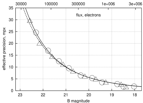
Figure 4: Effective precision of a single measurement $\bar{\sigma}$ (mean for $x$ and $y$ axes) for 2000 (circles) and 2002-2003 (triangles) epochs as a function of $B$. Centroiding error $\bar{\varepsilon}$ at average seeing and background noise is shown by solid (first epoch) and dashed (second epoch) lines. A scale is 1 mpx=100 $\mu$as.

The variance $\sigma_{im}^{2}$ of the noise ${\mathcal{N}}_{im}$ is the effective variance of a single measurement. Obviously, $\sigma_{im}^{2}\geq\varepsilon_{im}^{2}+\sigma_{\rm{at}}^{2}$. The size of $\sigma_{im}$ depends on the stellar magnitude $I_{i}$, the seeing $\theta_{im}$, the sky level $b_{m}$, the reduction parameters $k$ and $R$, etc. In the following, the analysis simplifies by using the improved expression for $\varepsilon_{im}$ that, as compared to Eq. (2), more adequately takes into account variations of $\theta_{im}$ and $b_{m}$, amounting to about $\pm 30$%, and is valid in a wide (about 5 mag) range of stellar brightness. Considering asymptotic dependences of $\varepsilon$ on $\theta$ and $b$ given by Irwin (Irwin (1985)) for bright and faint images, we modified Eq. (2) to

$$\varepsilon_{im}=\frac{\theta_{im}}{2.46\sqrt{I_{i}}}\left(1+\alpha_{0}I_{i}^{-0.7}\frac{\theta_{im}}{\theta_{0}}\sqrt{b_{m}/b_{0}}\right).$$ (25)

The second component in parentheses is significant for faint $B>21.5$ stars only. The $\theta_{im}$, or FWHM value, is available as a PSF model parameter (Sect.2). We have found that the variance of the normalized deviations $u_{im}/\varepsilon_{im}$ based on our new relation is almost independent from observation conditions. For that reason, the actual observed value of $\sigma_{im}^{2}$ was obtained as a systematic correction to $\varepsilon_{im}^{2}$:

$$\sigma_{im}^{2}=\varepsilon^{2}_{im}\left\langle\frac{1}{n_{l}-2}\sum\limits_{m}u_{lm}^{2}/\varepsilon_{lm}^{2}\right\rangle$$ (26)

where an average was taken over stars of approximately the same magnitude. Further averaging of $\sigma_{im}^{2}$ with respect to $i$ and $m$ (over observations) yielded the effective variance of a single measurement $\bar{\sigma}^{2}$ at average observational conditions during the considered epoch. Fig.4 presents both $\bar{\sigma}$ and the mean centroiding error $\bar{\varepsilon}$ corresponding to average observing conditions as a function of $B$. Because $\bar{\sigma}$ matches well the errors $\bar{\varepsilon}$ predicted by our numerical simulation, we conclude that the sum of all errors arising from different sources, including $\sigma_{\rm{at}}$, is small in comparison to $\varepsilon$, so that, approximately, $\bar{\sigma}\approx\bar{\varepsilon}$. This means that the astrometric precision depends only on errors of the photocentre determination which are random Gaussian and uncorrelated with time due their nature of arising from photon statistics. The latter property is very important since it forms the basis for substantial statistical improvements of the astrometric accuracy $\Delta(n_{i})$ for a sequence of $n_{i}$ frames with the increase of the number of measurements as

$$\begin{array}[]{lr}\Delta(n_{i})=\bar{\varepsilon}/\sqrt{n_{i}};&n_{i}\leq n_{\rm max}\\ \end{array}$$ (27)

where $\bar{\varepsilon}$ is the photocenter error at average observation condition. The estimate (27) is approximate since assumes the best situation with a diagonal covariance matrix of the system (23). The validity of Eq. (27) is limited with respect to the maximum amount of frames $n_{\rm max}$, at which the value of $\Delta(n_{i})$ reaches a floor set by systematic errors.

5 Testing the VLT temporal astrometric stability

5.1 The Allan variance

The simplest empiric validation of Eq. (27) and illustration of how this law works at different $n_{i}$, is associated with use of Allan variance $\sigma^{2}_{\rm Al}$ of the residuals $u_{im}$. This quantity (Pravdo & Shaklan Pravdo96 (1996)) is a function of time lag $\tau\leq n_{i}/2$ expressed in frames

$$\sigma^{2}_{\rm Al}(\tau)=\frac{1}{2(n_{i}+1-2\tau)}\sum\limits_{p=1}^{n_{i}+1-2\tau}\left[\tau^{-1}\sum\limits_{q=0}^{\tau-1}(u_{p+q}-u_{p+q+\tau})\right]^{2}$$ (28)

$\sigma^{2}_{\rm Al}(\tau)$ is a precision of the average of $u_{im}$ taken over $\tau$ frames, and so corresponds to $\Delta^{2}(\tau)$. For uncorrelated sets of $u_{im}$, the expected dependence $\sigma^{2}_{\rm Al}\sim\tau^{-1}$ is consistent with Eq. (27). In effort to increase the range of time lags, we performed computations of $\sigma^{2}_{\rm Al}$ treating all epoch frames as a single series of $n_{i}$ length. For miscellaneous reasons, $n_{i}$ varied from about $0.4M$ to $1.0M$. Results for stars of different $B$ magnitude classes are shown in Fig.5 (two bottom graphs). Though, in general, plots for separate stars follow the expected law $\tau^{-1}$ (straight lines with an ordinate $\bar{\varepsilon}^{2}$ at $\tau=1$), it is difficult to make any conclusion at $\tau\geq 10$. To smooth statistical fluctuations and exclude the dependence on the star brightness, we normalized individual $\sigma^{2}_{\rm Al}$ by $\bar{\varepsilon}^{2}$ (upper plot of Fig.5) and then performed averaging of results over all 169 stars. Obtained smooth functions $\langle\sigma^{2}_{\rm Al}/\bar{\varepsilon}^{2}\rangle$ (black dots) indicate no evidence of large systematic error, and extend a validity of the approximation $\sigma^{2}_{\rm Al}\sim\tau^{-1}$ at least to $\tau\approx 15$. Hence Eq.(27) is valid to about $n_{\rm max}\approx 15$. The asymptotic floor of the Allan variance at large $\tau$ is under the detection limit of this approach. We can claim however that with 15 frames, the resulting precision of the average is about 50$\mu$as for bright stars. In Sect.5.3, we renew this discussion to derive more exact estimate of $n_{\rm max}$.

Figure 5: Allan variance as a function of time lag $\tau$ for individual stars (dashed lines) in comparison to the $\tau^{-1}$ law (straight lines) in narrow magnitude ranges (two lower graphs) and the normalized variance $\sigma^{2}_{\rm Al}/\bar{\varepsilon}^{2}$ for all stars (upper plot). The average $\langle\sigma^{2}_{\rm Al}/\bar{\varepsilon}^{2}\rangle$ taken over all stars is shown by black dots. The plots refer to $x$ coordinate and 2000 epoch frames.

5.2 Distribution of residuals

The null hypothesis $H_{0}$ formally arising from above analysis is that the ${\mathcal{N}}_{im}$ component in Eqs. (23) represents an uncorrelated Gaussian noise. The ensuing consequences of this assumption are

• the averaging law, Eq. (27), and

• the absence of other noise components, including instrumental errors, with a noticable magnitude.

Figure 6: Histograms of individual normalized residuals ${u^{\prime}}_{im}$ in $x$ (a) and in $y$ ( b) for actual (steps) and simulated (smooth lines) observations, on 2000 (solid) and 2002 epochs (dashed lines); the same for normalized night average residuals $\bar{u}_{ip}/\sigma_{p}$ (c and d). Plots are drawn for bright $B<20.5$ stars.

We applied several statistical tests of our hypothesis. In the first test, we formed a histogrammic distribution $W$ of normalized deviations ${u^{\prime}}_{im}=\sqrt{n_{i}/(n_{i}-2)}{u}_{im}/\sigma_{im}$ and compared it with the distribution $W_{0}$ of these residuals expected when the data fulfill the hypothesis $H_{0}$. In order to obtain $W_{0}$, we performed some numerical simulations of observations with a typical spacing of frames on hour angles, and adding a Gaussian noise with a unit variance in $x$ and $y$ to the right side of Eqs. (23). Observed distributions $W$ were computed using all combinations of data sets available (2000 and 2003/2003 epoch frames, $x$ and $y$ data, with faint, bright, or a whole sample of stars). Fig.6a, b present an example of such a histogram $W$ for bright stars. Corresponding simulated distributions $W_{0}$ are shown by smooth curves, for which the same binning as for the computation of $W$ has been applied. Unlike ${\mathcal{N}}_{im}$, the distributions $W_{0}$ and $W$ are not Gaussians and have a more strongly peaked shape. The consistency of observed and model distributions by visual inspection is rather good. Numerically, it was estimated by $\chi^{2}$ values computed from differences between $W$ and $W_{0}$ in fixed binned intervals containing at least 5–10 data points. The $\chi^{2}$ values with corresponding degrees of freedom (Dof) are listed in Table 3 for faint, bright, or all stars, respectively. The $\chi^{2}$-test based on these data does not reveal a deviation of $W$ from $W_{0}$ at significance levels below 20%, which does not allow to reject our hypothesis $H_{0}$. Due to a limited number of data points, this test is however only sensitive to a central $\pm 2\sigma$ region of the distribution.

Table 3: $\chi^{2}$ values and Dof characterizing differences between $W$ and $W_{0}$

	faint	bright	all stars
	2000 epoch
$\chi^{2}$, $x$/$y$	20.1 /21.5	23.0/22.7	24.4/28.6
Dof	22	22	24
	2002/2003 epoch
$\chi^{2}$, $x$/$y$	20.8/11.6	25.5/17.2	27.8/27.1
Dof	18	20	22

Figure 7: The diffences $D_{n}$ between the observed and model cumulative frequency distributions of normalized residuals ${u^{\prime}}_{im}$ for 2000 epoch measurements in $y$ (bright stars)

We applied the more powerful Kolmogorov-Smirnov test to detect a potential difference between the observed and simulated distributions. For this purpose, we computed cumulative frequency distributions of observed and model normalized residuals ${u^{\prime}}_{im}$, and then obtained the difference $D_{n}$ between two distributions. A case with largest deviations for 2000 epoch measurements in $y$ with 1721 data points (bright stars only) is shown in Fig.7 where the differences $D_{n}$ are plotted as a function of the normalized deviation. The Kolmogorov-Smirnov test based on this plot (in this worst case max$|D_{n}|=0.024$) shows no significant difference between the model and measured distributions at 20% confidence level. Both tests applied thus do not reject hypothesis $H_{0}$ of a really normal distribution of ${\mathcal{N}}_{im}$ at approximately the same significance levels.

For another test, we considered nightly averages $\bar{u}_{ip}={\sum\limits_{m\in p}}u_{im}\sigma_{im}^{-2}/{\sum\limits_{m\in p}}\sigma_{im}^{-2}$, involving all observations of the $i$-th star within a single $p$-th night. Fig.6 c, d show observed and model frequency distribution of normalized residuals $\bar{u}_{ip}/\sigma_{p}$, where $\sigma_{p}$ is the error of the determination of $\bar{u}_{ip}$. A good agreement of the histograms of the observed statistics (both for bright and faint stars) with their expectations from model simulations, a symmetry, and the absence of large deviations (normally less than 1% of $\bar{u}_{ip}/\sigma_{p}$ values deviate at about 3 units) demonstrate excellent stability of the VLT instrumental system during time spans of a few nights. Compatability of the observed and model distributions is also confimed by the Kolmogorov-Smirnov- and $\chi^{2}$-tests.

5.3 Integral statistics

Table 4: Integral statistics $S_{0}$ and $S_{A}$ for bright $B<20.5$, faint $B>20.5$ stars, and for simulated observations

	$S_{0}^{x}$	$S_{0}^{y}$	error	$S_{A}^{x}$	$S_{A}^{y}$	error
	2000 epoch
model	0.997	0.985	-	0.749	0.839	-
bright	0.992	0.989	$\pm$0.021	0.784	0.849	$\pm$0.064
faint	0.982	0.988	$\pm$0.019	0.761	0.787	$\pm$0.054
	2002-2003 epoch
model	0.994	0.973	-	0.738	0.845	-
bright	0.973	0.961	$\pm$0.029	0.722	0.872	$\pm$0.067
faint	0.989	0.952	$\pm$0.026	0.744	0.874	$\pm$0.055

We also considered integral statistics $S_{0}^{2}=\langle\frac{1}{n_{i}-4}{\sum\limits_{m}}\frac{({u}_{im}-\bar{u}_{ip})^{2}}{\sigma_{im}^{2}}\rangle$, where averages are taken over all stars and nights, and $S_{A}^{2}=\langle\frac{1}{4}{\sum\limits_{p}}\bar{u}_{ip}^{2}/\sigma_{p}^{2}\rangle$, where an average is taken over all stars. These two statistics are either sensitive to the variation of systematic errors within a given night ($S_{0}$) or from one night to another ($S_{A}$), and therefore are a powerful indicator of their presence. The quantities $S_{0}$ and $S_{A}$, calculated separately for both coordinates $x$ and $y$, are listed in Table 4 for each epoch of observations together with the respective expected values $S_{0}(\rm mod)$ and $S_{A}(\rm mod)$, obtained from numerical simulations where random Gaussian noise ${\mathcal{N}}_{im}$ has been assumed. Errors due to a limited number of measurements indicate an 80% confidence interval for possible deviations of observed values from our model assumption. Observed statistics match well the model within the error limits.

The fact that we do not find an excess in the measured $S_{0}$ and $S_{A}$ values means that no or very small extra noise except ${\mathcal{N}}_{im}$ could be present in measurements. It is useful to estimate its upper limit. Suppose that the observed positions, besides of ${\mathcal{N}}_{im}$, are affected by some small systematic error that is constant within a night but varies between nights with an amplitude peculiar to a certain star. The observed value of $S_{A}^{2}(\rm obs)$ then exceeds its model expectation $S_{A}^{2}(\rm mod)$ by a small amount $S_{\rm sys}^{2}$ which is the average signal variance for a given star sample. These quantities are related by $S_{A}^{2}(\rm obs)=(\chi^{2}_{\rm Dof}/{\rm Dof})S_{A}^{2}(\rm mod)+S_{\rm sys}^{2}$. For statistical reasons, it is probable that the sampled value $S_{A}^{2}(\rm obs)$ is equal or below of its mathematical expectation $S_{A}^{2}(\rm mod)+S_{\rm sys}^{2}$. The largest value of $S_{\rm sys}^{2}$, according to Table 4, can exist in the $x$-axis measurements of bright stars (2000 epoch), for which we found $S_{\rm sys}^{2}/S_{A}^{2}(\rm mod)\leq 0.19$ at 20% confidence level. This is a ratio of a systematic to random error component for a single night series represented, in average, by 8 frames. In other words, the bias related to systematic errors is equal to a random component expected in positions averaged over $8/0.19=40$ frames. This is an estimate of $n_{\rm max}$ introduced in Eq.(27), more precise, as compared to that obtained in Sect.5.1. For $y$-coordinate, we obtain $n_{\rm max}=65$. Frames of 2002 yield $n_{\rm max}=120$ and 50 for the $x$ and $y$ axes correspondingly. With $n_{\rm max}=50$ adopted as a reliable limit, precision of a night series is about 30 $\mu$as.

5.4 Correlations

A final important test was carried out to investigate correlations in ${\mathcal{N}}_{im}$ which can negatively affect the averaging law (27). For that purpose, we computed the autocorrelation function of normalized residuals

$${r}(\tau)=H(\tau)\langle(u_{im_{1}}/\sigma_{im_{1}})(u_{im_{2}}/{\sigma_{im_{2}}})\rangle$$ (29)

of the argument $\tau=m_{2}-m_{1}$, which is equal to the difference of frame indexes and used as a time lag. Here, $H(\tau)=1-\tau/M$ is the weight function that compensates the increase of statistical variations at large $\tau$. Averaging is performed over the images of all stars. A corresponding computation of the expected correlation function $\hat{r}(\tau)$ was carried out with the model observations containing white noise with a unit variance. The observed ${r}(\tau)$ values computed for both coordinates $x$ and $y$ for bright $B<20.5$ mag stars are shown in Fig.8 along with the model function $\hat{r}(\tau)$ (mean for $x$ and $y$) and 1-$\sigma$ limits for statistical scatter of individual deviations. Oscillations in $\hat{r}(\tau)$ plot inherit a compound four-night structure of the series. Observed data in general follow the expected dependence, though with few isolated deviations over 2 sigma.

Figure 8: Observed autocorrelation function in $x$ (circles) and in $y$ (squares) as compared to the model function (solid line) with a 1-$\sigma$ tolerance limits (two dotted lines) and approximation (30) (dashed line)

Both $r$ and $\hat{r}$ are not identically zero as it could be expected for uncorrelated measurements. The observed systematic negative bias of correlations, however, is not due to instrumental errors but has a theoretical background (Lazorenko Lazorenko97 (1997)). In order to see this, consider Eqs. (23) for the $i$-th star. When the number of frames $M$ is large and the distribution of frames with hour angle is sufficiently random, all parameters in the system given by Eq. (23) become uncorrelated. Then $\xi_{i}^{x}$ is approximately equal to the average of $(\lambda_{im}^{x}-h_{im}^{x}+h_{i0}^{x}+{\mathcal{N}}_{im})$ taken with respect to the index $m$. In this approximation, one finds $u_{im}^{x}=(\lambda_{im}^{x}-h_{im}^{x}+h_{i0}^{x}+{\mathcal{N}}_{im})-\xi_{i}^{x}$. The term given in parentheses formally represents a solid time series of the ”time” argument $m$ with $m=1\ldots M$ measurements containing noise. With this approach, the $u_{im}^{x}$ values are the remainders of a time series after subtraction of the fitting polynomial (namely a constant $\xi_{i}^{x}$ in our case). The bias of the autocorrelation function shape due to subtraction of the best-fitting polynomial for measurements limited in time was also previously studied by Lazorenko (Lazorenko97 (1997)). The autocorrelation function $r^{\prime}$ of series remainders takes a particularly simple form if the power spectrum of measurement errors resembles a white noise (which is the case) with a unit variance and constant rate of data sampling. In this case, one obtains (Bakhonski et al. Bakhonski (1997))

$$r^{\prime}(\tau)=-\frac{2\varsigma}{M}\mbox{sinc}(2\pi\varsigma\tau/M)$$ (30)

where $\varsigma=0.56$, if the subtracted polynomial is presented by a constant, and $\mbox{sinc}(z)=\sin(z)/z$. One can see that $r^{\prime}\approx 0$ for large $M$ only (long series) while for small $M$ (limited number of sampled data) its value is absolutely large and negative. Due to simplification of our considerations, the measured and model functions are not exactly fitted by $r^{\prime}$, but good enough however to explain the statistical origin of the observed negative bias (Fig. 8). We conclude that no correlation is present in ${\mathcal{N}}_{im}$ at scales of several frames.

Table 5: Observed $\bar{r}$ and model $\bar{r}_{\rm{mod}}$ normalized correlations.

$\tau^{\prime}$	$\bar{r}^{x}$	$\bar{r}^{x}_{\rm{mod}}$	$\bar{r}^{y}$	$\bar{r}^{y}_{\rm{mod}}$	1-sigma error
	2000 epoch
1	-0.17	-0.18	-0.22	-0.24	$\pm 0.05$
2	-0.17	-0.10	-0.20	-0.24	$\pm 0.07$
3	-0.42	-0.38	-0.25	-0.23	$\pm 0.09$
	2002-2003 epoch
1	-0.15	-0.14	-0.26	-0.25	$\pm 0.06$
2	-0.19	-0.20	-0.32	-0.23	$\pm 0.07$
3	-0.35	-0.26	-0.13	-0.19	$\pm 0.10$

Correlation at time scales of few days were studied using normalized nightly-average residuals $\bar{u}_{ip}/\sigma_{p}$. We computed correlations

$$\bar{r}(\tau^{\prime})=\langle(\bar{u}_{ip_{1}}/\sigma_{p_{1}})(\bar{u}_{ip_{2}}/\sigma_{p_{2}})\rangle$$ (31)

as a function of the time lag $\tau^{\prime}=p_{2}-p_{1}$ between two nights with indexes $p_{1}$ and $p_{2}$, expressed in days. The values of $\bar{r}$ for the observed data and corresponding model value $\bar{r}_{\rm{mod}}$ are given in Table 5. Apparently, there is a strong negative bias in $\bar{r}$ due to a very limited number of data points in our 4-night series. This bias, however, is well-modelled using uncorrelated noise ${\mathcal{N}}_{im}$, which confirms previous conclusions that there are no traces of instrumental signature in VLT observations at time scales of few nights, and supports the validity of the averaging law (27).

5.5 Two-year stability

Figure 9: Difference in the chromatic parameters $\rho_{i}$ and $d_{i}$ between the two epochs, normalized by the error of this difference computation (dots). Ellipses are drawn at 1% (dashed line) and 5% (solid) significance level. A straight line shows the direction of point displacements due to the actual change of star colours.

Given only two epoch measurements, no conclusions on a long-term astrometric stability of the VLT can be made based on positional information. Considering extreme importance of this problem, we present here indirect analysis of this issue based, instead of positions, on a comparison of chromatic $\rho_{i}$ and $d_{i}$ parameters computed from independent runs of 2000 and 2002/2003 epochs. If one assumes constant colours for the observed stars, these parameters should coincide within error bars. A change of the VLT characteristics, depending on stellar colours, should result in an additional difference. Fig.9 shows normalized differences between $\rho_{i}$ and $d_{i}$ between the two epochs, where ellipses refer to significance levels of 1% or 5%, respectively. Some points represent outliers, testifying the presence of systematic errors. The largest residuals for bright stars in the right bottom however occur along a line $\rho_{i}=-1.2d_{i}$ that is peculiar to the distribution of chromatic parameters shown in Fig. 3. It is therefore very likely that these deviations are caused by a change in stellar colour. Some other large deviations appear to be related to stars in outer regions of the observed field where the method seems to give biased results. Except for these outliers, the distribution of points in Fig. 9 resembles a Gaussian, which is an indicator of a rather good astrometric stability of the VLT even at very long time scales. It should be stressed that above test is insensitive to non-chromatic type of errors and therefore is only indicative.

6 Conclusion

Our results reveal an exceptionally good astrometric performance of the VLT and its camera FORS1. Thus, the precision $\bar{\varepsilon}$ of the position of a bright star reaches 200 $\mu$as for a single measurement, which fairly well corresponds to the former 300 $\mu$as estimate obtained for FORS2 camera (Paper I). Both cameras thus give similarly good results. The term ”bright star” refers to unsaturated images containing 1–3$\cdot 10^{6}$ electrons and may correspond to different stellar magnitudes depending on the exposure, filter, and seeing. Most importantly, we found negligibly small systematic errors of instrumental and other origin. In fact, no traces of these ’dangerous’ errors were found at time intervals up to 4 days. Due to this fact, the precision for a frame series improves as $\bar{\varepsilon}/\sqrt{n_{i}}$, and at ${n_{i}}=50$ reaches 30 $\mu$as for FORS1 and 40 $\mu$as for FORS2. With use of FORS2, the observation time needed to obtain this accuracy is about 1 hour if short 15 s exposures and a $2\times 2$ binning of pixel reading is used. We conclude that the VLT with cameras FORS1/2, due to its enormous collecting light power, fine optical performance, and effective averaging of wave-front distortions over a large aperture, is a powerful instrument that can be used efficiently for high-precision astrometric observations of short-term events, in particular, of planetary microlensing.

- (1) Avila, G., Rupprecht, G. & Beckers, J. M. 1997, Proc. SPIE 2871, 1135
- (2) Bakhonski, A.V., Kostjutshenko, V.L., & Lazorenko, P.F. 1997, Kinematics and Phys. Celest. Bodies 13, 5, 50
- (3) Beaulieu, J.-P., Bennett, D.P., Fouque, P., et al. 2006, Nature, 439, 437
- (4) Boden, A.F., Shao, M., & Van Buren, D. 1998, ApJ 502, 538
- (5) Bond, J.A., Udalski, A., Jaroszynski, M. et al. 2004, ApJ 606, L155
- (6) Colavita, M.M., Boden, A.F., & Crawford, S.L. 1998, Proc. SPIE 3350, 776
- (7) Dominik, M. 1999, A&A 349, 108
- (8) Dominik, M., & Sahu, K.C. 2000, ApJ 534, 231
- (9) Irwin, M.J. 1985, MNRAS, 214, 575
- (10) Jaroszyński, M., & Paczyński, B. 2002, Acta Astron. 52, 361
- (11) Gaudi, B.S., & Gould, A. 1997, ApJ 486, 85
- (12) Gaudi, B.S. 1998, ApJ 506, 533
- (13) Gaudi, B.S., & Han. C. 2004, ApJ 611, 528
- (14) Gould, A., Udalski, A., Bennett, D., et al. 2006, ApJ 644, L37
- (15) Han, C., & Chunguk, L. 2002, MNRAS, 329, 163
- (16) Hardy, S.J., & Walker, M.A. 1995, MNRAS 276, L79
- (17) Høg, E., Novikov, I.D., & Polnarev, A.G. 1995, A&A 294, 287
- (18) Lane, B.F., & Muterspagh, M.W. 2004, ApJ, 601, 1129
- (19) Lazorenko, P.F. 1997, Kinematics and Phys. Celest. Bodies 13, 2, 63
- (20) Lazorenko, P.F., & Lazorenko, G.A. 2004, A&A 427, 1127
- (21) Lazorenko, P.F. 2006, A&A 449, 1271
- (22) Lindegren, L. 1980, A&A 89, 41
- (23) Miyamoto, M., & Yoshii, Y. 1995, AJ 110, 1427
- (24) Monet, D.G., Dahn, C.C., Vrba, F.J., et al. 1992, AJ, 103, 638
- (25) Motch, C., Zavlin, V.E., & Haberl, F. 2003, A&A, 408, 323
- (26) Paczyński, B. 1998, ApJ, 494, L23
- (27) Pravdo, S., & Shaklan, S. 1996, AJ 465, 264
- (28) Pravdo, S.H, Shaklan, S.B., Lloyd, J. et al. 2005, ASP Conf. Series, 338, 288
- (29) Pravdo, S.H, Shaklan, S.B., Wiktorowicz, S.J. et al. 2006, ApJ, 649, 389
- (30) Quirrenbach, A., Henning, T., & Queloz, D., 2004, Proc. SPIE 5491, 424
- (31) Safizadeh, N., Dalal, N., & Griest, K. 1999, ApJ, 522, 512
- (32) Udalski, A., Jaroszynski, M., Paczyński, B., et al. 2005, ApJ, 628, L109
- (33) Wittkowski, M., Ballester, P., Canavan, T. et al. 2004, Proc. SPIE 5491, 617