Abstract

We determine from Polyakov loop correlators the screening masses in the deconfined phase of the (3+1)$d$ SU(3) pure gauge theory at finite temperature near the transition, for two different channels of angular momentum and parity. Their ratio is compared with that of the massive excitations with the same quantum numbers in the 3$d$ 3-state Potts model in the broken phase near the transition point at zero magnetic field. Moreover we study the inverse decay length of the correlation between the real parts and between the imaginary parts of the Polyakov loop and compare the results with expectations from perturbation theory and mean-field Polyakov loop models.

  ^∗ e-mail addresses: rfalcone,fiore,gravina,papa@cs.infn.it

1 Introduction

The essential features of confinement, of the deconfinement phase transition at finite temperature and of the deconfined phase in QCD can be studied without loss of relevant dynamics in the regime of infinitely massive quarks or, equivalently, in the SU(3) pure gauge theory.

The (3+1)$d$ SU(3) pure gauge theory at finite temperature undergoes a confinement/deconfinement phase transition associated with the breaking of the center of the gauge group, Z(3) [1, 2]. This transition is weakly first order [3, 4, 5, 6, 7] and the order parameter is the Polyakov loop [1, 2].

In general, the deconfinement transition in the $(d+1)$-dimensional SU(N) pure gauge theory at finite temperature can be put in relation with the order/disorder [8] phase transition of the $d$-dimensional Z(N) spin model through the Svetitsky-Yaffe conjecture [9]. According to this conjecture, when the transition is second order the gauge theory and the spin model belong to the same universality class and therefore share critical indices, amplitude ratios and correlation functions at criticality. There are so many numerical evidences in favor of this conjecture – see, for instance, Refs. [10, 11, 12, 13, 14, 15, 16] and, for a review, Ref. [17] – that there is no residual doubt about its validity.

In the case of first order phase transitions, as for the (3+1)$d$ SU(3) pure gauge theory, the Svetitsky-Yaffe conjecture is not applicable in strict sense, since the correlation length keeps finite at the transition point and a universal behavior, independent of the details of the microscopic interactions, cannot be established. Therefore there are no a priori reasons why the critical dynamics of (3+1)$d$ SU(3) and of its would-be counterpart spin model, 3$d$ Z(3) or 3-state Potts model [18, 19], should look similar. It turns out, however, that for both these theories the phase transition is weakly first order, which means that the correlation length at the transition point, although finite, becomes much larger than the lattice spacing. This leads to the expectation that the two theories may have some long distance aspects in common and that some specific issues of SU(3) in the transition region can be studied taking the 3$d$ 3-state Potts model as an effective model.

Since there are no critical indices to compare, a test of this possibility could be based on the comparison of the spectrum of massive excitations of the 3$d$ 3-state Potts model in the broken phase near the transition at zero magnetic field with the spectrum of the inverse decay lengths of Polyakov loop correlators in the (3+1)$d$ SU(3) gauge theory in the deconfined phase near the transition. If universality would apply in strict sense, these spectra should exhibit the same pattern, as suggested by several numerical determinations in the 3$d$ Ising class [20, 21, 22, 23].

In this paper we determine the low-lying masses of the spectrum of the (3+1)$d$ SU(3) pure gauge theory at finite temperature in the deconfined phase near the transition in two different sectors of parity and orbital angular momentum, 0⁺ and 2⁺, and compare their ratio with that of the corresponding massive excitations in the phase of broken Z(3) symmetry of the 3$d$ 3-state Potts model, determined in Ref. [24].

In fact, we extend our numerical analysis to temperatures far away from the transition temperature $T_{t}$ in order to look for possible “scaling” of the fundamental masses with temperature. Moreover, we consider also the screening masses resulting from correlators of the real parts and of the imaginary parts of the Polyakov loop. These determinations can represent useful benchmarks for effective models of the high-temperature phase of SU(3), such as those based on mean-field theories of the Polyakov loop, suggested by R. Pisarski [25].

The paper is organized as follows: in Section 2 we describe the methods used to extract the screening masses through Polyakov loop correlators in (3+1)$d$ SU(3); in Section 3 we present our numerical results and compare them with expectations from the 3$d$ 3-state Potts model and from Polyakov loop effective models; in the last Section we draw our conclusions.

2 Screening masses from Polyakov loop correlators

In this Section we define the general procedure for extracting screening masses in (3+1)$d$ SU(3) at finite temperature from correlators of the Polyakov loop,

$$P(x,y,z)=\mbox{Tr}\prod_{n_{t}=1}^{N_{t}}U_{4}(x,y,z,n_{t}a)\ ,$$ (1)

where $N_{t}$ is the number of lattice sizes in the temporal direction and $a$ is the lattice spacing.

The point-point connected correlation function is defined as

$$\Gamma_{i_{0}}(r)=\langle P_{i}^{\dagger}P_{i_{0}}\rangle-\langle P_{i}^{\dagger}\rangle\langle P_{i_{0}}\rangle\ ,$$ (2)

where $i$ and $i_{0}$ are the indices of sites and $r$ is the distance between them. The large-$r$ behavior of the point-point connected correlation function is determined by the correlation length of the theory, $\xi_{0}$, or, equivalently, by its inverse, the fundamental mass. In order to extract the fundamental mass it is convenient to define the wall-wall connected correlation function, since numerical data in this case can be directly compared with exponentials in $r$, without any power prefactor.

The 0⁺-channel connected wall-wall correlator in the $z$-direction is defined as

$$G(|z_{1}-z_{2}|)=\mbox{Re}\langle\bar{P}(z_{1})\bar{P}(z_{2})^{\dagger}\rangle-|\langle P\rangle|^{2}\ ,$$ (3)

where

$$\bar{P}(z)=\frac{1}{N_{x}N_{y}}\sum_{n_{x}=1}^{N_{x}}\sum_{n_{y}=1}^{N_{y}}P(n_{x}a,n_{y}a,z)\ ,$$ (4)

represents the Polyakov loop averaged over the $xy$-plane at a given $z$. Here and in the following, $N_{i}$ ($i=x,y,z$) is the number of lattice sites in the $i$-direction. The wall average implies the projection at zero momentum in the $xy$-plane.

The correlation function (3) takes contribution from all the screening masses in the 0⁺ channel. In fact, the general large distance behavior for the function $G(|z_{1}-z_{2}|)$, in an infinite lattice, is:

$$G(|z_{1}-z_{2}|)=\sum_{n}a_{n}e^{-m_{n}|z_{1}-z_{2}|}\ ,$$ (5)

where $m_{0}$ is the fundamental mass, while $m_{1}$, $m_{2}$, … are higher masses with the same angular momentum and parity (0⁺) quantum numbers of the fundamental mass. On a periodic lattice the above equation must be modified by the inclusion of the so called “echo” term:

$$G(|z_{1}-z_{2}|)=\sum_{n}a_{n}\biggl{[}e^{-m_{n}|z_{1}-z_{2}|}+e^{-m_{n}(N_{z}-|z_{1}-z_{2}|)}\biggr{]}\;.$$ (6)

The fundamental mass in a definite channel can be extracted from wall-wall correlators by looking for a plateau of the effective mass,

$$m_{\mbox{\footnotesize eff}}(z)=\ln\frac{G(z-1)}{G(z)}$$ (7)

at large distances. For the 2⁺-channel, we used the variational method [26, 27], which consists in defining several wall-averaged operators with 2⁺ quantum numbers and in building the matrix of cross-correlations between them. The eigenvalues of this matrix are single exponentials of the effective masses in the given channel. The variational method is usually adopted to determine massive excitations above the fundamental one in the given channel. In our case, however, it turned out that this method improved the determination of the fundamental mass in the 2⁺-channel, but did not lead to determine higher excitations. Our choice of wall-averaged operators in the 2⁺-channel is inspired by Ref. [28] and reads

$$\bar{P}_{n}(z)=\frac{1}{N_{x}N_{y}}\sum_{n_{x}=1}^{N_{x}}\sum_{n_{y}=1}^{N_{y}}P(n_{x}a,n_{y}a,z)\biggl{[}P(n_{x}a+na,n_{y}a,z)-P(n_{x}a,n_{y}a+na,z)\biggr{]}\ .$$ (8)

In most cases we have taken 8 operators, corresponding to different values of $n$, with the largest $n$ almost reaching the spatial lattice size $N_{x}$. We have determined the 0⁺ and the 2⁺ fundamental masses in lattice units, $\hat{m}_{0^{+}}$ and $\hat{m}_{2^{+}}$, over a wide interval of temperatures above the transition temperature $T_{t}$ of (3+1)$d$ SU(3) and have studied

- if in some region, lying strictly above $T_{t}$, a scaling law can be found for the fundamental correlation length $\hat{\xi}_{0}=1/\hat{m}_{0^{+}}$;

- if $\hat{m}_{2^{+}}$ has the same scaling behavior as $\hat{m}_{0^{+}}$;

- how the ratio $m_{2^{+}}/m_{0^{+}}$ compares with the ratio of the corresponding excitations in the broken phase of 3$d$ 3-state Potts model near the transition, $m_{2^{+}}/m_{0^{+}}=2.43(10)$, found in Ref. [24] on a 48³ lattice.

We consider also correlators of the (wall-averaged) real and imaginary parts of the Polyakov loop, defined as

$$G_{R}(|z_{1}-z_{2}|) = \langle\mbox{Re}\bar{P}(z_{1})\mbox{Re}\bar{P}(z_{2})\rangle-\langle\mbox{Re}\bar{P}(z_{1})\rangle\langle\mbox{Re}\bar{P}(z_{2})\rangle\;,$$ (9)

$$G_{I}(|z_{1}-z_{2}|) = \langle\mbox{Im}\bar{P}(z_{1})\mbox{Im}\bar{P}(z_{2})\rangle\;.$$ (10)

The corresponding screening masses, $\hat{m}_{R}$ and $\hat{m}_{I}$, can be extracted in the same way as for the 0⁺ mass.

We have studied the ratio $m_{I}/m_{R}$ over a wide interval of temperatures above the transition temperature $T_{t}$ of (3+1)$d$ SU(3) and seen how it compares with the prediction from high-temperature perturbation theory, according to which it should be equal to 3/2 [30, 31], and with the prediction from the mean-field Polyakov loop model of Ref. [29], according to which it should be equal to 3 in the transition region. The interplay between the two regimes should delimit the region where mean-field Polyakov loop models should be effective.

3 Numerical results

We used the Wilson lattice action and generated Monte Carlo configurations by a combination of the modified Metropolis algorithm [32] with over-relaxation on SU(2) subgroups [33]. The error analysis was performed by the jackknife method over bins at different blocking levels. We performed our simulations on a 16${}^{3}\times$4 lattice, for which $\beta_{t}=5.6908(2)$ [34], over an interval of $\beta$ values ranging from 5.69 to 9.0.

Screening masses are determined from the plateau of $m_{\mbox{\footnotesize eff}}(z)$ as a function of the wall separation $z$. In each case, the plateau mass is taken as the effective mass (with its error) belonging to the plateau and having the minimal uncertainty. We define plateau the largest set of consecutive data points, consistent with each other within 1$\sigma$. This procedure is more conservative than identifying the plateau mass and its error as the results of a fit with a constant on the effective masses $m_{\mbox{\footnotesize eff}}(z)$, for large enough $z$. To illustrate our definition of plateau mass, let us apply it to Figs. 3(b) and 4(a), which give respectively the $\hat{m}_{2^{+}}$ and the $\hat{m}_{I}$ effective masses at $\beta=5.74$ versus the separation $z$ between walls (the cases of $\hat{m}_{2^{+}}$ and $\hat{m}_{I}$ are usually the most problematic for the determination of the plateau mass). In Fig. 3(b), according to our definition, the plateau is formed by the points at $z=3$, 4 and 5, since they are compatible each other within 1$\sigma$; the plateau mass is taken as the effective mass at $z=3$, since this effective mass has the smallest uncertainty among the three masses belonging to the plateau. In Fig. 4(a), according to our definition, the plateau is formed by the points at $z=4$, 5 and 6, since they are compatible each other within 1$\sigma$; the plateau mass is taken as the effective mass at $z=4$, since this effective mass has the smallest uncertainty among the three masses belonging to the plateau.

Just above the critical value $\beta_{t}$ we find a large correlation length, which is not of physical relevance. It is instead a genuine finite size effect [8] related to tunneling between degenerate vacua. This effect disappears by going to larger lattice volumes or moving away from $\beta_{t}$ in the deconfined phase. Indeed, by increasing $\beta$ one can see that the symmetric phase becomes less and less important in the Monte Carlo ensemble, up to disappearance; then, for large enough $\beta$, also the structure with three-degenerate Z(3) sectors disappears, leaving only the real sector of Z(3). This is illustrated in Fig. 1 where the scatter plot of the Polyakov loop is shown for three representative $\beta$ values.

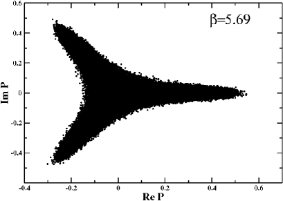
(a)

(b)

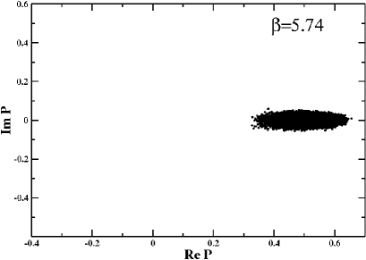
(c)

Figure 1: Scatter plots of the real and imaginary part of the Polyakov loop at (a) $\beta=5.69\simeq\beta_{t}$, (b) $\beta=5.71$ and (c) $\beta=5.74$.

Tunneling can occur between the symmetric and the broken phase, and between the three degenerate vacua of the deconfined phase. The former survives only in a short range of temperatures around $\beta_{t}$, and at $\beta\simeq 5.71$ has almost completely disappeared, as we can see from Fig 1(b). When tunneling is active, the correlation function has the following expression [8]:

$$G(|z_{1}-z_{2}|)\sim a_{0}e^{-m_{0}|z_{1}-z_{2}|}+b_{0}e^{-m_{t}|z_{1}-z_{2}|}\;,$$ (11)

where $m_{t}$ is the inverse of the tunneling correlation length and is generally much smaller than the fundamental mass $m_{0}$ and therefore behaves as a constant additive term in the correlation function. In (11) we have taken into account only the lowest masses in the spectrum and omitted the “echo” terms. The dependence on $m_{t}$ in the correlation function can be removed by extracting the effective mass by use of the combination

$$m_{\mbox{\footnotesize eff}}(z)=\ln\frac{G(z)-G(z+1)}{G(z+1)-G(z+2)}\ .$$ (12)

For $\beta\gtrsim 5.71$ the only active tunneling is among the three broken minima. However, the separation among them is so clear (see, for instance, Fig. 2(a)), that it is possible to “rotate” unambiguously all the configurations to the real sector (see Fig. 2(b)) and to treat them on the same ground.

We have performed simulations for several values of $\beta$ in the deconfined phase, up to $\beta=9.0$, with a statistics of a few hundred thousand “measurements” at each $\beta$ value. Simulations have been performed on the PC cluster “Majorana” of the INFN Group of Cosenza.

As discussed in the Introduction and in Section 2, our typical observable is a screening mass in a given channel of angular momentum and parity, identified as the plateau value in the plot of the effective mass as a function of the separation $z$ between two-dimensional walls. The procedure to determine the plateau value has been illustrated in Section 2. A typical example of the behavior of the effective mass with $z$ is shown in Fig. 3 for the 0⁺ and the 2⁺ channels and in Fig. 4 for the masses $\hat{m}_{I}$ and $\hat{m}_{R}$ extracted from Eqs. (9) and (10). The deviation from the plateau value at small $z$ can be attributed to lattice artifacts and to the possible effect of other states with excited masses in the same channel. Our determinations refer only to the fundamental masses in a given channel. The behavior with $\beta$ of the fundamental masses in the 0⁺ and the 2⁺ channels is given in Fig. 5. In Fig. 6 we show instead the masses $\hat{m}_{R}$ and $\hat{m}_{I}$ for varying $\beta$. A summary of all our results is presented in Table 1. We observe from Table 1 that $\hat{m}_{0^{+}}$ and $\hat{m}_{R}$ are consistent within statistical errors, this indicating that the Polyakov loop correlation is dominated by the correlation between the real parts. Our results for $\hat{m}_{0^{+}}$ at $\beta=5.70$ and $\beta=5.90$ ($T\simeq 3T_{t}/2$) can be compared with the corresponding determinations on a $4\times 8^{2}\times 16$ lattice of Ref. [35], which give 0.27${}^{+0.01}_{-0.02}$ and 0.64(1), respectively. The $\sim$15$\%$ disagreement can be taken as a measure of the systematic effects involved in the whole procedure for the determination of masses. We cannot make a direct comparison with the determination for $\hat{m}_{0^{+}}$ at $\beta=5.93$ on a 16${}^{3}\times 4$ lattice of Ref. [36], since we did not perform simulations at this value of $\beta$. We observe, however, that the determination of Ref. [36], which gives 0.73(5) according to our definition of plateau mass value, agrees with the results for the two adjacent $\beta$ values in our Table, $\beta=5.90$ and $\beta=9.0$.

We can see that the fundamental mass in the 0⁺ channel, as well as $\hat{m}_{R}$, becomes much smaller than 1 at $\beta_{t}$, as expected for a weakly first order phase transition. In the cases of $\hat{m}_{0^{+}}$ and of $\hat{m}_{R}$ we have made some determinations below $\beta_{t}$ (see Figs. 5 and 6). It turns out that masses in lattice units take their minimum value just at $\beta_{t}$, where there is a “cusp” in the $\beta$-dependence. Such a behaviour was observed also by the authors of Ref. [37], whose results, when the comparison is possible, agree with ours.

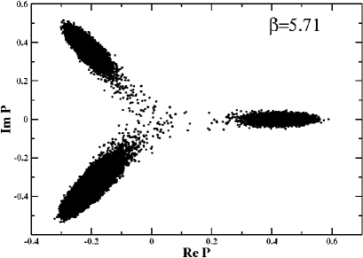
(a)

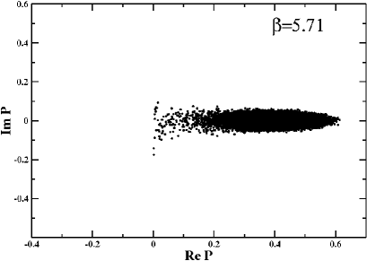
(b)

Figure 2: (a) Typical scatter plot of the complex order parameter $P$ for $\beta$ larger than 5.705 on a 16${}^{3}\times 4$ lattice. There are no states in the symmetric phase, but tunneling survives between the three broken minima.
(b) Same as (a) with the tunneling between broken minima removed by the “rotation” to the real phase.

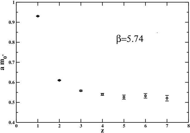
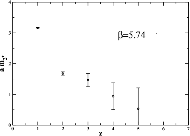
(a) (b)

Figure 3: Effective mass in the 0⁺ (a) and the 2⁺ (b) channel as a function of the separation between walls on the $(x,y)$ plane at $\beta=5.74$.

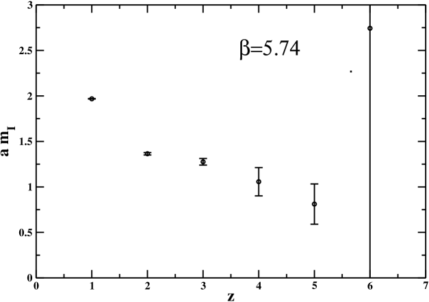
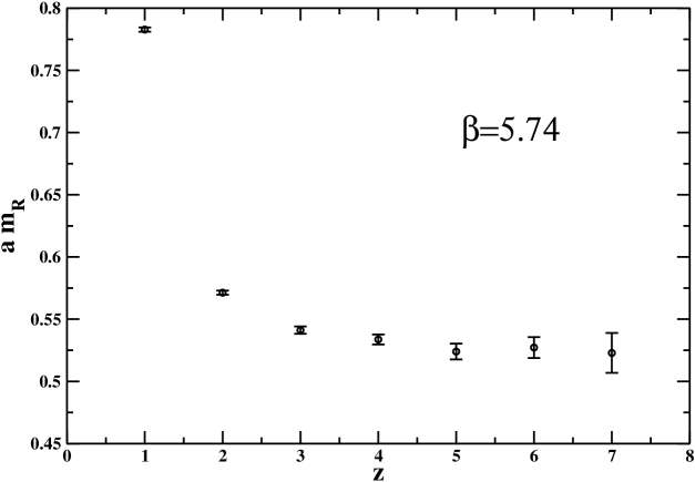
(a) (b)

Figure 4: Effective mass $\hat{m}_{I}$ (a) and $\hat{m}_{R}$ (b) as a function of the separation between walls on the $(x,y)$ plane at $\beta=5.74$.

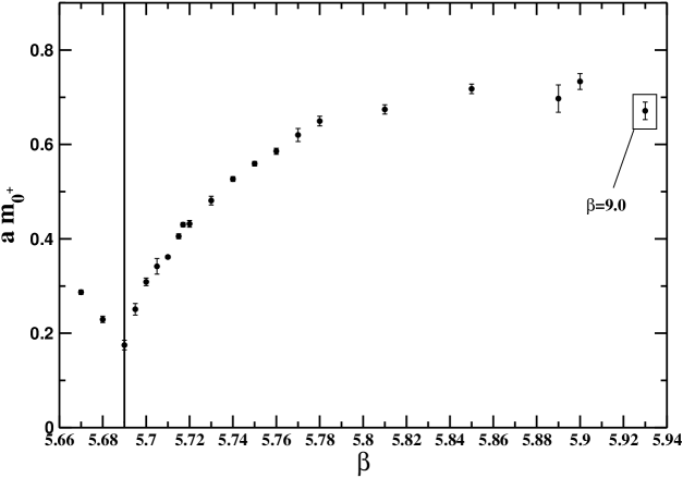
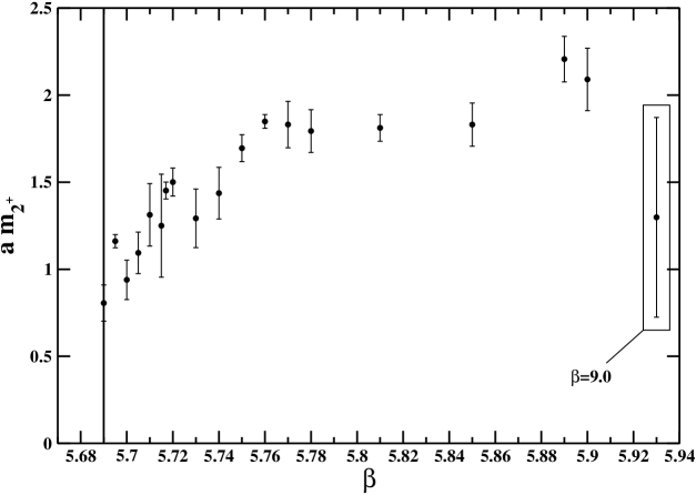
(a) (b)

Figure 5: Screening mass in the 0⁺ (a) and in the 2⁺ (b) channel as a function of $\beta$.

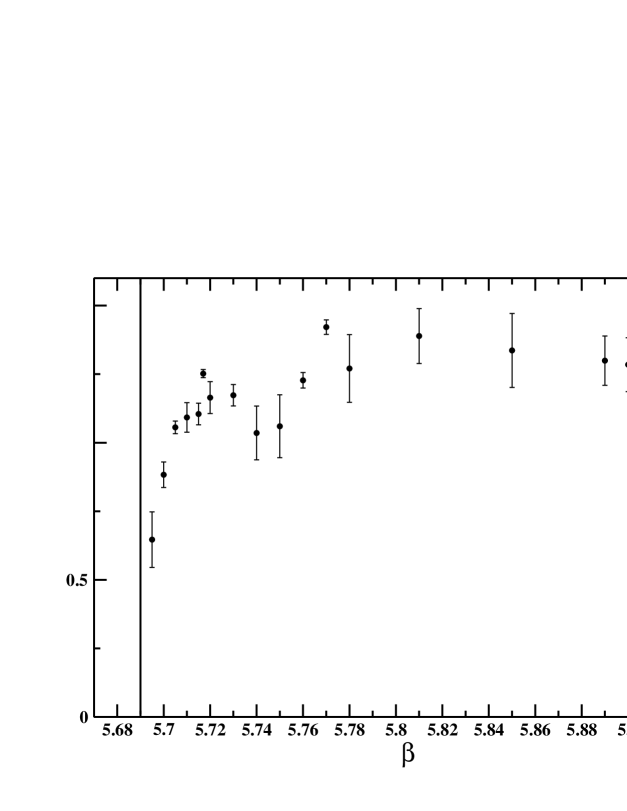
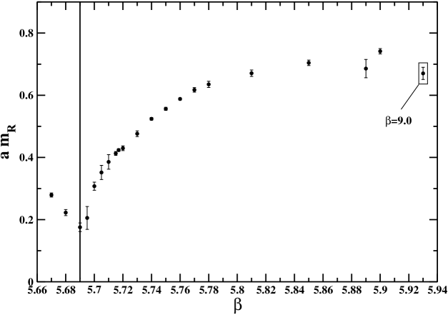
(a) (b)

Figure 6: Screening mass $\hat{m}_{I}$ (a) and $\hat{m}_{R}$ (b) as a function of $\beta$.

Table 1: Summary of the results for the fundamental masses in the $0^{+}$ and $2^{+}$ channels, for $\hat{m}_{I}$ and $\hat{m}_{R}$ and for some mass ratios.

$\beta$	$\hat{m}_{0^{+}}$	$\hat{m}_{2^{+}}$	$m_{2^{+}}$/$m_{0^{+}}$	$\hat{m}_{I}$	$\hat{m}_{R}$	$m_{I}/m_{R}$	stat.
5.67	0.2870(46)	-	-	-	0.2793(65)	-	750k
5.68	0.2293(67)	-	-	-	0.2226(97)	-	250k
5.69	0.175(10)	0.81(10)	4.61(86)	-	0.176(14)	-	770k
5.695	0.251(12)	1.161(38)	4.63(38)	0.65(10)	0.205(37)	3.07(87)	320k
5.70	0.3088(80)	0.94(11)	3.04(45)	0.883(47)	0.307(13)	2.87(27)	770k
5.705	0.342(17)	1.09(12)	3.20(50)	1.056(23)	0.352(23)	2.86(15)	750k
5.71	0.3615(30)	1.31(18)	3.63(53)	1.092(54)	0.386(23)	2.98(19)	770k
5.715	0.4054(51)	1.25(30)	3.08(77)	1.105(40)	0.4129(61)	2.68(14)	250k
5.717	0.4301(46)	1.452(49)	3.38(15)	1.252(15)	0.4237(43)	2.955(65)	320k
5.72	0.4319(69)	1.500(80)	3.47(24)	1.164(58)	0.4296(76)	2.71(18)	770k
5.73	0.4811(92)	1.29(17)	2.69(40)	1.173(39)	0.4762(92)	2.46(13)	170k
5.74	0.5267(52)	1.44(15)	2.73(31)	1.035(98)	0.5241(44)	1.98(20)	770k
5.75	0.5592(50)	1.695(77)	3.03(17)	1.06(11)	0.5562(49)	1.91(22)	770k
5.76	0.5857(65)	1.849(39)	3.16(10)	1.227(28)	0.5880(36)	2.087(61)	770k
5.77	0.620(14)	1.83(13)	2.95(28)	1.421(26)	0.6173(73)	2.303(70)	60k
5.78	0.650(10)	1.79(12)	2.76(23)	1.27(12)	0.635(10)	2.00(23)	60k
5.81	0.6742(99)	1.812(77)	2.69(15)	1.39(10)	0.671(10)	2.07(18)	190k
5.85	0.718(10)	1.83(12)	2.55(21)	1.34(13)	0.7042(87)	1.90(21)	110k
5.89	0.697(29)	2.21(13)	3.17(32)	1.299(90)	0.686(29)	1.89(21)	190k
5.90	0.734(17)	2.09(18)	2.85(31)	1.284(98)	0.7415(87)	1.73(15)	215k
9.0	0.671(19)	1.30(57)	1.93(91)	1.10(11)	0.670(19)	1.64(23)	200k

3.1 Scaling behavior and comparison with the Potts model

It would be interesting to find a scaling law for the fundamental mass in the $0^{+}$ channel, which looks like the one which holds for a second order phase transition, with a suitable critical exponent. There is, however, an important caveat: while the correlation length in lattice units diverges at a second order critical point, it keeps finite at a first order transition point. Therefore, any second-order-like scaling law, when applied to the region near a first order phase transition, should be taken as an effective description, which cannot hold too close to the transition point.

With this spirit, we have compared our data with the scaling law

$$\Bigg{(}\frac{\beta_{1}-\beta_{t}}{\beta_{2}-\beta_{t}}\Bigg{)}^{\nu}\sim\frac{\hat{m}_{0^{+}}(\beta_{1})}{\hat{m}_{0^{+}}(\beta_{2})}\ ,$$ (13)

where $\hat{m}_{0^{+}}(\beta_{1})$ and $\hat{m}_{0^{+}}(\beta_{2})$ are the fundamental masses in the $0^{+}$ channel at $\beta_{1}$ and $\beta_{2}$, respectively. This scaling law (13) is an approximation of the law

$$\Bigg{(}\frac{T_{1}-T_{t}}{T_{2}-T_{t}}\Bigg{)}^{\nu}\sim\frac{\hat{m}_{0^{+}}(T_{1})}{\hat{m}_{0^{+}}(T_{2})}\ ,$$ (14)

valid in an interval around $T_{t}$ short enough that the linear approximation $T_{1}-T_{t}\propto\beta_{1}-\beta_{t}$ holds. We have considered several choices of $\beta_{1}$ and found that for each of them there is a wide “window” of $\beta$ values above $\beta_{t}$ where the scaling law (13) works, with a “dynamical” exponent $\nu$. Our results are summarized in Table 2. For $\beta_{1}$=5.72 and 5.73, which lie well inside this “window”, the parameter $\nu$ is compatible with $\nu$=1/3, suggested in Ref. [38] to apply to the standard correlation function. For $\beta_{1}$=5.72 we have calculated also the $\chi^{2}$/d.o.f. when $\nu$ is put exactly equal to 1/3, getting $\chi^{2}$/d.o.f.=0.75 in the window from $\beta=5.715$ to $\beta=5.78$. In Fig. 7 we show, for this choice of $\beta_{1}$, the comparison between data and the “scaling” function with $\nu$ set equal to 1/3.

Table 2: Summary of the fits of the mass ratios ${\hat{m}_{0^{+}}(\beta_{1})}/{\hat{m}_{0^{+}}(\beta)}$ with the function $((\beta_{1}-\beta_{t})/(\beta-\beta_{t}))^{\nu}$. The second column contains the largest window of $\beta$ values for which the fit has a $\chi^{2}$/d.o.f. lower than 1.

$\beta_{1}$	window of $\beta$ values	$\nu$	$\chi^{2}$/d.o.f.
5.75	5.70 - 5.78	0.3619(90)	0.90
5.74	5.70 - 5.78	0.365(11)	0.92
5.73	5.695 - 5.85	0.329(12)	0.77
5.72	5.695 - 5.78	0.354(12)	0.73
5.717	5.715 - 5.81	0.3228(94)	0.69
5.715	5.695 - 5.78	0.358(10)	0.86
5.71	5.72 - 5.78	0.3951(76)	0.33
5.705	5.705 - 5.78	0.448(22)	0.89
5.70	5.695 - 5.90	0.3141(58)	0.94
5.695	5.695 - 5.90	0.3095(67)	0.41

Then, we have considered the $\beta$-dependence of the ratio $m_{2^{+}}/m_{0^{+}}$, shown in Fig. 8. We have found that this ratio can be interpolated with a constant in the interval from $\beta_{t}$ to $\beta=5.77$. This constant turned out to be 3.172(65), with a $\chi^{2}$/d.o.f equal to 1.085. In the fit we excluded the point at $\beta$=5.695, for which the determination of $m_{2^{+}}$ is probably to be rejected (see Fig. 5(b)). If the point at $\beta$=5.695 is included, the constant becomes 3.214(64) with $\chi^{2}$/d.o.f =2.21. The fact that the ratio $m_{2^{+}}/m_{0^{+}}$ is compatible with a constant in the mentioned interval suggests that $\hat{m}_{2^{+}}$ scales similarly to $\hat{m}_{0^{+}}$ near the transition. This constant turns out to be larger than the ratio between the lowest massive excitations in the same channels in the broken phase of the 3$d$ 3-state Potts model, which was determined in Ref. [24] to be 2.43(10).

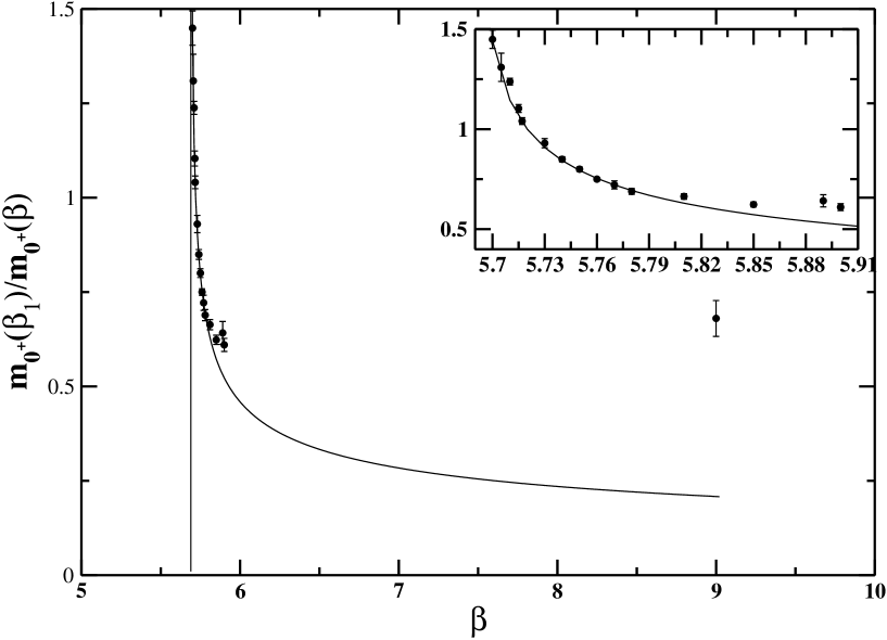
Figure 7: Comparison between the scaling function $[(\beta_{1}-\beta_{t})/(\beta-\beta_{t})]^{1/3}$ and the mass ratio $m_{0^{+}}(\beta_{1})/m_{0^{+}}(\beta)$ for varying $\beta$, with $\beta_{1}$=5.72.

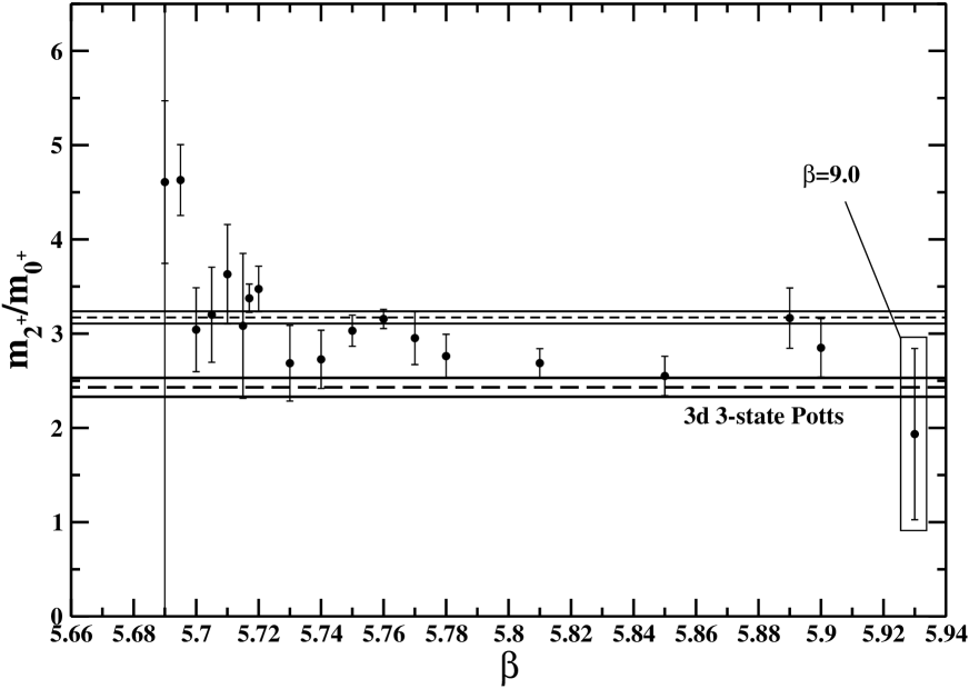
Figure 8: Ratio $m_{2}^{+}/m_{0}^{+}$ as a function of $\beta$ in the deconfined phase. The three upper horizontal lines represent the constant (with its error) which fits the data (see the text for details); the three lower horizontal lines represent the corresponding mass ratio (with its error) found in the 3$d$ 3-state Potts model [24].

3.2 Comparison with Polyakov loop models

We have calculated the ratio $m_{I}/m_{R}$ for $\beta$ ranging from 5.695 up to 9.0. We observe from Fig. 9 that this ratio is compatible with 3/2 at the largest $\beta$ values considered, in agreement with the high-temperature perturbation theory. Then, when the temperature is lowered towards the transition, this ratio goes up to a value compatible with 3, in agreement with the Polyakov loop model of Ref. [29], which contains only quadratic, cubic and quartic powers of the Polyakov loop, i.e. the minimum number of terms required in order to be compatible with a first order phase transition. The same trend has been observed also in Ref. [37].

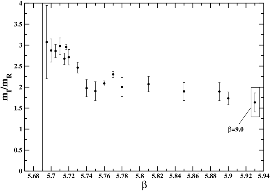
Figure 9: Ratio $m_{I}/m_{R}$ as a function of $\beta$ in the deconfined phase. The vertical line corresponds to the critical $\beta$ value.

4 Conclusions and outlook

In this work we have studied some screening masses of the (3+1)$d$ SU(3) pure gauge theory from Polyakov loop correlators in a large interval of temperatures above the deconfinement transition.

In particular, we have considered the lowest masses in the 0⁺ and the 2⁺ channels of angular momentum and parity and the screening masses resulting from the correlation between the real parts and between the imaginary parts of the Polyakov loop.

The behavior of the ratio between the masses in the 0⁺ and the 2⁺ channels with the temperature suggests that they have a common scaling above the transition temperature. This ratio turns to be $\simeq$30% larger than the ratio of the lowest massive excitations in the same channels of the 3$d$ 3-state Potts model in the broken phase. This can be taken as an estimate of the level of approximation by which the Svetitsky-Yaffe conjecture, valid in strict sense only for continuous phase transitions, can play some role also for (3+1)$d$ SU(3) at finite temperature.

The dependence on the temperature of the ratio between the screening masses from the correlation between the real parts and between the imaginary parts of the Polyakov loop shows a nice interplay between the high-temperature regime, where perturbation theory should work, and the transition regime, where mean-field effective Polyakov loop models could apply.

References

- [1] A.M. Polyakov, Phys. Lett. B 72 (1978) 477.
- [2] L. Susskind, Phys. Rev. D 20 (1979) 2610.
- [3] M. Fukugita, T. Kaneko and A. Ukawa, Phys. Lett. B 154 (1985) 185.
- [4] P. Bacilieri et al., Phys. Rev. Lett. 61 (1988) 1545.
- [5] F.R. Brown, N.H. Christ, Y. Deng, M. Gao and T.J. Woch, Phys. Rev. Lett. 61 (1988) 2058.
- [6] J. Kogut et al., Phys. Rev. Lett. 51, (1983) 869.
- [7] O. Kaczmarek, F. Karsch, E. Laermann and M. Lütgemeier, Phys. Rev. D 62 (2000) 034021.
- [8] R.V. Gavai, F. Karsch and B. Petersson, Nucl. Phys. B 322 (1989) 738.
- [9] B. Svetitsky and L.G. Yaffe, Nucl. Phys. B 210 (1982) 423.
- [10] F. Gliozzi and P. Provero, Phys. Rev. D 56 (1997) 1131.
- [11] R. Fiore, F. Gliozzi and P. Provero, Phys. Rev. D 58 (1998) 114502.
- [12] J. Engels and T. Scheideler, Nucl. Phys. B 539 (1999) 557.
- [13] S. Fortunato, F. Karsch, P. Petreczky and H. Satz, Nucl. Phys. (Proc. Suppl.) 94 (2001) 398.
- [14] R. Fiore, A. Papa and P. Provero, Nucl. Phys. (Proc. Suppl.) 106 (2002) 486.
- [15] R. Fiore, A. Papa and P. Provero, Phys. Rev. D 63 (2001) 117503.
- [16] A. Papa and C. Vena, Int. J. Mod. Phys. A 19 (2004) 3209.
- [17] A. Pelissetto and E. Vicari, Phys. Rept. 368 (2002) 549.
- [18] H.W.J. Blöte and R.H. Swendsen, Phys. Rev. Lett. 43 (1979) 779.
- [19] W. Janke and R. Villanova, Nucl. Phys. B 489 (1997) 679 and references therein.
- [20] M. Caselle, M. Hasenbusch and P. Provero, Nucl. Phys. B 556 (1999) 575.
- [21] M. Caselle, M. Hasenbusch, P. Provero and K. Zarembo, Nucl. Phys. B 623 (2002) 474.
- [22] R. Fiore, A. Papa and P. Provero, Nucl. Phys. (Proc. Suppl.) 119 (2003) 490.
- [23] R. Fiore, A. Papa and P. Provero, Phys. Rev. D 67 (2003) 114508.
- [24] R. Falcone, R. Fiore, M. Gravina and A. Papa, Nucl. Phys. B 767 (2007) 385.
- [25] R.D. Pisarski, Phys. Rev. D 62 (2000) 111501.
- [26] A. S. Kronfeld, Nucl. Phys. (Proc. Suppl.) 17 (1990) 313.
- [27] M. Lüscher and U. Wolff, Nucl. Phys. B 339 (1990) 222.
- [28] V. Agostini, G. Carlino, M. Caselle and M. Hasenbusch Nucl. Phys. B 484 (1997) 331.
- [29] A. Dumitru and R.D. Pisarski, Nucl. Phys. (Proc. Suppl.) 106 (2002) 483.
- [30] S. Nadkarni, Phys. Rev. D 33 (1986) 3738.
- [31] A. Dumitru and R.D. Pisarski, Phys. Rev. D 66 (2002) 096003.
- [32] N. Cabibbo and E. Berker, Phys. Lett. B 119 (1982) 387.
- [33] S.L. Adler, Phys. Rev. D 23 (1981) 2901.
- [34] G. Boyd, J. Engels, F. Karsch, E. Laermann, C. Legeland, M. Lutgemeier and B. Petersson, Nucl. Phys. B 469 (1996) 419.
- [35] S. Datta and S. Gupta, Nucl. Phys. B 534 (1998) 392 [arXiv:hep-lat/9806034].
- [36] B. Grossman, S. Gupta, U. M. Heller and F. Karsch, Nucl. Phys. B 417 (1994) 289 [arXiv:hep-lat/9309007].
- [37] S. Datta and S. Gupta, Phys. Rev. D 67 (2003) 054503 [arXiv:hep-lat/0208001].
- [38] M. E. Fisher and A. N. Berker, Phys. Rev. B 26 (1982) 2507.