Virtual Photon Emission from Quark-Gluon Plasma

Abstract

We recently proposed an empirical approach for the Landau-Pomeranchuk-Migdal (LPM) effects in photon emission from the quark gluon plasma as a function of photon mass. This approach was based on Generalized Emission Functions (GEF) for photon emission, derived at a fixed temperature and strong coupling constant. In the present work, we have extended the LPM calculations for several temperatures and strong coupling strengths. The integral equations for (${\bf\tilde{f}(\tilde{p}_{\perp})}$) and ($\tilde{g}({\bf\tilde{p}_{\perp}})$) are solved by the iterations method for the variable set {$p_{0},q_{0},Q^{2},T,\alpha_{s}$}, considering bremsstrahlung and $\bf aws$ processes. We generalize the dynamical scaling variables, $x_{T}$, $x_{L}$, for bremsstrahlung and aws processes which are now functions of variables $p_{0},q_{0},Q^{2},T,\alpha_{s}$. The GEF introduced earlier, $g^{b}_{T}$, $g^{a}_{T}$, $g^{b}_{L}$, $g^{a}_{L}$, are also generalized for any temperatures and coupling strengths. From this, the imaginary part of the photon polarization tensor as a function of photon mass and energy can be calculated as a one dimensional integral over these GEF and parton distribution functions in the plasma. However, for phenomenological studies of experimental data, one needs a simple empirical formula without involving parton momentum integrations. Therefore, we present a phenomenological formula for imaginary photon polarization tensor as a function of {$q_{0},Q^{2},T,\alpha_{s}$} that includes bremsstrahlung and $\bf aws$ mechanisms along with LPM effects.

In this work, we present a study of Landau-Pomeranchuk-Migdal effects landau1 ; migdal (LPM) in virtual photon emission from thermalized quark gluon plasma (QGP). The LPM effects on real photon emission from QGP have been reported arnold1 ; arnold2 and an empirical approach in svsprc . For the case of virtual photon emission in QGP, the processes that contribute at $\alpha\alpha_{s}$ order alther and the higher order corrections thoma and LPM effects lpmdilep were well studied. In hard thermal loops (HTL) braaten method these processes occur at the one loop, two lop and higher loop levels represented by ladder diagrams. In the photon emission calculations, the quantity of interest is the the imaginary part of photon retarded polarization tensor ($\Im{\Pi^{\mu}}_{R\mu}$). The dilepton emission rates are estimated in terms of this $\Im{\Pi^{\mu}}_{R\mu}$, Bose-Einstein factor and $Q^{2}$ as given by Eq.1. The $\Im{\Pi^{\mu}}_{R\mu}$ including LPM effects is determined in terms of a transverse function ${\bf{f}({{p}}_{\perp})}$ and a longitudinal part ${{g}({{p}}_{\perp})}$, as given by Eq.2 lpmdilep .

For the case of virtual photon emission having small virtuality, the transverse vector function ${\bf f({p}_{\perp}})$ is determined by the AMY equation (Eq.3) and the longitudinal function by AGMZ equation (Eq.4) lpmdilep . The energy transfer function $\delta{E}({\bf{p}_{\perp}},p_{0},q_{0},Q^{2},T,\alpha_{s})$ is given in Eq.5. The tilde represents quantities in units of Debye mass, for details see svsarxiv06 .

$$\frac{dN_{\ell^{+}\ell^{-}}}{d^{4}xd^{4}Q} = \frac{\alpha_{EM}}{12\pi^{4}Q^{2}(e^{q0/T}-1)}\Im\Pi_{R\mu}^{\mu}(Q)$$ (1)

$$\Im{\Pi^{\mu}}_{R\mu} = \frac{e^{2}N_{c}}{2\pi}\int_{-\infty}^{\infty}dp_{0}[n_{F}(r_{0})-n_{F}(p_{0})]\otimes$$ (2)

$$\int\frac{d^{2}{\bf{p}_{\perp}}}{(2\pi)^{2}}\left[\frac{p_{0}^{2}+r_{0}^{2}}{2(p_{0}r_{0})^{2}}\Re{\bf{p}_{\perp}.{f}({p}_{\perp})}+\right.$$

$$\left.\frac{1}{\sqrt{\left|p_{0}r_{0}\right|}}\frac{Q^{2}}{q^{2}}\Re{g}({\bf{p}_{\perp}})\right]$$

$$2{\bf\tilde{p}_{\perp}} = i\widetilde{\delta E}({\bf\tilde{p}_{\perp}},p_{0},q_{0},Q^{2}){\bf\tilde{f}}({\bf\tilde{p}_{\perp}})$$ (3)

$$+\int\frac{d^{2}{\bf\tilde{\bf\ell}_{\perp}}}{(2\pi)^{2}}\tilde{C}({\bf\tilde{\ell}_{\perp}})\left[{\bf\tilde{f}}({\bf\tilde{p}_{\perp}})-{\bf\tilde{f}}({\bf\tilde{p}_{\perp}+\tilde{\bf\ell}_{\perp}})\right]$$

$$2\sqrt{\frac{|p_{0}r_{0}|}{m_{D}^{2}}} = i\widetilde{\delta E}(({\bf\tilde{p}_{\perp}},p_{0},q_{0},Q^{2}){\tilde{g}}({\bf\tilde{p}_{\perp}})+$$ (4)

$$\int\frac{d^{2}{\bf\tilde{\ell}_{\perp}}}{(2\pi)^{2}}\tilde{C}({\bf\tilde{\ell}_{\perp}})\left[{\tilde{g}}({\bf\tilde{p}_{\perp}})-{\tilde{g}}({\bf\tilde{p}_{\perp}+\tilde{\bf\ell}_{\perp}})\right]~{}~{}~{}~{}~{}$$

$$\widetilde{\delta E} = \frac{q_{0}T}{2p_{0}(q_{0}+p_{0})}\left[\tilde{p}_{\perp}^{2}+\kappa_{\mbox{\small{eff}}}\right]$$ (5)

I Generalized Emission Functions for photon emission

In the present work, we solved these Eqs.(3,4) by iterations method at a fixed photon energy of ${q_{0}}$/T=50. Alternatively, these equations can also be solved by variational approach svsvar . In the following calculations, we have used two flavors and three colors. Using the iterations method, we obtained ${\bf p_{\perp}.f(p_{\perp})},g({\bf p_{\perp}})$ distributions for different $p_{0},q_{0},Q^{2}$, plasma temperatures (T=1.0, 0.50, 0.25GeV) and strong coupling constants ($\alpha_{s}$=0.30, 0.10, 0.05). We integrate these ${\bf p_{\perp}.f(p_{\perp})},g({\bf p_{\perp}})$ distributions to derive $I^{b,a}_{T,L}$ as defined in the Eqs.6,7. The superscripts $b,a$ in these equations represent bremsstrahlung or $\bf aws$ processes depending on the $p_{0}$ value used. The subscripts $T,L$ represent contributions from transverse ($\bf f(p_{\perp})$) or longitudinal $(g(\bf p_{\perp}))$ parts. $I^{b,a}_{T,L}$ are the quantities required for calculating imaginary part of polarization tensor (see Eq.2). Therefore, in the following, we empiricize these $I^{b,a}_{T,L}$.

$$I^{b,a}_{T} = \int\frac{\bf d^{2}\tilde{p}_{\perp}}{(2\pi)^{2}}{\bf\tilde{p}_{\perp}\cdot\Re\tilde{f}(\tilde{p}_{\perp})}$$ (6)

$$I^{b,a}_{L} = \int\frac{\bf d^{2}\tilde{p}_{\perp}}{(2\pi)^{2}}\Re\tilde{g}({\bf\tilde{p}_{\perp})}$$ (7)

$$x_{0} = \frac{|(p_{0}+q_{0})p_{0}|}{q_{0}T}~{};~{}x_{3}=\frac{q_{0}T(\alpha_{s}/0.3)}{Q^{2}}$$ (8)

$$x_{1} = x_{0}\frac{M_{\infty}^{2}}{m_{D}^{2}}$$ (9)

$$x_{2} = x_{0}\frac{Q^{2}}{q_{0}T(\alpha_{s}/0.3)}$$ (10)

$$x_{T} = x_{1}+x_{2}$$ (11)

$$x_{L} = x_{2}$$ (12)

$$g^{b,a}_{T,L}(x_{T,L}) = I^{b,a}_{T,L}(x_{T,L})c^{b,a}_{T,L}$$ (13)

In the remaining part of this work, we adopt the formulae and results of svsarxiv06 presented at fixed T=1GeV, $\alpha_{s}=0.30$, by suitably redefining the quantities for all temperatures and strong coupling constants. In Eqs.8,9,10 we define four dimensionless variables. The factor $\alpha_{s}/0.3$ in above equations is required to match the definitions in present work with those of svsarxiv06 . The variable $x_{1}$ is the real photon dynamical variable svsprc . For virtual photon emission from QGP, we define two more variables, $x_{T,L}$ given in Eqs.11,12. $I^{b,a}_{T,L}$ are in general functions of {$p_{0},q_{0},Q^{2},T,\alpha_{s}$} and when plotted versus any of these $p_{0},q_{0},Q^{2}$, they do not exhibit any simple trends. Following svsarxiv06 , we define the generalized emission functions (GEF) $g^{b,a}_{T,L}$ in Eq.13. The GEF are functions of only $x_{T,L}$ variables. These GEF ($g^{b,a}_{T,L}$) are obtained from corresponding $I^{b,a}_{T,L}$ values by multiplying with $c^{b,a}_{T,L}$ coefficient functions given in Eqs.14-18. The variable $x$ in Eqs.19-23 is $x_{T}$ for transverse part and $x_{L}$ for longitudinal parts. The quantities $x_{T,L}$ and $c^{b,a}_{T,L}$ in Eqs.11-18 are found by search for dynamical variables hidden in the solutions of AMY and AGMZ equations.

$$c^{b}_{T} = \frac{1}{x_{1}^{2}}$$ (14)

$$c^{a}_{T} = \frac{1}{x_{1}x_{2}}$$ (15)

$$c^{a}_{T} = \frac{1}{x_{1}^{2}}\frac{x_{3}}{1+x_{3}}~{}~{}~{}\mbox{for}~{}~{}~{}x_{2}<2.0$$ (16)

$$c^{b}_{L} = \frac{Q^{2}}{T^{2}(\alpha_{s}/0.3)}\left(\frac{T^{2}}{p_{0}(p_{0}+q_{0})}\right)^{\frac{3}{2}}\otimes$$ (17)

$$\frac{\left(1.5+x_{3}^{0.75}\right)}{x_{2}^{1/3}}\sqrt{\frac{\alpha_{s}}{0.3}}$$

$$c^{a}_{L} = \frac{x_{2}^{0.10}}{x_{1}^{1.40}\sqrt{q_{0}/T}\left(1+\sqrt{x_{3}}\right)}\sqrt{\frac{\alpha_{s}}{0.3}}$$ (18)

$$g^{b}_{T}(x) = \frac{10.0}{5.6+2.5\sqrt{x}+x}$$ (19)

$$g^{a}_{T}(x) = \frac{0.80}{(1+3/x^{1.2})}$$ (20)

$$g^{a}_{T}(x) = g^{b}_{T}(x)~{}~{}~{}\mbox{for}~{}~{}~{}x_{2}<2.0$$ (21)

$$g^{b}_{L}(x) = \frac{0.0876}{1+\left(\frac{x}{3.7727}\right)^{1.18}}$$ (22)

$$g^{a}_{L}(x) = 0.299803x^{0.5772}$$ (23)

$$g^{a}_{L}(x) = 1.04344\ln{(x)}~{}~{}~{}\mbox{for}~{}x>1.45$$

Figure 1 shows the results for GEF for bremsstrahlung (Fig.1(a)). The calculations are for a fixed photon energy ($q_{0}$/T=50.) but include six different cases of temperatures and coupling strengths mentioned in figure labels. The solid curve in (a) is the empirical fit to this emission function, given by Eq.19 . The required $c^{b}_{T}$ coefficient function is given in Eq.14. It has been observed that for low Q², i.e., $x_{2}<2.0$, transverse part of $\bf aws$ process behaves similar to the transverse bremsstrahlung function. Therefore, we transform the low Q² transverse part of $\bf aws$ process as given by Eq.16. The resulting emission function is shown in Fig. 1(b). The solid curve is given in Eq.21, which is same as solid curve in Fig. 1(a).
The emission function for high Q² values ($x_{2}>2.0$) for transverse part of $\bf aws$ process is shown in Figure 2. The $c^{a}_{T}$ and the emission function are given in Eqs.15,20. Similarly, Figures (3(a,b) show the longitudinal components of GEF for bremsstrahlung (Fig.(a)) and $\bf aws$ (Fig.(b)). The coeffiicient functions and GEF are given in Eqs.17,22,18,23. These transformation functions are very complex..

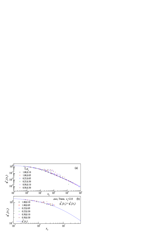
Figure 1: (a)  The dimensionless emission function $g^{b}_{T}(x)$ versus dynamical variable $x_{T}$ defined in Eq.11. Six cases of temperature and coupling constant values considered are mentioned in figure labels in different colored symbols. The symbols represent the integrated values of ${\bf p_{\perp}}$ distributions as a function of $\{p_{0},q_{0},Q^{2},T,\alpha_{s}\}$ values. These are transformed by $c^{b}_{T}$ coefficient function given in Eq.14. Essentially, various symbols merge and can not be distinguished. The solid curve is an empirical fit given by Eq.19. (b) The dimensionless emission function $g^{a}_{T}(x)$ versus dynamical variable $x_{T}$ for $x_{2}<2.0$. The transformation coefficients $c^{a}_{T}$ and empirical fit are given by Eqs.15,20.

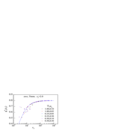
Figure 2: The dimensionless emission function $g^{a}_{T}(x)$ versus dynamical variable $x_{T}$. The symbols are as in figure 1. Six different temperature and coupling constant values considered are mentioned in figure labels. The required $c^{a}_{T}$ coefficient function given in Eq.LABEL:cath. The solid curve is an empirical fit given by Eq.19.

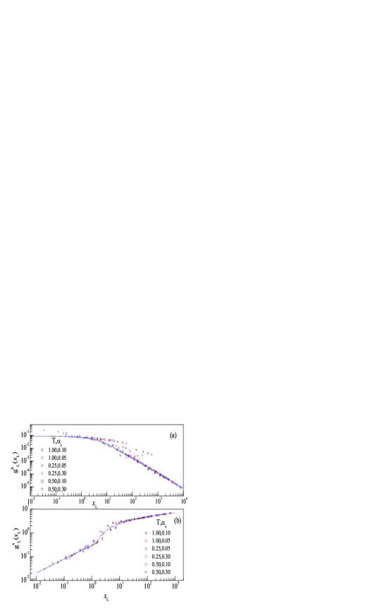
Figure 3: (a)  The dimensionless emission function $g^{b}_{L}(x)$ versus dynamical variable $x_{L}$ defined in Eq.12. The symbols represent the integrated values of ${\bf p_{\perp}}$ distributions as a function of $\{p_{0},q_{0},Q^{2},T,\alpha_{s}\}$ values. These are transformed by $c^{b}_{L}$ coefficient function given in Eq.17. The solid curve is an empirical fit given by Eq.22. The temperature and coupling constant values are mentioned in figure labels in different colors. (b) The dimensionless emission function $g^{a}_{L}(x)$ versus dynamical variable $x_{L}$. The transformation coefficients $c^{a}_{L}$ and empirical fit are given by Eqs.18,23.

II GEF and photon retarded polarization tensor

In the previous section, we used the results from the iterations methods to obtain the $I^{b,a}_{T,L}$ values by integrating the ${\bf p_{\perp}}$distributions. We transformed these into GEF ($g^{b,a}_{T,L}$) functions shown in Figs.1-3. We fitted these by empirical functions given in Eqs.19-23. Using the empirical functions, for any $p_{0},q_{0},Q^{2},T,\alpha_{s}$ values, we can generate the $I^{b,a}_{T,L}(x)$ values, circumventing the need to solve the integral equations. Thus, we have empiricized the $I^{b,a}_{T,L}$ values in terms of GEF. Hence, using GEF and the $c^{b,a}_{T,L}$, the imaginary part of photon retarded polarization tensor ($\Im\Pi_{R}$) is calculated, as in Eq.24 svsarxiv06 .

$$\Im{\Pi^{\mu}}_{R\mu} = \frac{e^{2}N_{c}}{2\pi}\int_{-\infty}^{\infty}dp_{0}[n_{F}(r_{0})-n_{F}(p_{0})]\otimes$$ (24)

$$\left(Tm_{D}^{2}\right)\left[\frac{p_{0}^{2}+r_{0}^{2}}{2(p_{0}r_{0})^{2}}\left(\frac{g^{i}_{T}\left(x_{T}\right)}{c^{i}_{T}}\right)+\right.$$

$$\left.\frac{1}{\sqrt{\left|p_{0}r_{0}\right|}}\frac{Q^{2}}{q^{2}}\left(\frac{1}{m_{D}}\right)\left(\frac{g^{i}_{L}\left(x_{L}\right)}{c^{i}_{L}}\right)\right]$$

Here, the superscript $i$ denotes $\{b,a\}$ depending on the value of the integration variable $p_{0}$. . We have calculated imaginary photon polarization tensor and dilepton emission rates using Eq.24 and made a detailed comparison with the results of lpmdilep . For this comparison, we generated reference results using the program provided by F. Gelis liblpm . The agreement of the GEF method of Eq.24 with the results of liblpm was observed to be very good. As an example, we show the dilepton emission rates in Figure 4. Figure shows the GEF results in symbols compared with the results of liblpm (blue lines) at a photon ${q_{0}}$/T=20.0 and $\alpha_{s}$=0.05 (see (a) ). The GEF results were generated using T=1.0GeV. Similarly in Figure (b) we show rates for $q_{0}$/T= 0.50 and $\alpha_{s}$=0.30 (in fig.(b)). The GEF results were generated at T=0.25GeV. The agreement of GEF method with lines is seen to be very good, except at the highest values of $\frac{Q}{T}$. This deviation is caused because for the longitudinal partin Eq.24, we used photon momentum $\frac{Q^{2}}{q^{2}}$. When this is replaced with photon energy $\frac{Q^{2}}{q_{0}^{2}}$ as shown in Eq.25, the agreement of our results with liblpm is very good in the full range of $Q/T$. In the remaining part of this paper, we use only Eq.25.

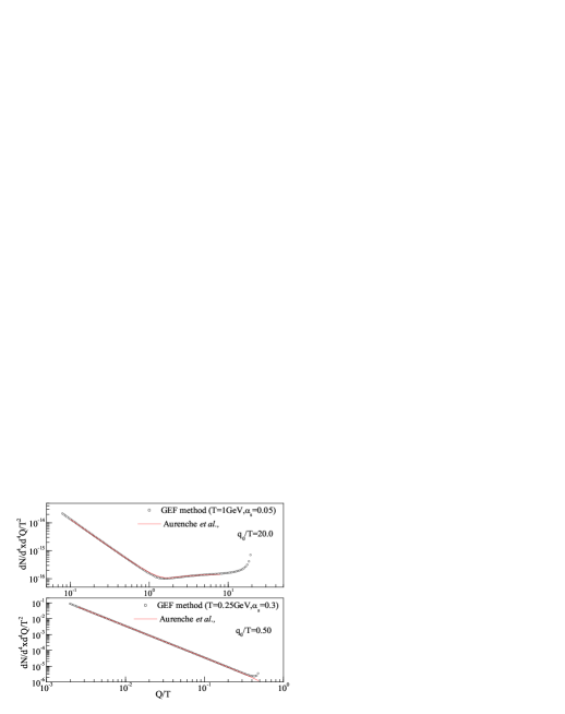
Figure 4: (a,b)  Dilepton emission rates using GEF method shown in symbols and compared with results of liblpm represented by blue lines. All the details are mentioned in figure labels and text.

$$\Im{\Pi^{\mu}}_{R\mu} = \frac{e^{2}N_{c}}{2\pi}\int_{-\infty}^{\infty}dp_{0}[n_{F}(r_{0})-n_{F}(p_{0})]\otimes$$ (25)

$$\left(Tm_{D}^{2}\right)\left[\frac{p_{0}^{2}+r_{0}^{2}}{2(p_{0}r_{0})^{2}}\left(\frac{g^{i}_{T}\left(x_{T}\right)}{c^{i}_{T}}\right)+\right.$$

$$\left.\frac{1}{\sqrt{\left|p_{0}r_{0}\right|}}\frac{Q^{2}}{q_{0}^{2}}\left(\frac{1}{m_{D}}\right)\left(\frac{g^{i}_{L}\left(x_{L}\right)}{c^{i}_{L}}\right)\right]$$

$$Q_{red} = \frac{Q}{T}\sqrt{\frac{0.3}{\alpha_{s}}}$$ (26)

$$\Im{\Pi_{red}} = \frac{\Im{\Pi^{\mu}}_{R\mu}(Q^{2},q_{0},T,\alpha_{s})}{T^{2}}\frac{0.30}{\alpha_{s}}$$ (27)

We will present more results in a different way by defining reduced quantities. After obtaining the $\Im{\Pi^{\mu}}_{R\mu}$ versus $Q^{2},q_{0},T,\alpha_{s}$ by using Eq.25, we define the reduced polarization tensor as and reduced Q_red as in Eqs.26,27. The reduced polarization tensors are calculated for different photon energies, different coupling strengths and temperatures. We plotted these results in balck circles in Figs.5,6 versus $Q_{red}$. For comparison, results from liblpm are shown in red symbols. The agreement of these two symbols is seen to be very good from low to very high photon energies, $q_{0}/T\sim 0.05-50.0$.

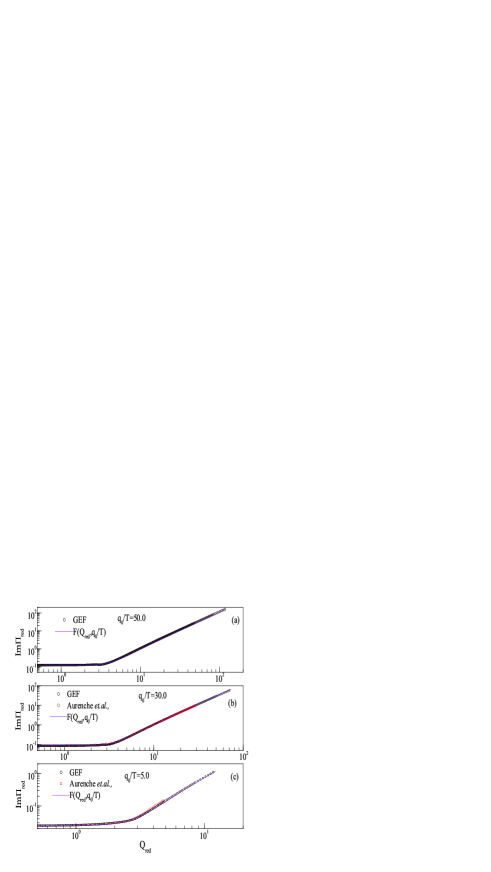
Figure 5: $\Im\Pi_{red}$ plotted as a function of $Q_{red}=\frac{Q}{T}\sqrt{\frac{0.3}{\alpha_{s}}}$ for various photon energies ($q_{0}/T$) mentioned in figure. The imaginary polarization tensor includes all contributions from transverse components of bremsstrahlung, $\bf aws$, and also from the corresponding longitudinal parts. The black circles represent the GEF method in Eq.25. The red circles represent the results of liblpm . The solid lines in violet color represent the results using Eq.30.

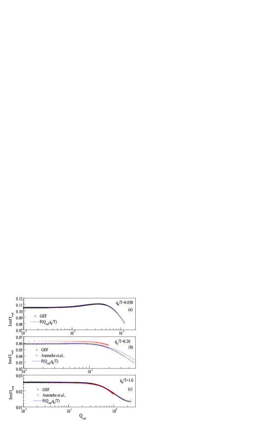
Figure 6: $\Im\Pi_{red}$ plotted as a function of $Q_{red}$ for low $q_{0}/T$ values mentioned in figure. The details are as in previous figure 5.

III Phenomenology using Generalized Emission Functions

In this section, we obtain the phenomenological fits to virtual photon emission rates from QGP. From the Figures 5,6, it is clear that the reduced quantities depend on only two variables, i.e., instead of {$Q^{2},q_{0},T,\alpha_{s}$}, we need only {$Q_{red},q_{0}/T$} to generate $\Pi_{red}$ as in Eq.28. This observation was already reported in lpmdilep .

$$\Im\Pi_{red}=F(Q_{red},\frac{q_{0}}{T})$$ (28)

In the limit of $Q_{red}\rightarrow 0$, $F(Q_{red},\frac{q_{0}}{T})\rightarrow F_{0}(\frac{q_{0}}{T}$). To study this further, we use Eq.25 to generate imaginary part of polarization tensor for various values of $Q^{2},q_{0},T,\alpha_{s}$. At first, we generate the $Im\Pi$ at a very low $Q^{2}$, $Q\sim 10^{-4}q_{0}$, for various values of $q_{0}/T,\alpha_{s}$. Using the results, we construct $Q_{red},\Im\Pi_{red}$. The results are shown in Figure 7 by symbols labeled GEF method. The results for different $\alpha_{s},T$ merge into a single curve in Fig.7. We fitted this data by suitable functions as given in Eqs.31 along with their parameters. These are two different fits, one for $q_{0}/T<$200 and the other for $q_{0}/T>$100, with an overlap between 100-200. These are represented by solid curves and labeled $F_{0}$ in figure. The $\Im\Pi_{red}$ below $q_{0}/T<0.020$ is approximately equal to this function $F_{0}$, as given by Eq.29. However, it should be noted that at ultra soft photon energies, the present formalism needs corrections moore .

For the case of finite $Q^{2}$, we made empirical fits by choosing a function given in Eq.30. In this function, A,B,C parameters are function of $q_{0}/T$ and are determined by fitting the $Q^{2}$ plots for various $q_{0}/T$. These parameters values for various $q_{0}/T$ are tabulated and are shown in Figure 8. It is very important to have an empirical formula to generate A,B,C values. Therefore, these A,C,B parameters were fitted by different functional forms as given in Eqs.33,36,38. The parameters are different for different $q_{0}/T$ regions. Therefore, depending on the requirement, one can select the relevant parameter set to generate A,B,C values. Using these formulae we get A,B,C coefficients and we get F${}_{0}(x)$ from Eq.31. We use these in Eq.30 to generate $\Im\Pi_{red}$. These phenomenological results are shown by solid curves in Figs.5,6.

$$F(Q_{red},x) \approx F_{0}(x)~{}~{}\mbox{for}~{}~{}x\leq 0.020$$ (29)

$$x = \frac{q_{0}}{T}$$

$$F(Q_{red},x) = F_{0}(x)\frac{(1+A(x)Q_{red}+B(x)Q_{red}^{4})}{(1+C(x)Q_{red}^{2})}$$ (30)

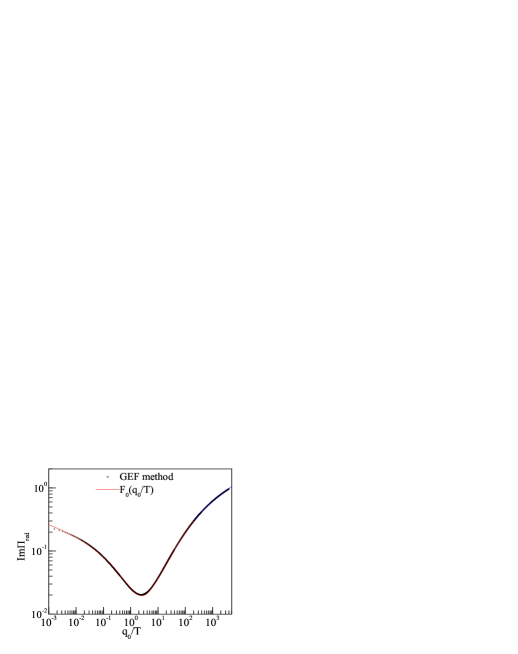
Figure 7: The reduced imaginary part of polarization tensor defined in Eq.27, versus $q_{0}/T$. We have taken as $Q\sim 10^{-4}q_{0}$. The solid curves are fits given in Eq.31. The symbols represent the results from GEF method using Eq.25.

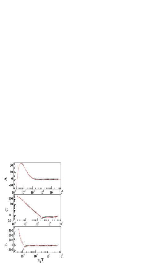
Figure 8: The A,B,C parameters versus $q_{0}/T$. The curves represent fits by suitable functional forms in Eqs.33, 36, 38 discussed in text. These are useful to generate $\Pi_{red}$ using Eq.30. Apparently, at high $q_{0}/T$, these parameters are constant, however this is very misleading. The present fits generate quite well the small variations of these parameters over full region. Good quality A,B,C fits are required because, the $Q^{2}$ plots are sensitive to these parameters ane there is delicate cancellation of various terms in Eq.30.

$$F_{0}(x) = a+bx^{p_{1}}+\frac{c}{\sqrt{x^{p_{2}}}}~{}~{}\mbox{for}~{}x\leq 200.$$ (31)

$$a = -2.99077$$

$$b = 0.0791399$$

$$c = 2.93755$$

$$p_{1} = 0.371976$$

$$p_{2} = 0.0288541$$

$$F_{0}(x) = a+b\sqrt{x^{p}}~{}~{}\mbox{for}~{}~{}x\geq 100.0$$ (32)

$$a = -0.474129$$

$$b = 0.255163$$

$$p = 0.419646$$

$$A(x) = a+(bx^{p_{1}}-cx^{p_{2}})~{}~{}\mbox{for}~{}~{}x\leq 0.1$$ (33)

$$a = -4.84554727516$$

$$b = 1.478772613744$$

$$c = 0.4963049612794$$

$$p_{1} = -0.93213485133$$

$$p_{2} = -1.1101191721$$

$$A(x) ~{}~{}\mbox{for}~{}0.1<x\leq 3.5$$ (34)

$$a = 0.33219586043$$

$$b = 1.34926189543$$

$$c = 1.82125018461$$

$$p_{1} = -1.0422409717$$

$$p_{2} = -0.86799168105$$

$$A(x) = A(3.5)~{}~{}\mbox{for}~{}~{}x>3.50$$ (35)

$$C(x) = a+(bx^{p_{1}}-cx^{p_{2}})~{}~{}\mbox{for}~{}~{}x\leq 0.15$$ (36)

$$a = 7.48658946052$$

$$b = 13.1687711578$$

$$c = 19.9115694165$$

$$p_{1} = -1.0750505095$$

$$p_{2} = -0.8514587339$$

$$C(x) ~{}~{}~{}~{}\mbox{for}~{}~{}x>0.15$$ (37)

$$a = 0.0692890486$$

$$b = 0.945340977$$

$$c = 0.8057948943$$

$$p_{1} = -1.4427187803$$

$$p_{2} = -1.2054627582$$

$$B(x) = a+(bx^{p_{1}}-cx^{p_{2}})~{}~{}\mbox{for}~{}~{}x\leq 0.20$$ (38)

$$a = -0.132747$$

$$b = 0.0661859$$

$$c = 0.0642336$$

$$p_{1} = -4.76869$$

$$p_{2} = -4.77762$$

$$B(x) ~{}~{}\mbox{for}~{}0.2<x\leq 1.0$$ (39)

$$a = 0.012385$$

$$b = 0.0924141$$

$$c = 0.0878252$$

$$p_{1} = -4.18536$$

$$p_{2} = -4.25575$$

$$B(x) ~{}~{}\mbox{for}~{}~{}~{}x>1.0$$ (40)

$$a = -0.0454930477$$

$$b = 0.1940150437$$

$$c = 0.1372510415$$

$$p_{1} = -0.237037465$$

$$p_{2} = -0.42563026$$

In conclusion, the photon emission rates from the quark gluon plasma have been studied as a function of photon mass, considering LPM effects at various temperatures and strong coupling strengths. We defined generalized dynamical variables $x_{T},x_{L}$ for transverse and longitudinal components of bremsstrahlung and $\bf aws$ mechanism. In addition, we defined generalized emission functions (GEF) namely $g^{b}_{T}(x_{T})$,$g^{a}_{T}(x_{T})$,$g^{b}_{L}(x_{L})$,$g^{a}_{L}(x_{L})$. We have obatined empirical fits to these GEF. In terms of the GEF, we have calculated the imaginary part of retarded photon polarization tensor as a function of photon energy and mass, plasma temperature and strong coupling strengths. For phenomenological applications, we fitted the reduced imaginary polarization tensor by simple functions and provided necessary parameters.