Quantum Hall ferromagnetism in graphene: an SU(4) bosonization approach

Abstract

We study the quantum Hall effect in graphene at filling factors $\nu=0$ and $\nu=\pm 1$, concentrating on the quantum Hall ferromagnetic regime, within a non-perturbative bosonization formalism. We start by developing a bosonization scheme for electrons with two discrete degrees of freedom (spin-1/2 and pseudospin-1/2) restricted to the lowest Landau level. Three distinct phases are considered, namely the so-called spin-pseudospin, spin, and pseudospin phases. The first corresponds to a quarter-filled ($\nu=-1$) while the others to a half-filled ($\nu=0$) lowest Landau level. In each case, we show that the elementary neutral excitations can be treated approximately as a set of $n$-independent kinds of boson excitations. The boson representation of the projected electron density, the spin, pseudospin, and mixed spin-pseudospin density operators are derived. We then apply the developed formalism to the effective continuous model, which includes SU(4) symmetry breaking terms, recently proposed by Alicea and Fisher. For each quantum Hall state, an effective interacting boson model is derived and the dispersion relations of the elementary excitations are analytically calculated. We propose that the charged excitations (quantum Hall skyrmions) can be described as a coherent state of bosons. We calculate the semiclassical limit of the boson model derived from the SU(4) invariant part of the original fermionic Hamiltonian and show that it agrees with the results of Arovas and co-workers for SU(N) quantum Hall skyrmions. We briefly discuss the influence of the SU(4) symmetry breaking terms in the skyrmion energy.

I Introduction

Graphene consists of a single atomic layer of carbon arranged in a honeycomb lattice.ando ; castroneto06 When an uniform perpendicular magnetic field is applied, the system displays an unconventional integer quantum Hall effect (QHE),geim ; kim where the Hall conductivity $\sigma_{xy}=4(n+1/2)e^{2}/h$ ($n$ integer) and the filling factor is defined as $\nu=4(n+1/2)$. Such unusual behavior of $\sigma_{xy}$ is understood within a single-particle modelgusynin ; castroneto06 which shows that each Landau level in graphene is approximately four-fold degenerate (valley, the so-called $\mathbf{K}$ and $\mathbf{K^{\prime}}$ points, and electron spin).

More interesting, experiments performed at higher magnetic fields showed new quantum Hall plateaus at $\nu=0,\,\pm 1$, and $\pm 4$,zhang06 indicating that the degeneracies of the $n=0$ and $n=1$ Landau levels are lifted. In particular, for $\nu=\pm 4$, the behavior of the minimum of the longitudinal resistance $R_{xx}$ in terms of the total magnetic field suggests that here the quantum Hall effect is due to the lifting of the spin degeneracy of the $n=1$ Landau level.zhang06 However, the origin of the plateaus at $\nu=0$ and $\nu=\pm 1$ is not completely understood. Different scenarios were proposed. It was suggested that the effect is due to Coulomb interaction, which favors a quantum Hall ferromagnet ground state.nomura06 Alicea and Fisheralicea06 proposed that the plateaus might be related to symmetry breaking terms, such as Zeeman and underlying lattice interactions, which give rise to a paramagnetic phase as it occurs at $\nu=\pm 4$. An explanation based on the so-called ”magnetic catalysis” mechanism was proposed by Gusynin et al.gusynin07 This mechanism predicts that the long-range Coulomb interaction generates an excitonic gap, which lifts the valley degeneracy only of the lowest Landau level. In combination with the Zeeman splitting, the observed quantum Hall plateaus at $\nu=0$ and $\pm 1$ are understood. More recently, Abanin et al.abanin07 argued that the transport response of the quantum Hall state at $\nu=0$ is due to counter-circulating edge states.

In this paper, we study the quantum Hall ferromagnetism in graphene via a non-perturbative bosonization method for the case of electrons with spin-1/2 and pseudospin-1/2 restricted to the lowest Landau level. It constitutes a generalization of the formalismdoretto recently proposed by one of us to study the two-dimensional electron gas at $\nu=1$ realized in GaAs heterostructures.perspectives ; yoshioka Within this formalism, the elementary neutral excitations (magnetic excitons) and the skyrmion-antiskyrmion pair excitations of the system are described in the same framework, namely an effective interacting boson model. Such method is quite general and was used to calculate spin excitations of the fractional quantum Hall systems at $\nu=1/3$ and $\nu=1/5$,doretto05 as well as to study Bose-Einstein condensation of magnetic excitons in the bilayer quantum Hall system at total filling factor $\nu_{T}=1$ (spinless case).doretto06

Concerning the latter, the great majority of models proposed to study this system assumes fully spin-polarized electrons. However, nuclear magnetic resonance measurementsspielman05 ; kumada05 indicate that the electron spin degree of freedom might be relevant. Indeed, it was suggested that the incompressible-compressible phase transition observed in this system may involve a modification of the spin polarization.spielman05 Therefore, theoretical tools which allow us to properly treat the electron-electron interaction and simultaneously take into account the electron spin and layer (pseudospin) degrees of freedom are needed. The formalism developed here might be also useful to study the bilayer quantum Hall system at $\nu_{T}=1$ in GaAs heterostructures (spinfull case).

Our paper is organized as follows. In Sec. II, we define the creation and annihilation boson operators and derive the boson representation of the (projected) electron density, spin, pseudospin, and mixed spin-pseudospin density operators. Three distinct cases are considered, the so-called spin-pseudospin phase, which occurs when the lowest Landau level is quarter-filled, the spin and pseudospin phases, which are related to a half-filled lowest Landau level. In Sec. III, we apply the generalized bosonization formalism to study the QHE in graphene at $\nu=0$ and $\nu=\pm 1$, focusing on the quantum Hall ferromagnetic regime. Our starting point is the effective continuous model recently proposed by Alicea and Fisher.alicea06 For each quantum Hall state, an effective interacting boson model is derived and the dispersion relations of the elementary neutral excitations are analytically calculated. We comment on some possible effects of the boson-boson interaction and show how the quantum Hall skyrmion might be described within this scheme. A summary of the main results is presented in Sec. IV.

II The bosonization method

In order to develop a bosonization scheme for electrons with two discrete degrees of freedom (spin-1/2 and pseudospin-1/2) and restricted to the lowest Landau level subspace, we follow the lines of Ref. doretto, and start by studying the corresponding noninteracting model.

Let us consider ${\rm N}$ noninteracting electrons moving in the $xy$ plane under a perpendicular magnetic field ${\bf B}=B\hat{z}$. In addition to the electronic spin ($\sigma$, $\lambda=\uparrow$, $\downarrow$), let us also include a discrete pseudospin index $\alpha$, $\beta=\pm$. Restricting the Hilbert space to the lowest Landau level, the kinetic energy is quenched and therefore the Hamiltonian of the system is

$$\mathcal{H} = \mathcal{H_{Z}}+\mathcal{H_{PZ}}$$

$$= -\frac{1}{2}\sum_{\sigma,\alpha}\int d^{2}r\;\left(\sigma E_{Z}+\alpha E_{P}\right)\Psi^{\dagger}_{\alpha\,\sigma}({\bf r})\Psi_{\alpha\,\sigma}({\bf r}).$$

In addition to the Zeeman term $\mathcal{H_{Z}}$, we also include an extra term ($\mathcal{H_{PZ}}$) which breaks the pseudospin degeneracy. As we will see below, a finite $E_{P}$ helps us to define a set of different reference states. $E_{Z}=g\mu_{B}B$ is the Zeeman energy, where $g$ is the effective electron $g$-factor and $\mu_{B}$ is the Bohr magneton (see Appendix A). $\Psi^{\dagger}_{\alpha\,\sigma}({\bf r})$ is a fermion field operator that can be expanded in the (Schrödinger) lowest Landau level basis $|n=0\,m\,\rangle$ (symmetric gauge)doretto as

$$\Psi^{\dagger}_{\alpha\,\sigma}({\bf r}) = \sum_{m}\langle n=0\,m\,|{\bf r}\rangle c^{\dagger}_{m\,\alpha\,\sigma},$$

$$\Psi_{\alpha\,\sigma}({\bf r}) = \sum_{m}\langle{\bf r}|n=0\,m\,\rangle c_{m\,\alpha\,\sigma}.$$ (2)

The operator $c^{\dagger}_{m\,\alpha\,\sigma}$ ($c_{m\,\alpha\,\sigma}$) creates (destroys) an electron in the lowest Landau level, with guiding center $m$, pseudospin $\alpha$, and spin $\sigma$. Substituting Eq. (2) into Eq. (II), one sees that the Hamiltonian $\mathcal{H}$ is diagonal in the lowest Landau level basis, i.e.,

$$\mathcal{H}=-\frac{1}{2}\sum_{m=0}^{{\rm N_{\phi}}-1}\sum_{\alpha,\sigma}\left(\sigma E_{Z}+\alpha E_{P}\right)c^{\dagger}_{m\,\alpha\,\sigma}c_{m\,\alpha\,\sigma}.$$ (3)

The above Hamiltonian has four highly degenerate energy levels, whose energies are $-(E_{Z}+E_{P})/2$, $-(E_{Z}-E_{P})/2$, $(E_{Z}-E_{P})/2$ and $(E_{Z}+E_{P})$, and the degeneracy of each level is ${\rm N_{\phi}}=1/2\pi l^{2}$. Here, $l=\sqrt{\hbar c/eB}$ is the magnetic length and we assume that the total area of the system is one. In the following, we will concentrate on three distinct configurations of the system: total number of electrons ${\rm N}={\rm N_{\phi}}$ and $E_{Z}>E_{P}$, which we call spin-pseudospin phase; ${\rm N}=2{\rm N_{\phi}}$ and $E_{Z}>E_{P}$ (spin phase); and ${\rm N}=2{\rm N_{\phi}}$ and $E_{Z}<E_{P}$ (pseudospin phase).

As discussed in Ref. doretto, , the creation and annihilation boson operators are defined by considering the neutral (particle-hole) excitations above a well-defined reference state. As each one of the above phases has a different reference state (noninteracting ground state), the three cases will be analyzed separately. However, before doing that, we should firstly discuss the representation and the algebra of the electron density, spin, pseudospin and mixed spin-pseudospin density operators projected into the lowest Landau level.

II.1 Density operators and the lowest Landau level algebra

We start by defining the following projected density operator

$$\rho_{\alpha\sigma,\beta\lambda}({\bf r})=\Psi^{\dagger}_{\alpha\sigma}({\bf r})\Psi_{\beta\lambda}({\bf r}),$$ (4)

where the fermion field operators are given by Eq. (2), and whose Fourier transform is

$$\rho_{\alpha\sigma,\beta\lambda}({\bf q}) = \int d^{2}r\;e^{-i\mathbf{q}\cdot\mathbf{r}}\Psi^{\dagger}_{\alpha\sigma}({\bf r})\Psi_{\beta\lambda}({\bf r})$$ (5)

$$= \sum_{m,m^{\prime}}\int d^{2}r\;e^{-i\mathbf{q}\cdot\mathbf{r}}\langle m|\mathbf{r}\rangle\langle\mathbf{r}|m^{\prime}\rangle c^{\dagger}_{m\,\alpha\,\sigma}c_{m^{\prime}\,\beta\,\lambda}$$

$$= e^{-(lq)^{2}/2}\sum_{m,m^{\prime}}G_{m,m^{\prime}}(l{\bf q})c^{\dagger}_{m\,\alpha\,\sigma}c_{m^{\prime}\,\beta\,\lambda},$$

with $q=|{\bf q}|$. The function $G_{m,m^{\prime}}(x)$ is defined as

$$G_{m,m^{\prime}}(l{\bf q}) = \theta(m^{\prime}-m)\sqrt{\frac{m!}{m^{\prime}!}}\left(\frac{-il(q_{x}-iq_{y})}{\sqrt{2}}\right)^{m^{\prime}-m}$$ (6)

$$\times L^{m^{\prime}-m}_{m}\left((lq)^{2}/2\right)$$

$$+ \theta(m-m^{\prime})\sqrt{\frac{m^{\prime}!}{m!}}\left(\frac{-il(q_{x}+iq_{y})}{\sqrt{2}}\right)^{m-m^{\prime}}$$

$$\times L^{m-m^{\prime}}_{m^{\prime}}\left((lq)^{2}/2\right),$$

where $L^{m-m^{\prime}}_{m^{\prime}}(x)$ is the generalized Laguerre polynomial.arfken Due to the fact that the operators $\rho_{\alpha\sigma,\beta\lambda}({\bf q})$ are projected into the lowest Landau level, their commutation relations are modified, i.e,

$$\left[\rho_{\alpha\sigma,\beta\lambda}({\bf q})\right. \left.\rho_{\alpha^{\prime}\sigma^{\prime},\beta^{\prime}\lambda^{\prime}}({\bf q}^{\prime})\right]=e^{{\bf q}\cdot{\bf q}^{\prime}l^{2}/2}$$ , (7)

$$\times \left[\delta_{\beta,\alpha^{\prime}}\delta_{\lambda,\sigma^{\prime}}e^{i{\bf q}\wedge{\bf q}^{\prime}/2}\rho_{\alpha\sigma,\beta^{\prime}\lambda^{\prime}}({\bf q}+{\bf q}^{\prime})\right.$$

$$- \left.\delta_{\alpha,\beta^{\prime}}\delta_{\sigma,\lambda^{\prime}}e^{-i{\bf q}\wedge{\bf q}^{\prime}/2}\rho_{\alpha^{\prime}\sigma^{\prime},\beta\lambda}({\bf q}+{\bf q}^{\prime})\right],$$

where ${\bf q}\wedge{\bf k}\equiv l^{2}({\bf q}\times{\bf k})\cdot\hat{z}$.

It is convenient to introduce an isospin index $I$ such that

$$I=(\alpha,\,\sigma)=(+,\uparrow),\,(+,\downarrow),\,(-,\uparrow),\,(-,\downarrow)=1,2,3,4.$$

In this new representation, the commutator (7) simply reads

$$[\rho_{IJ}({\bf q}),\rho_{\bar{I}\bar{J}}({\bf q}^{\prime})] = e^{{\bf q}\cdot{\bf q}^{\prime}l^{2}/2}\left[\delta_{J,\bar{I}}e^{i{\bf q}\wedge{\bf q}^{\prime}/2}\rho_{I\bar{J}}({\bf q}+{\bf q}^{\prime})\right.$$ (8)

$$-\left.\delta_{I,\bar{J}}e^{-i{\bf q}\wedge{\bf q}^{\prime}/2}\rho_{\bar{I}J}({\bf q}+{\bf q}^{\prime})\right].$$

It is also useful to define a four-component spinor $\hat{\Psi}^{\dagger}({\bf r})$ as

$$\hat{\Psi}^{\dagger}({\bf r}) = \left(\Psi^{\dagger}_{+\uparrow}({\bf r})\;\;\Psi^{\dagger}_{+\downarrow}({\bf r})\;\;\Psi^{\dagger}_{-\uparrow}({\bf r})\;\;\Psi^{\dagger}_{-\downarrow}({\bf r})\right),$$ (9)

which, in the isospin language, assumes the form

$$\hat{\Psi}^{\dagger}({\bf r}) = \left(\Psi^{\dagger}_{1}({\bf r})\;\;\Psi^{\dagger}_{2}({\bf r})\;\;\Psi^{\dagger}_{3}({\bf r})\;\;\Psi^{\dagger}_{4}({\bf r})\right).$$ (10)

The (projected) electron density operator can now be written in terms of the spinor (10) as

$$\rho({\bf r})=\hat{\Psi}^{\dagger}({\bf r})\hat{\Psi}({\bf r})=\sum_{I=1}^{4}\Psi^{\dagger}_{I}({\bf r})\Psi_{I}({\bf r})$$ (11)

and therefore its Fourier transform may be expressed in terms of the density operators $\rho_{IJ}({\bf q})$ as

$$\rho({\bf q})=\left[\rho_{11}({\bf q})+\rho_{22}({\bf q})+\rho_{33}({\bf q})+\rho_{44}({\bf q})\right].$$ (12)

The same can be done for the spin-$\sigma$ and pseudospin-$\alpha$ electron density operators

$$\rho_{\uparrow}({\bf q}) = \rho_{11}({\bf q})+\rho_{33}({\bf q}),\;\;\;\;\rho_{\downarrow}({\bf q})=\rho_{22}({\bf q})+\rho_{44}({\bf q}),$$

$$\rho_{+}({\bf q}) = \rho_{11}({\bf q})+\rho_{22}({\bf q}),\;\;\;\;\rho_{-}({\bf q})=\rho_{33}({\bf q})+\rho_{44}({\bf q}).$$

The definition (10) implies that the structure of the spin-pseudospin space is $SU(2)_{PS}\otimes SU(2)_{SPIN}$ and therefore, the spin, pseudospin, and mixed spin-pseudospin density operators ($\hbar=1$) are respectively defined as

$${\bf S}({\bf r})=\frac{1}{2}\hat{\Psi}^{\dagger}({\bf r})\left({\mathbf{1}}_{2\times 2}\otimes\hat{\sigma}\right)\hat{\Psi}({\bf r}),$$ (14)

$${\bf P}({\bf r})=\frac{1}{2}\hat{\Psi}^{\dagger}({\bf r})\left(\hat{\sigma}\otimes{\mathbf{1}}_{2\times 2}\right)\hat{\Psi}({\bf r}),$$ (15)

$${\bf P}{\bf S}({\bf r})=\frac{1}{2}\hat{\Psi}^{\dagger}({\bf r})\left(\hat{\sigma}\otimes\hat{\sigma}\right)\hat{\Psi}({\bf r}),$$ (16)

Here, ${\mathbf{1}}_{2\times 2}$ is the two-dimensional unit matrix and $\hat{\sigma}=(\sigma_{x}\;\;\sigma_{y}\;\;\sigma_{z})$ is a vector whose components are the Pauli matrices. Expanding the Fourier transform of the components of ${\bf S}({\bf r})$ and ${\bf P}({\bf r})$ in terms of the density operators $\rho_{IJ}({\bf q})$, we have

$$S_{\rm Z}({\bf q})=\frac{1}{2}\left[\rho_{11}({\bf q})-\rho_{22}({\bf q})+\rho_{33}({\bf q})-\rho_{44}({\bf q})\right],$$

$$S^{+}({\bf q})=[S_{\rm X}({\bf q})+iS_{\rm Y}({\bf q})]=\rho_{12}({\bf q})+\rho_{34}({\bf q}),$$ (17)

$$S^{-}({\bf q})=[S_{\rm X}({\bf q})-iS_{\rm Y}({\bf q})]=\rho_{21}({\bf q})+\rho_{43}({\bf q}),$$

and

$$P_{\rm Z}({\bf q})=\frac{1}{2}\left[\rho_{11}({\bf q})+\rho_{22}({\bf q})-\rho_{33}({\bf q})-\rho_{44}({\bf q})\right],$$

$$P^{+}({\bf q})=\rho_{13}({\bf q})+\rho_{24}({\bf q}),$$ (18)

$$P^{-}({\bf q})=\rho_{31}({\bf q})+\rho_{42}({\bf q}).$$

Similar considerations hold for the mixed operators ${\bf P}{\bf S}({\bf r})$, in particular, we have

$$P_{\rm Z}S_{\rm Z}({\bf q})=\frac{1}{2}\left[\rho_{11}({\bf q})-\rho_{22}({\bf q})-\rho_{33}({\bf q})+\rho_{44}({\bf q})\right].$$ (19)

This component of ${\bf P}{\bf S}({\bf q})$ will be important in the next sections. We should mention that the representation (14)-(16) does not correspond to the standard representation of the special unitary group SU(4) [see Ref. greiner, for details], but it follows the ideas presented in the Appendix A of Ref. ezawa04, .

Finally, with the aid of the commutator (8), a long but straightforward calculation shows that the density operators (12), (14) and (15) obey the lowest Landau level algebra (the same results have been derived in a more general waymark-notes )

$$\left[\rho({\bf q}),\rho({\bf k})\right] = 2i\sin\left({\bf q}\wedge{\bf k}/2\right)e^{{\bf q}\cdot{\bf k}/2}\rho({\bf q}+{\bf k}),$$

$$\left[I^{\mu}_{a}({\bf q}),\rho({\bf k})\right] = 2i\sin\left({\bf q}\wedge{\bf k}/2\right)e^{{\bf q}\cdot{\bf k}/2}I^{\mu}_{a}({\bf q}+{\bf k}),$$

$$\left[I^{\mu}_{a}({\bf q}),I^{\mu}_{b}({\bf k})\right] = (i/2)\delta_{a,b}\sin\left({\bf q}\wedge{\bf k}/2\right)e^{{\bf q}\cdot{\bf k}/2}\rho({\bf q}+{\bf k})$$

$$+ i\epsilon^{abc}\cos\left({\bf q}\wedge{\bf k}/2\right)e^{{\bf q}\cdot{\bf k}/2}I^{\mu}_{c}({\bf q}+{\bf k}),$$

$$\left[P_{a}({\bf q}),S_{b}({\bf k})\right] = i\sin\left({\bf q}\wedge{\bf k}/2\right)e^{{\bf q}\cdot{\bf k}/2}P_{a}S_{b}({\bf q}+{\bf k}).$$ (20)

Here, $a,b,c={\rm X,Y,Z}$ and $\epsilon^{abc}$ is the Levi-Civita tensor.arfken $\mu=S,P$ and therefore $I^{S}_{a}({\bf q})$ and $I^{P}_{a}({\bf q})$ stand respectively for $S_{a}({\bf q})$ and $P_{a}({\bf q})$. Due to the fact that the density operators (12), (14), and (15) are projected into the lowest Landau level, the algebra (20) is different from the usual one of the generators of the SU(4) group. greiner ; ezawa04

II.2 Spin-pseudospin polarized state

Let us now study the noninteracting system described by the Hamiltonian (3), assuming that the total number of electrons ${\rm N}={\rm N_{\phi}}$ and $E_{Z}>E_{P}$. The four (highly degenerate) energy levels are schematically displayed in Fig. 1. In this case, the noninteracting ground state of the system is a spin-polarized pseudospin-polarized state,

$$|{\rm SPFM}\rangle=\prod_{m=0}^{{\rm N_{\phi}}-1}c^{\dagger}_{m\,+\,\uparrow}|0\rangle,$$ (21)

where $|0\rangle$ is the fermion vacuum. Notice that the neutral (particle-hole) excitations are created by applying the density operators $\rho_{21}({\bf q})$, $\rho_{31}({\bf q})$, and $\rho_{41}({\bf q})$ on the state $|{\rm SPFM}\rangle$.

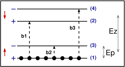
Figure 1: (color online) Schematic representation of the four highly degenerate lowest Landau levels when $E_{Z}>E_{P}$. The state $|{\rm SPFM}\rangle$ is obtained by completely filling the energy level (1). b1, b2 and b3 are the elementary neutral excitations which are related to the density operators $\rho_{21}({\bf q})$, $\rho_{31}({\bf q})$, and $\rho_{41}({\bf q})$, respectively.

From Eq. (8), it follows that the commutator between each one of the above density operators and its respective Hermitian conjugate is

$$[\rho_{1I}({\bf q}),\rho_{I1}({\bf q}^{\prime})] = e^{{\bf q}\cdot{\bf q}^{\prime}l^{2}/2}\left[e^{i{\bf q}\wedge{\bf q}^{\prime}/2}\rho_{11}({\bf q}+{\bf q}^{\prime})\right.$$ (22)

$$-\left.e^{-i{\bf q}\wedge{\bf q}^{\prime}/2}\rho_{II}({\bf q}+{\bf q}^{\prime})\right],$$

with $I=2,3,4$. By expanding the density operators $\rho_{II}({\bf q})$ around the (reference) state (21),

$$\rho_{II}({\bf q}) = \langle{\rm SPFM}|\rho_{II}({\bf q})|{\rm SPFM}\rangle+\delta\rho_{II}({\bf q})$$ (23)

$$= {\rm N_{\phi}}\delta_{I,1}\delta_{{\bf q},0}+\delta\rho_{II}({\bf q}),$$

and neglecting the fluctuations with respect to the average value, the commutator (22) assumes the form

$$[\rho_{1I}({\bf q}),\rho_{I1}({\bf q}^{\prime})]\approx\delta_{{\bf q},-{\bf q}^{\prime}}{\rm N_{\phi}}e^{(ql)^{2}/2}.$$

One can see that, although the relations (22) do not correspond to the usual canonical commutation relation between the annihilation and creation boson operators, their expectation values in the ground state $|{\rm SPFM}\rangle$ do. In other words, as long as the number of particle-hole excitations in the system is small, i.e., $\langle\rho_{11}({\bf q})\rangle\;\gg\;\delta\rho_{11}({\bf q})$, the density operators $\rho_{21}({\bf q})$, $\rho_{31}({\bf q})$, and $\rho_{41}({\bf q})$ may be approximately considered as boson operators. Moreover, by noticing that

$$\rho_{32}({\bf q})=\rho_{42}({\bf q})=\rho_{43}({\bf q})\approx 0,$$

which is related to the fact that the average values of the above density operators with respect to the state defined by Eq. (21) vanish, it turns out that the three kinds of boson operators are independent.

Based on the above analysis, we define the following set of creation and annihilation boson operators

$$b^{\dagger}_{1}({\bf q}) \equiv \alpha_{q}\rho_{21}({\bf q}),\;\;\;\;\;\;b_{1}({\bf q})\equiv\alpha_{q}\rho_{12}(-{\bf q}),$$

$$b^{\dagger}_{2}({\bf q}) \equiv \alpha_{q}\rho_{31}({\bf q}),\;\;\;\;\;\;b_{2}({\bf q})\equiv\alpha_{q}\rho_{13}(-{\bf q}),$$ (24)

$$b^{\dagger}_{3}({\bf q}) \equiv \alpha_{q}\rho_{41}({\bf q}),\;\;\;\;\;\;b_{3}({\bf q})\equiv\alpha_{q}\rho_{14}(-{\bf q}),$$

with $\alpha_{q}=e^{(lq)^{2}/4}/\sqrt{{\rm N_{\phi}}}$. From now on, we will assume that the above operators obey the usual canonical algebra

$$[b^{\dagger}_{i}({\bf q}),b^{\dagger}_{j}({\bf k})]=[b_{i}({\bf q}),b_{j}({\bf k})]=0,$$

$$[b_{i}({\bf q}),b^{\dagger}_{j}({\bf k})]=\delta_{i,j}\delta_{{\bf q},{\bf k}}.$$ (25)

Finally, we should mention that the reference state $|{\rm SPFM}\rangle$ is indeed the boson vacuum as one can easily show that $b_{i}({\bf q})|{\rm SPFM}\rangle=0$.

Once the boson operators are defined, the boson representation of any operator $\mathcal{O}$ is determined by examining the commutators $[\mathcal{O},b^{\dagger}_{i}({\bf k})]$ ($i=1,2,3$) and the action of $\mathcal{O}$ in the reference state $|{\rm SPFM}\rangle$. For instance, let us consider the density operator $\rho_{11}({\bf q})$. From Eqs.(8) and (24), we have

$$[\rho_{11}({\bf q}),b^{\dagger}_{i}({\bf k})]=-e^{-(lq)^{2}/4}e^{-i{\bf q}\wedge{\bf k}/2}b^{\dagger}_{i}({\bf q}+{\bf k}),$$

with $i=1,2,3$. Moreover,

$$\rho_{11}({\bf q})|{\rm SPFM}\rangle={\rm N_{\phi}}\delta_{{\bf q},0}|{\rm SPFM}\rangle.$$

Using the fact that the three kinds of boson operators (24) are independent, the above relations are satisfied if the density operator $\rho_{11}({\bf q})$ is expanded in terms of the bosons $b_{i}({\bf q})$ as

$$\rho_{11}({\bf q})={\rm N_{\phi}}\delta_{{\bf q},0}-e^{-(lq)^{2}/4}\sum_{{\bf k},i}e^{-i{\bf q}\wedge{\bf k}/2}b^{\dagger}_{i}({\bf q}+{\bf k})b_{i}({\bf k}).$$ (26)

Similarly, it is possible to show that

$$\rho_{22}({\bf q}) = e^{-(lq)^{2}/4}\sum_{\bf k}e^{i{\bf q}\wedge{\bf k}/2}b^{\dagger}_{1}({\bf q}+{\bf k})b_{1}({\bf k}),$$

$$\rho_{33}({\bf q}) = e^{-(lq)^{2}/4}\sum_{\bf k}e^{i{\bf q}\wedge{\bf k}/2}b^{\dagger}_{2}({\bf q}+{\bf k})b_{2}({\bf k}),$$ (27)

$$\rho_{44}({\bf q}) = e^{-(lq)^{2}/4}\sum_{\bf k}e^{i{\bf q}\wedge{\bf k}/2}b^{\dagger}_{3}({\bf q}+{\bf k})b_{3}({\bf k}),$$

i.e., the expansions of all density operators $\rho_{II}({\bf q})$ in terms of bosons are quadratic.

With the aid of the relations (26) and (27), one can easily write down the boson representation of the electron density [Eq. (12)], the $z$-components of the spin [Eq. (17)] and pseudospin [Eq. (18)] density operators, and the mixed spin-pseudospin density operator $P_{Z}S_{Z}({\bf q})$ [Eq. (19)], namely

$$\rho({\bf q}) = {\rm N_{\phi}}\delta_{{\bf q},0}+2ie^{-(lq)^{2}/4}$$ (28)

$$\times\sum_{i,{\bf k}}\sin\left({\bf q}\wedge{\bf k}/2\right)b^{\dagger}_{i}({\bf q}+{\bf k})b_{i}({\bf k}),$$

$$I^{\mu}_{Z}({\bf q}) = \frac{1}{2}{\rm N_{\phi}}\delta_{{\bf q},0}+\sum_{i,{\bf k}}f^{\mu}_{i}({\bf q},{\bf k})b^{\dagger}_{i}({\bf q}+{\bf k})b_{i}({\bf k}),$$

with $I^{\mu}_{Z}({\bf q})=S_{\rm Z}({\bf q}),P_{\rm Z}({\bf q})$, and $S_{\rm Z}P_{\rm Z}({\bf q})$, and the form factors $f^{\mu}_{i}(x)$ are given by

$$f^{S}_{1}({\bf q},{\bf k}) = f^{S}_{3}({\bf q},{\bf k})=-e^{-(lq)^{2}/4}\cos\left({\bf q}\wedge{\bf k}\right/2),$$

$$f^{S}_{2}({\bf q},{\bf k}) = ie^{-(lq)^{2}/4}\sin\left({\bf q}\wedge{\bf k}\right/2),$$

$$f^{P}_{1}({\bf q},{\bf k}) = ie^{-(lq)^{2}/4}\sin\left({\bf q}\wedge{\bf k}\right/2),$$ (30)

$$f^{P}_{2}({\bf q},{\bf k}) = f^{P}_{3}({\bf q},{\bf k})=-e^{-(lq)^{2}/4}\cos\left({\bf q}\wedge{\bf k}\right/2),$$

and

$$f^{PS}_{1}({\bf q},{\bf k}) = f^{PS}_{2}({\bf q},{\bf k})=-e^{-(lq)^{2}/4}\cos\left({\bf q}\wedge{\bf k}\right/2),$$

$$f^{PS}_{3}({\bf q},{\bf k}) = ie^{-(lq)^{2}/4}\sin\left({\bf q}\wedge{\bf k}\right/2).$$

In addition to the set of density operators analyzed above, the boson representation of the density operators $\rho_{21}({\bf q})$ and $\rho_{34}({\bf q})$ and the respective Hermitian conjugates $\rho_{12}(-{\bf q})$ and $\rho_{43}(-{\bf q})$ will be useful in the next section, where the bosonization scheme will be applied to study the QHE in graphene. Sometimes, the expressions are not so simple as the one presented above [see Appendix B]. Another important point is that sometimes the Hermiticity requirement is not full-filled. For instance, in the spin-pseudospin phase, the expansion of $\rho_{21}({\bf q})$ in terms of bosons does not correspond to the one of $\rho_{12}(-{\bf q})$. As it was already discussed in Ref. doretto, , it does not constitute a major problem because the boson expressions (28), (LABEL:ipinop-boson), (LABEL:ops1-spfm) and (92), derived within the procedure outlined above satisfy the lowest Landau level algebra (20).

The asymmetric boson representation found for some operators might be related to the fact that the bosonization method explicitly breaks some symmetries. For instance, in the spin-pseudospin phase, the spin ”directions” up and down are no longer equivalent because the bosons $b_{i}({\bf q})$ are defined with respect to the reference state $|{\rm SPFM}\rangle$. As a consequence, the bosonic expressions of the spin density operators $S^{-}({\bf q})=\rho_{21}({\bf q})+\rho_{43}({\bf q})$ and $S^{+}({\bf q})=\rho_{12}({\bf q})+\rho_{34}({\bf q})$ [see Eq. (17)] are asymmetric. We will see later in Sec. II.4 that the bosonic representation of the spin density operators satisfies the condition $S^{+}({\bf q})=[S^{-}(-{\bf q})]^{\dagger}$ because for the pseudospin phase only the pseudospin symmetry is explicitly broken.

II.3 Spin phase

In this phase, $E_{Z}>E_{P}$ and the total number of electrons ${\rm N}=2{\rm N_{\phi}}$. The ground state of the noninteracting Hamiltonian (3) is a spin-polarized pseudospin-singlet state,

$$|{\rm SFM}\rangle=\prod_{m=1}^{{\rm N_{\phi}}-1}c^{\dagger}_{m\,-\,\uparrow}c^{\dagger}_{m\,+\,\uparrow}|0\rangle.$$ (31)

The particle-hole excitations are now created by the density operators $\rho_{21}({\bf q})$, $\rho_{23}({\bf q})$, $\rho_{41}({\bf q})$, and $\rho_{43}({\bf q})$ as it is illustrated in Fig. 2.

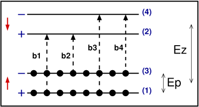
Figure 2: (color online) Schematic representation of the four highly degenerate lowest Landau levels when $E_{Z}>E_{P}$. The state $|{\rm SFM}\rangle$ is obtained by completely filling the energy levels (1) and (3). b1, b2, b3, and b4 are the elementary neutral excitations which are related to the density operators $\rho_{21}({\bf q})$, $\rho_{23}({\bf q})$, $\rho_{41}({\bf q})$, and $\rho_{43}({\bf q})$ respectively.

The commutation relations between $\rho_{IJ}({\bf q})$ ($I=1,3$ and $J=2,4$) and their respective Hermitian conjugates $\rho_{JI}(-{\bf q})$ read [see Eq. (8)]

$$[\rho_{IJ}({\bf q}),\rho_{JI}({\bf q}^{\prime})] = e^{{\bf q}\cdot{\bf q}^{\prime}l^{2}/2}\left[e^{i{\bf q}\wedge{\bf q}^{\prime}/2}\rho_{II}({\bf q}+{\bf q}^{\prime})\right.$$ (32)

$$-\left.e^{-i{\bf q}\wedge{\bf q}^{\prime}/2}\rho_{JJ}({\bf q}+{\bf q}^{\prime})\right].$$

Here, the expansions of $\rho_{11}({\bf q})$, $\rho_{22}({\bf q})$, $\rho_{33}({\bf q})$, and $\rho_{44}({\bf q})$ around the reference state $|{\rm SFM}\rangle$ are given by

$$\rho_{II}({\bf q}) = \langle{\rm SFM}|\rho_{II}({\bf q})|{\rm SFM}\rangle+\delta\rho_{II}({\bf q})$$ (33)

$$= {\rm N_{\phi}}(\delta_{I,1}+\delta_{I,3})\delta_{{\bf q},0}+\delta\rho_{II}({\bf q}),$$

and therefore the commutation relations (32) reduce to (neglecting the density fluctuations $\delta\rho_{II}({\bf q})$)

$$[\rho_{IJ}({\bf q}),\rho_{JI}({\bf q}^{\prime})]\approx\delta_{{\bf q},-{\bf k}}{\rm N_{\phi}}e^{(ql)^{2}/2}.$$

Using the same arguments of the previous section, we assume that $\rho_{21}({\bf q})$, $\rho_{41}({\bf q})$, $\rho_{23}({\bf q})$, and $\rho_{43}({\bf q})$ are approximately boson operators. Indeed, they are independent operators because

$$\rho_{IJ}({\bf q}) = \langle{\rm SFM}|\rho_{IJ}({\bf q})|{\rm SFM}\rangle+\delta\rho_{IJ}({\bf q})\approx 0,$$ (34)

for $(I,J)=(1,3)$ and $(4,2)$.

To sum up, the spin phase is characterized by a set of four independent boson operators defined as

$$b^{\dagger}_{1}({\bf q}) \equiv \alpha_{q}\rho_{21}({\bf q}),\;\;\;\;\;\;b_{1}({\bf q})\equiv\alpha_{q}\rho_{12}(-{\bf q}),$$

$$b^{\dagger}_{2}({\bf q}) \equiv \alpha_{q}\rho_{23}({\bf q}),\;\;\;\;\;\;b_{2}({\bf q})\equiv\alpha_{q}\rho_{32}(-{\bf q}),$$

$$b^{\dagger}_{3}({\bf q}) \equiv \alpha_{q}\rho_{41}({\bf q}),\;\;\;\;\;\;b_{3}({\bf q})\equiv\alpha_{q}\rho_{14}(-{\bf q}),$$ (35)

$$b^{\dagger}_{4}({\bf q}) \equiv \alpha_{q}\rho_{43}({\bf q}),\;\;\;\;\;\;b_{4}({\bf q})\equiv\alpha_{q}\rho_{34}(-{\bf q}),$$

with $\alpha_{q}=e^{(lq)^{2}/4}/\sqrt{{\rm N_{\phi}}}$, and obeying the canonical boson algebra (25).

The introduction of new boson operators implies that the expansions of the density operators $\rho_{II}({\bf q})$ in terms of the bosons are no longer given by Eqs. (26) and (27). Following the same procedure discussed in the previous section, it is possible to show that

$$\rho_{11}({\bf q}) = {\rm N_{\phi}}\delta_{{\bf q},0}-\sum_{{\bf k}\;i=1,3}e^{-(lq)^{2}/4-i{\bf q}\wedge{\bf k}/2}b^{\dagger}_{i}({\bf q}+{\bf k})b_{i}({\bf k}),$$

$$\rho_{22}({\bf q}) = \sum_{{\bf k}\;i=1,2}e^{-(lq)^{2}/4+i{\bf q}\wedge{\bf k}/2}b^{\dagger}_{i}({\bf q}+{\bf k})b_{i}({\bf k}),$$

$$\rho_{33}({\bf q}) = {\rm N_{\phi}}\delta_{{\bf q},0}-\sum_{{\bf k}\;i=2,4}e^{-(lq)^{2}/4-i{\bf q}\wedge{\bf k}/2}b^{\dagger}_{i}({\bf q}+{\bf k})b_{i}({\bf k}),$$

$$\rho_{44}({\bf q}) = \sum_{{\bf k}\;i=3,4}e^{-(lq)^{2}/4+i{\bf q}\wedge{\bf k}/2}b^{\dagger}_{i}({\bf q}+{\bf k})b_{i}({\bf k}).$$ (36)

By adding up the four terms above, one can see that the electron density operator $\rho({\bf q})$ [Eq. (12)] also has the form (28) with the replacements $\sum_{i=1}^{3}\rightarrow\sum_{i=1}^{4}$ and ${\rm N_{\phi}}\delta_{{\bf q},0}\rightarrow 2{\rm N_{\phi}}\delta_{{\bf q},0}$. However, the boson representation of the z-components of the spin and pseudospin density operators and the mixed operator $P_{Z}S_{Z}({\bf q})$ are modified, i.e.,

$$S_{Z}({\bf q}) = {\rm N_{\phi}}\delta_{{\bf q},0}-e^{-(lq)^{2}/4}$$ (37)

$$\times\sum_{i,{\bf k}}\cos\left({\bf q}\wedge{\bf k}/2\right)b^{\dagger}_{i}({\bf q}+{\bf k})b_{i}({\bf k}),$$

$$I^{\mu}_{Z}({\bf q}) = \sum_{i,{\bf k}}f^{\mu}_{i}({\bf q},{\bf k})b^{\dagger}_{i}({\bf q}+{\bf k})b_{i}({\bf k}),$$ (38)

where $\sum_{i}=\sum_{i=1}^{4}$, $I^{\mu}_{Z}({\bf q})=P_{\rm Z}({\bf q})$ and $S_{\rm Z}P_{\rm Z}({\bf q})$, and the form factors are given by

$$f^{P}_{1}({\bf q},{\bf k}) = -f^{P}_{4}({\bf q},{\bf k})=ie^{-(lq)^{2}/4}\sin\left({\bf q}\wedge{\bf k}\right/2),$$

$$f^{P}_{2}({\bf q},{\bf k}) = -f^{P}_{3}({\bf q},{\bf k})=e^{-(lq)^{2}/4}\cos\left({\bf q}\wedge{\bf k}\right/2),$$ (39)

and

$$f^{PS}_{1}({\bf q},{\bf k}) = -f^{PS}_{4}({\bf q},{\bf k})=-e^{-(lq)^{2}/4}\cos\left({\bf q}\wedge{\bf k}\right/2),$$

$$f^{PS}_{2}({\bf q},{\bf k}) = -f^{PS}_{3}({\bf q},{\bf k})=-ie^{-(lq)^{2}/4}\sin\left({\bf q}\wedge{\bf k}\right/2).$$

Finally, the new bosonic expressions of $\rho_{12}({\bf q})$, $\rho_{21}({\bf q})$, $\rho_{34}({\bf q})$, and $\rho_{43}({\bf q})$ are shown in the Appendix B [see Eqs. (LABEL:ops1-sfm) and (LABEL:ops2-sfm)].

II.4 Pseudospin phase

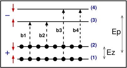
Figure 3: (color online) Schematic representation of the four highly degenerate lowest Landau levels when $E_{Z}<E_{P}$. The state $|{\rm PFM}\rangle$ is obtained by completely filling the energy levels (1) and (2). b1, b2, b3, and b4 are the elementary neutral excitations which are related to the density operators $\rho_{31}({\bf q})$, $\rho_{32}({\bf q})$, $\rho_{41}({\bf q})$, and $\rho_{42}({\bf q})$ respectively.

The situation here is quite similar to the one discussed in the previous section, because again ${\rm N}=2{\rm N_{\phi}}$ but now $E_{Z}<E_{P}$. As a consequence, the ground state of the noninteracting model (3) is a spin-singlet pseudospin-polarized state,

$$|{\rm PFM}\rangle=\prod_{m=1}^{{\rm N_{\phi}}-1}c^{\dagger}_{m\,+\,\downarrow}c^{\dagger}_{m\,+\,\uparrow}|0\rangle,$$ (40)

and the elementary neutral excitations are now related to $\rho_{31}({\bf q})$, $\rho_{32}({\bf q})$, $\rho_{41}({\bf q})$, and $\rho_{42}({\bf q})$ [see Fig. 3].

Again, one can show that the above four density operators give rise to four independent boson operators, i.e.,

$$b^{\dagger}_{1}({\bf q}) \equiv \alpha_{q}\rho_{31}({\bf q}),\;\;\;\;\;\;b_{1}({\bf q})\equiv\alpha_{q}\rho_{13}(-{\bf q}),$$

$$b^{\dagger}_{2}({\bf q}) \equiv \alpha_{q}\rho_{32}({\bf q}),\;\;\;\;\;\;b_{2}({\bf q})\equiv\alpha_{q}\rho_{23}(-{\bf q}),$$

$$b^{\dagger}_{3}({\bf q}) \equiv \alpha_{q}\rho_{41}({\bf q}),\;\;\;\;\;\;b_{3}({\bf q})\equiv\alpha_{q}\rho_{14}(-{\bf q}),$$ (41)

$$b^{\dagger}_{4}({\bf q}) \equiv \alpha_{q}\rho_{42}({\bf q}),\;\;\;\;\;\;b_{4}({\bf q})\equiv\alpha_{q}\rho_{24}(-{\bf q}),$$

which satisfy the boson algebra (25). Indeed, the commutator of each density operator with its corresponding Hermitian conjugate is also given by Eq. (32) with $I=1,2$ and $J=3,4$. The expansion (33) is replaced by

$$\rho_{II}({\bf q}) = \langle{\rm PFM}|\rho_{II}({\bf q})|{\rm PFM}\rangle+\delta\rho_{II}({\bf q})$$ (42)

$$= {\rm N_{\phi}}(\delta_{I,1}+\delta_{I,2})\delta_{{\bf q},0}+\delta\rho_{II}({\bf q}),$$

while Eq. (34) is preserved, but now $(I,J)=(1,2)$ and $(4,3)$.

The set of creation and annihilation boson operators (41) implies that Eqs. (36) should be replaced by

$$\rho_{11}({\bf q}) = {\rm N_{\phi}}\delta_{{\bf q},0}-\sum_{{\bf k},i=1,3}e^{-(lq)^{2}/4-i{\bf q}\wedge{\bf k}/2}b^{\dagger}_{i}({\bf q}+{\bf k})b_{i}({\bf k}),$$

$$\rho_{22}({\bf q}) = {\rm N_{\phi}}\delta_{{\bf q},0}-\sum_{{\bf k},i=2,4}e^{-(lq)^{2}/4-i{\bf q}\wedge{\bf k}/2}b^{\dagger}_{i}({\bf q}+{\bf k})b_{i}({\bf k}),$$

$$\rho_{33}({\bf q}) = \sum_{{\bf k},i=1,2}e^{-(lq)^{2}/4+i{\bf q}\wedge{\bf k}/2}b^{\dagger}_{i}({\bf q}+{\bf k})b_{i}({\bf k}),$$

$$\rho_{44}({\bf q}) = \sum_{{\bf k},i=3,4}e^{-(lq)^{2}/4+i{\bf q}\wedge{\bf k}/2}b^{\dagger}_{i}({\bf q}+{\bf k})b_{i}({\bf k}).$$ (43)

Again, the expression (28) for the electron density operator is preserved, apart from the changes $\sum_{i=1}^{3}\rightarrow\sum_{i=1}^{4}$ and ${\rm N_{\phi}}\delta_{{\bf q},0}\rightarrow 2{\rm N_{\phi}}\delta_{{\bf q},0}$. When compared with the results of Sec. II.3, the boson representation of the $z$-components of the spin, pseudospin, and mixed spin-pseudospin density operators are interchanged, i.e.,

$$I^{\mu}_{Z}({\bf q}) = \sum_{i,{\bf k}}f^{\mu}_{i}({\bf q},{\bf k})b^{\dagger}_{i}({\bf q}+{\bf k})b_{i}({\bf k}),$$ (44)

$$P_{Z}({\bf q}) = {\rm N_{\phi}}\delta_{{\bf q},0}-e^{-(lq)^{2}/4}$$ (45)

$$\times\sum_{i,{\bf k}}\cos\left({\bf q}\wedge{\bf k}/2\right)b^{\dagger}_{i}({\bf q}+{\bf k})b_{i}({\bf k}),$$

with $I^{\mu}_{Z}({\bf q})=S_{Z}({\bf q})$ and $P_{Z}S_{Z}({\bf q})$, and

$$f^{S}_{1}({\bf q},{\bf k}) = -f^{S}_{4}({\bf q},{\bf k})=ie^{-(lq)^{2}/4}\sin\left({\bf q}\wedge{\bf k}\right/2),$$

$$f^{S}_{2}({\bf q},{\bf k}) = -f^{S}_{3}({\bf q},{\bf k})=e^{-(lq)^{2}/4}\cos\left({\bf q}\wedge{\bf k}\right/2),$$

and

$$f^{PS}_{1}({\bf q},{\bf k}) = -f^{PS}_{4}({\bf q},{\bf k})=-e^{-(lq)^{2}/4}\cos\left({\bf q}\wedge{\bf k}\right/2),$$

$$f^{PS}_{2}({\bf q},{\bf k}) = -f^{PS}_{3}({\bf q},{\bf k})=-ie^{-(lq)^{2}/4}\sin\left({\bf q}\wedge{\bf k}\right/2).$$

We again refer the reader to the Appendix B for the boson representation of the operators $\rho_{12}({\bf q})$, $\rho_{21}({\bf q})$, $\rho_{34}({\bf q})$, and $\rho_{43}({\bf q})$.

The generalization of the bosonization methoddoretto for the case of electrons restricted to the lowest Landau level and in the presence of two discrete degrees of freedom is concluded. The next sections will be devoted to an application of the formalism.

III Quantum Hall ferromagnetism in graphene

In this section, we apply the methodology developed above to study the QHE at $\nu=\pm 1$ and $\nu=0$ in graphene. We will follow the lines of Ref. doretto, and derive an effective boson model for the system. Our starting point is the continuous model for graphene recently proposed by Alicea and Fisher.alicea06 Before outlining the derivation of this model, we will briefly review some aspects of the Landau level spectrum in graphene.

III.1 Preliminaries on graphene

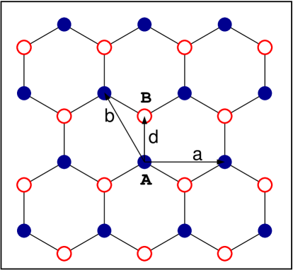
Figure 4: (color online) Schematic representation of the honeycomb lattice. The triangular sublattices A and B are respectively represented by blue and red circles. $\mathbf{a}$ and $\mathbf{b}$ are the primitive vectors of the underline triangular sublattice A and $\mathbf{d}$ is the basis vector.

Graphene is a collection of carbon atoms, which are arranged in a two-dimensional honeycomb lattice, as it is illustrated in Fig. 4.castroneto06 ; ando The lattice structure is triangular with two atoms per unit cell located at the positions $(0,0)$ and $\mathbf{d}=a_{0}(0,1/\sqrt{3})$. The lattice spacing is $a_{0}=2.46\;\AA$. It might also be seem as two interpenetrating triangular sublattices A and B. The primitive vectors of the (A) triangular lattice are $\mathbf{a}=a_{0}(1,0)$ and $\mathbf{b}=a_{0}(-1/2,\sqrt{3}/2)$, and therefore the primitive vectors of the reciprocal lattice are $\mathbf{a}^{*}=(2\pi/a_{0})(1,1/\sqrt{3})$ and $\mathbf{b}^{*}=(2\pi/a_{0})(0,2/\sqrt{3})$. In this atomic arrangement, the carbon atoms are connected by strong covalent $\sigma$-bonds, derived from the $sp^{2}$ hybridization of the atomic orbitals. The remaining $p_{z}$ orbitals (perpendicular to the plane) have a weak overlap and therefore they form a narrow band of $\pi$-orbitals, through which the Fermi level passes.altland By describing the $\pi$-electrons within a tight-binding model

$$\mathcal{H}_{t}=-t\sum_{\langle i,j\rangle}\sum_{\sigma=\uparrow,\downarrow}\left(a^{\dagger}_{i,\sigma}b_{j\sigma}+h.c.\right),$$ (46)

where $t\approx 2.7\,eV$ is the nearest-neighbor hopping energy and the operators $a^{\dagger}_{i,\sigma}$ and $b^{\dagger}_{i,\sigma}$ create a spin $\sigma$ electron on site $i$ of the sublattices A and B respectively, one can show that the single-particle electron energy varies linearly with momentum ($\epsilon_{q}=\pm\hbar v_{F}|{\bf q}|$, with $v_{F}=a_{0}\sqrt{3}t/2\approx 10^{6}\,m/s$) around the six corners of the (hexagonal) Brillouin zone, i.e., the band structure consists of six Dirac cones. Only two of them are inequivalent, and here we consider the ones around the points $\mathbf{K}=(2\pi/a_{0})(2/3,0)$ and $\mathbf{K}^{\prime}=-(2\pi/a_{0})(2/3,0)$. In the undoped case, there is only one $\pi$-electron per carbon atom, the Fermi level lies at the Dirac points and therefore the system is semi-metallic. By using a gate-voltage, it is possible to modify the carriers, either $p$-type or $n$-type (doped case).

The fact that the electronic structure of the system may be described by an effective massless (continuous) Dirac model has some important consequences. In particular, when a perpendicular magnetic field is applied, a different Landau level structure emerges when compared to the Schrödinger-like one observed in the two-dimensional electron gas in GaAs heterostructures. Indeed, one can show that the energy of the (Dirac) Landau levels are given by

$$E_{n,\sigma}=\mp\frac{1}{2}E_{Z}+{\rm sign(n)}\sqrt{2\hbar v^{2}_{F}B|n|/c},$$ (47)

respectively for $\sigma=\,\uparrow$ and $\downarrow$, which are associated with the two-components spinor eigenvectors ($n\not=0$)

$$|\hat{\Phi}_{n,m,\sigma,\alpha=+}\rangle = \frac{1}{\sqrt{2}}\left(\begin{array}[]{c}|n\,m\rangle\\ {\rm sign(n)}|n-1\,m\rangle\end{array}\right),$$ (50)

$$|\hat{\Phi}_{n,m,\sigma,\alpha=-}\rangle = \frac{1}{\sqrt{2}}\left(\begin{array}[]{c}{\rm sign(n)}|n-1\,m\rangle\\ |n\,m\rangle\end{array}\right).$$ (54)

For $n=0$, we have

$$|\hat{\Phi}_{0,m,\sigma,+}\rangle=\left(\begin{array}[]{c}|0\,m\rangle\\ 0\end{array}\right)\;\;\;\;{\rm and}\;\;\;\;|\hat{\Phi}_{0,m,\sigma,-}\rangle=\left(\begin{array}[]{c}0\\ |0\,m\rangle\end{array}\right).$$ (55)

Here, $\alpha=\pm$ corresponds, respectively, to $\mathbf{K}$ and $\mathbf{K}^{\prime}$ points, $m$ is the guiding center quantum number, and $|n\,m\rangle$ are the Schrödinger’s Landau level eigenvectors. Each spinor component is related to one of the triangular sublattices A and B. For $n\not=0$, each eigenvector $|\hat{\Phi}_{n,m,\sigma,+}\rangle$ and $|\hat{\Phi}_{n,m,\sigma,-}\rangle$ has a weight (probability) equally distributed between the two sublattices, while the lowest Landau level eigenvectors $|\hat{\Phi}_{0,m,\sigma,+}\rangle$ and $|\hat{\Phi}_{0,m,\sigma,-}\rangle$ are respectively localized on sublattices A and B. The results (47)-(55) show that the Dirac Landau levels are approximately four-fold degenerate due to the electronic spin and valley ($\alpha=\pm$) degrees of freedom.

Let us concentrate on the integer quantum Hall states in the lowest Landau level ($n=0$). Apart from the fact that the fermion field operator $\hat{\Psi}({\bf r})$ is a two-component spinor and the momenta ${\bf q}$ are measured with respect to the ${\bf K}$ and ${\bf K}^{\prime}$ points [we refer the reader for a detailed discussion in the Appendix C], the methodology developed in the previous section can be used to study the QHE at $\nu=-1$ and $\nu=0$. In fact, the former, which corresponds to a quarter filled lowest Landau level, is associate with the spin-pseudospin polarized phase (Sec. II.2), whereas the latter, characterize by a half filled lowest Landau level, is associate with either the spin (Sec. II.3) or the pseudospin (Sec. II.4) phases.

III.2 Alicea and Fisher’s model

The effective continuous model proposed by Alicea and Fisher to study the quantum Hall effect in graphene goes beyond the tight-binding approximation [see Ref. alicea06, for details]. In addition to $\mathcal{H}_{t}$ [Eq.(46)], it also includes the on-site electron-electron repulsion term $\mathcal{H}_{U}$ and the (long range) Coulomb interaction $\mathcal{H_{\rm Coul}}$, namely

$$\mathcal{H}=\mathcal{H}_{t}+\mathcal{H}_{U}+\mathcal{H_{\rm Coul}},$$ (56)

where

$$\mathcal{H}_{U}=U\sum_{i}\left[\frac{1}{4}(\hat{n}_{i})^{2}-\frac{1}{3}\mathbf{S}_{i}\cdot\mathbf{S}_{i}\right]$$ (57)

and

$$\mathcal{H_{\rm Coul}}=\frac{1}{2}\sum_{i\not=j}V({\bf r}_{i}-{\bf r}_{j})\hat{n}_{i}\hat{n}_{j}.$$ (58)

Here, $U$ is the on-site repulsion energy and $V(r)=e^{2}/\epsilon r$ is the Coulomb potential, with an estimated dielectric constant $\epsilon\approx 5$ [the energy scales for graphene are listed in the Appendix A]. The electron number operator is $\hat{n}_{i}=c^{\dagger}_{i,\uparrow}c_{i\uparrow}+c^{\dagger}_{i,\downarrow}c_{i\downarrow}$, $\mathbf{S}_{i}=(1/2)\sum_{\sigma,\lambda}c^{\dagger}_{i,\sigma}\hat{\sigma}_{\sigma\lambda}c_{i\lambda}$, is the spin operator, where $\hat{\sigma}$ is a vector of Pauli matrices, and $c^{\dagger}_{i,\sigma}=a^{\dagger}_{i,\sigma}$ or $b^{\dagger}_{i,\sigma}$ depending whether $i$ is on sublattice A or B.

Starting from the Hamiltonian (56), a continuous interacting theory was derived by expanding the fermion operators $a^{\dagger}_{i,\sigma}$ and $b^{\dagger}_{i,\sigma}$ around the two Dirac points $\mathbf{K}$ and $\mathbf{K}^{\prime}$. After adding a perpendicular magnetic field $\mathbf{B}=B\hat{z}$ and projecting into the lowest Landau level, the model may be rewritten as

$$\mathcal{H}=\mathcal{H}_{SU4}+\mathcal{H}_{SB}$$ (59)

where

$$\mathcal{H}_{SU4}=\frac{1}{2}\sum_{\bf q}v(q)\rho({\bf q})\rho(-{\bf q})$$ (60)

is the SU(4) invariant part of the Hamiltonian, with $v(q)=2\pi e^{2}/\epsilon q$ (the Fourier transform of the Coulomb potential in two-dimensions), andnota

$$\mathcal{H}_{SB} = -E_{Z}S_{\rm Z}({\bf q}=0)-4\sum_{\bf q}v_{1}({\bf q})P_{\rm Z}({\bf q})P_{\rm Z}(-{\bf q})$$ (61)

$$+u_{0}\sum_{\bf q}\left[\frac{1}{4}\rho({\bf q})\rho(-{\bf q})+P_{\rm Z}({\bf q})P_{\rm Z}(-{\bf q})\right.$$

$$\left.-\frac{1}{3}\mathbf{S}({\bf q})\cdot\mathbf{S}(-{\bf q})-\frac{1}{3}P_{\rm Z}\mathbf{S}({\bf q})\cdot P_{\rm Z}\mathbf{S}(-{\bf q})\right]$$

contains terms that break the SU(4) symmetry. The parameter $u_{0}$ is related to the on-site repulsion energy [$u_{0}=\sqrt{3}a_{0}^{2}U/4$] and $v_{1}({\bf q})$ is the Fourier transform of

$$v_{1}({\bf r})=\frac{\sqrt{3}a_{0}^{2}}{8}\left[V(r+\hat{y}/\sqrt{3})-\left(1-\delta_{{\bf r},0}\right)V(r)\right].$$ (62)

The model (59) was analyzed in two distinct situations: (i) the quantum Hall ferromagnetic regime, which corresponds to an ideal, completely clean sample, and (ii) the quantum Hall paramagnetic regime, where disorder effects are very strong (very dirty sample). Here, we will only focus on the quantum Hall ferromagnetic regime. The interplay between disorder and electron-electron interactions will be postponed for a future publication.

In order to derive an effective boson model for the quantum Hall states at $\nu=-1$ and $\nu=0$, we just need to substitute the respective boson representation of the electron density, the spin, pseudospin and mixed spin-pseudospin density operators into the Hamiltonian (59) and normal order the resulting expression. Although the expansion of the electron density operator is similar for the three phases, each quantum Hall state should be treated separately because the expansions in terms of bosons of the spin/pseudospin density operators vary from phase to phase.

III.2.1 Filling factor $\nu=-1$

We start by considering the QHE at $\nu=-1$. The state at $\nu=+1$ is related to it by particle-hole symmetry and will not be discussed here.

SU(4) invariant terms - Let us firstly analyzed the SU(4) invariant part of the Hamiltonian (59). Substituting the boson representation of the electron density operator [Eq.(28)] in $\mathcal{H}_{SU4}$ [Eq.(60)] and normal ordering the boson operators, apart from a constant related to the positive background, we arrive at the following interacting boson model

$$\mathcal{H}_{SU4}^{B}=\mathcal{H}_{0}^{B}+\mathcal{H}_{I}^{B},$$ (63)

where the quadratic part is given by

$$\mathcal{H}_{0}^{B}=\sum_{i=1}^{3}\sum_{\bf q}w_{q}b^{\dagger}_{i}({\bf q})b_{i}({\bf q})$$ (64)

and the quartic term reads

$$\mathcal{H}_{I}^{B}=\sum_{i,j=1}^{3}\sum_{{\bf q},{\bf p},{\bf k}}v_{\bf q}({\bf k},{\bf p})b^{\dagger}_{i}({\bf k}+{\bf q})b^{\dagger}_{j}({\bf p}-{\bf q})b_{j}({\bf p})b_{i}({\bf k}).$$ (65)

The effective boson model (63) is the SU(4) counterpart of the boson model derived in Ref. doretto, for the two-dimensional electron gas at $\nu=1$ realized in GaAs heterostructures (hereafter called 2DEG at $\nu=1$). The ground state of the model (63) is the boson vacuum, which is the spin-pseudospin polarized state $|{\rm SPFM}\rangle$. Notice that this state is indeed a spin polarized charge density wave (CDW) because the electronic distribution is concentrated only in one sublattice [see Eqs. (55) and the discussion below this equation]. $\mathcal{H}^{B}_{0}$ describes three well-defined branches of bosonic excitations, characterized by the same dispersion relation

$$w_{q}=\frac{e^{2}}{\epsilon l}\sqrt{\frac{\pi}{2}}\left[1-e^{-(lq)^{2}/4}I_{0}\left((lq)^{2}/4\right)\right],$$ (66)

where $I_{0}(x)$ is the modified Bessel function of the first kind.arfken Eq. (66) is equal to the dispersion relation of the elementary neutral excitations (magnetic excitons) of the 2DEG at $\nu=1$.doretto ; kallin In the long wavelength limit, $w_{q}\approx\epsilon_{B}|l{\bf q}|^{2}$ with $\epsilon_{B}=\sqrt{\pi/32}\;(e^{2}/\epsilon l)$, and therefore the branch $i=1$ corresponds to spin wave excitations, while the branches $i=2$ and $i=3$ to pseudospin wave and mixed spin-pseudospin wave excitations, respectively [see Fig. 1]. At short wavelengths $w_{q}\approx\sqrt{\pi/2}\;(e^{2}/\epsilon l)$, which is the energy of a very-well separated particle-hole pair.kallin Finally, the boson-boson interaction potential is given by

$$v_{\bf q}({\bf k},{\bf p})=2v(q)e^{-(lq)^{2}/2}\sin\left({\bf q}\wedge{\bf k}\right/2)\sin\left({\bf q}\wedge{\bf p}\right/2).$$ (67)

Apart from the fact that Eq. (65) describes scattering processes between bosons within the same ($i=j$) and different ($i\not=j$) branches, the interaction potential (67) is similar to the one derived in Ref. doretto, . It is worth mentioning that our approach also provides an interaction between the bosonic excitations, which is not captured by the analysis presented in Ref. alicea06, .

Due to the similarities between the quantum Hall system in graphene at $\nu=-1$ and the 2DEG at $\nu=1$, we would expect that the charged excitations of the former might be described by topological solitonssondhi ; sondhi99 (quantum Hall skyrmions) as well. In fact, the situation here is formally identical to the one in the (spinfull) bilayer QHS at $\nu_{T}=1$ in GaAs heterostructures. The similarity clearly appears when the upper-layer and down-layer electronic states are combined into the bounding and anti-bounding states. In this case, there are four possible kinds of charged excitations with topological charge $Q_{T}=\pm 1$ (and corresponding electric charge $Q_{e}=eQ_{T}$), namely one skyrmion ($Q_{T}=1$ and $Q_{e}=e$) and three types of antiskyrmions ($Q_{T}=-1$ and $Q_{e}=-e$). Indeed, they might be considered as SU(4) skyrmions because the topological excitation created by introducing an extra electric charge should involve the three branches of neutral excitations in order to minimize the total energy [see Ref.  ezawa04, for a detailed description of SU(4) skyrmions in the context of the bilayers].

For the SU(2) version of the model (63), we know that the boson-boson interaction potential (67) gives rise to bound states of two-bosons which are related to small [SU(2)] skyrmion-antiskyrmion pair excitations.doretto The fact that (67) describes scattering processes between different bosonic branches indicates that here we would expect bound states constituted by bosons belonging to the same and distinct branches. Moreover, it was also shown that by describing the topological excitation as a coherent state of bosons $|{\rm sk}\rangle$ [see Eq. (64) of Ref. doretto, ], the expectation value of the SU(2) boson model with respect to the state $|{\rm sk}\rangle$ is equal to the energy functional derived from the phenomenological theory of Sondhi et al.sondhi for the quantum Hall skyrmion, i.e., the semiclassical limit of the SU(2) boson model agrees with Sondhi’s theory for the quantum Hall skyrmion.

It is quite straightforward to derive the semiclassical limit of the interacting boson model (63). We start by writing down the SU(4) counterpart of the state $|{\rm sk}\rangle$,

$$|{\rm sk}\rangle=\exp\left(\mathcal{B}\sum_{i=1}^{3}\sum_{{\bf q}}\Omega^{i}_{\bf q}b^{\dagger}_{i}(-{\bf q})+\bar{\Omega}^{i}_{\bf q}b_{i}({\bf q})\right)|{\rm SPFM}\rangle,$$ (68)

where $(\bar{\Omega}^{i}_{-{\bf q}})^{*}=\Omega^{i}_{\bf q}$ and the constant $\mathcal{B}$ will be determined latter. With the aid of the Baker-Hausdorff formula, one can show that the expectation value in the state $|{\rm sk}\rangle$ of normal ordered boson operators is obtained just by replacing each $b^{\dagger}_{i}({\bf q})$ and $b_{i}({\bf q})$ respectively for $i\mathcal{B}\bar{\Omega}^{i}_{\bf q}$ and $-i\mathcal{B}\Omega^{i}_{-{\bf q}}$. Defining the excess charge $\delta\rho({\bf q})=\langle sk|\rho({\bf q})|sk\rangle-{\rm N_{\phi}}\delta_{{\bf q},0}$, where $\rho({\bf q})$ is the electron density operator (28), we have

$$\delta\rho({\bf q})=2i\sum_{i=1}^{3}\sum_{\bf k}e^{-(lq)^{2}/2}\sin\left({\bf q}\wedge{\bf k}/2\right)\bar{\Omega}^{i}_{{\bf k}+{\bf q}}\Omega^{i}_{\bf k}.$$ (69)

Assuming that the Fourier transform of $\bar{\Omega}^{i}_{\bf q}$ and $\Omega^{i}_{\bf q}$ vary slowly in space, we can restrict ourselves to the long wavelength limit of Eq. (69), i.e., we can consider $e^{-(lq)^{2}/2}\sin\left({\bf q}\wedge{\bf k}/2\right)\approx{\bf q}\wedge{\bf k}/2$. Within this approximation, the Fourier transform of $\delta\rho({\bf q})$ is given by

$$\delta\rho({\bf r})=i\mathcal{B}^{2}l^{2}\sum_{i}\hat{z}\cdot\nabla\bar{\Omega}^{i}({\bf r})\times\nabla\Omega^{i}({\bf r}),$$ (70)

which is in agreement with the expression for the topological charge density derived by Arovas et al.arovas99 in their studies of SU(N) quantum Hall skyrmions. Indeed, by comparing Eq. (70) with Eq. (3) from Ref. arovas99, , one concludes that $\mathcal{B}=1/\sqrt{2\pi l^{2}}$. Once the constant $\mathcal{B}$ is fixed, we can now calculate $\langle sk|\mathcal{H}^{B}_{SU4}|sk\rangle$ and show that

$$\langle\mathcal{H}^{B}_{SU4}\rangle = 2\rho^{0}_{S}\sum_{i}\int\;d^{2}r|\nabla\Omega^{i}({\bf r})|^{2}$$ (71)

$$+ \frac{1}{2}\int\;d^{2}rd^{2}r^{\prime}v\left(|{\bf r}-{\bf r}^{\prime}|\right)\delta\rho({\bf r})\delta\rho({\bf r}^{\prime}),\;\;\;\;$$

where $\rho^{0}_{S}=1/(16\sqrt{2\pi})\;e^{2}/\epsilon l$ is the stiffness and $v(r)=e^{2}/\epsilon r$ is the Coulomb potential. The energy functional $E[\Omega^{i}({\bf r})]=\langle\mathcal{H}^{B}_{SU4}\rangle$ [Eq. (71)], which corresponds to the SU(4) counterpart of Sondhi’s model, agrees with the findings of Arovas and co-workers.arovas99 This analysis shows that the boson model (63) can indeed be used to study SU(4) quantum Hall skyrmions in graphene.

Symmetry breaking terms - The degeneracy of the three branches of boson excitations is lifted when the SU(4) symmetry breaking term $\mathcal{H_{SB}}$ is taken into account. Following the same procedure used above, we can derive an effective boson model from the Hamiltonian (61). The task here is slightly more difficult because $\mathcal{H_{SB}}$ involves more complex expressions.

Let us start by expanding the operators $\mathbf{S}({\bf q})$ and $P_{\rm Z}\mathbf{S}({\bf q})$ in terms of the density operators $\rho_{IJ}({\bf q})$. It is possible to show that

$$\mathbf{S}({\bf q})\cdot\mathbf{S}(-{\bf q}) + P_{\rm Z}\mathbf{S}({\bf q})\cdot P_{\rm Z}\mathbf{S}(-{\bf q})=$$

$$S_{\rm Z}({\bf q})S_{\rm Z}(-{\bf q}) + P_{\rm Z}S_{\rm Z}({\bf q})P_{\rm Z}S_{\rm Z}(-{\bf q})+\rho_{12}({\bf q})\rho_{21}(-{\bf q})$$

$$+\,\rho_{21}({\bf q})\rho_{12}(-{\bf q}) + \rho_{34}({\bf q})\rho_{43}(-{\bf q})+\rho_{43}({\bf q})\rho_{34}(-{\bf q}).$$

The boson representations of the above density operators $\rho_{IJ}({\bf q})$ are shown in the Appendix B [see Eqs. (LABEL:ops1-spfm) and (92)]. After a lengthy but straightforward calculation, one can show that $\mathcal{H}_{SB}$ is also mapped into an interacting boson model. Adding Eq. (63), which was derived from the SU(4) invariant term, the total effective boson model may be written as

$$\mathcal{H}^{B}=\bar{\mathcal{H}}_{0}^{B}+\bar{\mathcal{H}}_{I}^{B}.$$ (72)

The quadratic term now reads

$$\bar{\mathcal{H}}_{0}^{B}=\sum_{i=1}^{3}\sum_{\bf q}\bar{\omega}_{i}({\bf q})b^{\dagger}_{i}({\bf q})b_{i}({\bf q}),$$ (73)

where $\bar{\omega}_{i}(q)$ are the renormalized boson dispersion relations,

$$\bar{\omega}_{1}(q) = E_{Z}+2(u_{0}-u_{1}){\rm N_{\phi}}\left(1-e^{-(lq)^{2}/2}\right)+w_{q},$$

$$\bar{\omega}_{2}(q) = 4u_{1}{\rm N_{\phi}}-4\sum_{\bf k}v_{1}({\bf k})e^{-(lk)^{2}/2}$$

$$\times\cos^{2}\left({\bf k}\wedge{\bf q}/2\right)+w_{q},$$

$$\bar{\omega}_{3}(q) = E_{Z}+\bar{\omega}_{2}(q),$$ (74)

with $w_{q}$ given by Eq. (66) and $u_{1}=v_{1}({\bf q}=0)$ [see Eq. (62)]. In the small momentum region, we have

$$\bar{\omega}_{1}(q)\approx\Delta_{i}+4\pi\rho^{i}_{S}|l{\bf q}|^{2},$$ (75)

where the excitation gaps $\Delta_{i}$ and the renormalized stiffnesses are given by

$$\Delta_{1} = E_{Z},\;\;\;\;\;\;\;\;\;\;\;\;\Delta_{2}=\sqrt{\pi^{3}/24}(a_{0}/l)u_{1}{\rm N_{\phi}},$$

$$\Delta_{3} = \Delta_{1}+\Delta_{2},$$

$$\rho^{1}_{S} = {\rm N_{\phi}}(u_{0}-u_{1})/4\pi+\rho^{0}_{S},\;\;\;\;\;\;$$

$$\rho^{2}_{S} = \rho^{3}_{S}=u_{1}{\rm N_{\phi}}/4\pi+\rho^{0}_{S}.$$ (76)

Notice that $\bar{\omega}_{2}(q=0)\ll\bar{\omega}_{1}(q=0)$ and $\bar{\omega}_{3}(q=0)$. Both small and large momentum limits of Eqs. (74) agree with the results derived by Alicea and Fisher.alicea06 The interaction term assumes the form

$$\bar{\mathcal{H}}_{I}^{B}=\sum_{i,j=1}^{3}\sum_{{\bf q},{\bf p},{\bf k}}\bar{v}^{i,j}_{\bf q}({\bf k},{\bf p})b^{\dagger}_{i}({\bf k}+{\bf q})b^{\dagger}_{j}({\bf p}-{\bf q})b_{j}({\bf p})b_{i}({\bf k}),$$ (77)

where the total boson-boson interaction potential $\bar{v}^{i,j}_{\bf q}({\bf k},{\bf p})$, which is richer than the one derived only from the SU(4) invariant part of the Hamiltonian (59), is given by

$$\bar{v}^{i,j}_{\bf q}({\bf k},{\bf p}) = \delta_{i,j}\frac{2u_{0}}{3}e^{-(lq)^{2}/2}\left(\sin\left({\bf q}\wedge{\bf k}/2\right)\sin\left({\bf q}\wedge{\bf p}/2\right)\right.$$ (78)

$$- \left.\cos\left({\bf q}\wedge{\bf k}/2\right)\cos\left({\bf q}\wedge{\bf p}/2\right)\right)$$

$$+ \delta_{i,1}\delta_{j,1}\frac{2u_{0}}{3}e^{-l^{2}|{\bf q}+{\bf k}|^{2}/2}\cos\left({\bf q}\wedge({\bf k}-{\bf p})/2\right)$$

$$+ 4\left(\frac{u_{0}}{3}-u_{1}\right)f^{P}_{i}({\bf q},{\bf k})f^{P}_{j}(-{\bf q},{\bf p})$$

$$+ \bar{\delta}_{i,j}\frac{u_{0}}{3}e^{-(lq)^{2}/2}\left(2\sin\left({\bf q}\wedge{\bf k}/2\right)\sin\left({\bf q}\wedge{\bf p}/2\right)\right.$$

$$+ \left.e^{i{\bf q}\wedge({\bf k}-{\bf p})/2}\right)$$

$$+ \frac{2u_{0}}{3}e^{-i{\bf q}\wedge({\bf k}-{\bf p})/2}\left(\delta_{i,1}(1-\delta_{j,1})e^{-l^{2}|{\bf q}+{\bf k}|^{2}/2}\right.$$

$$- \left.\delta_{i,2}\delta_{j,3}e^{-l^{2}|{\bf q}+{\bf k}-{\bf p}|^{2}/2}\right),$$

with the form factors $f^{P}_{i}({\bf q},{\bf k})$ given by Eqs. (30) and $\bar{\delta}_{i,j}=1-\delta_{i,j}$. Finally, it is worth mentioning that the ground state of the system is still the boson vacuum $|{\rm SPFM}\rangle$. Indeed, this result is corroborated by exact diagonalizations on small systems.sheng07

The introduction of new terms in the boson-boson interaction potential might modify the two-bosons spectrum, for instance, one particular kind of bound state may have lower energy than the others. As a consequence, one specific type of skyrmion-antiskyrmion pair excitation will be more favorable. Indeed, it was argued that a pseudospin skyrmion-antiskyrmion excitation should determine the charge gap due to the smallness of the excitation gap $\bar{\omega}_{2}(q=0)$.alicea06

Although $\bar{v}^{i,j}_{\bf q}({\bf k},{\bf p})$ is quite complex, it is possible to make a simple analysis by considering the SU(2) limit of the bosonic Hamiltonian (72) and then by calculating the semiclassical limit of this reduced boson model. In this case, Eq. (68) simplifies to $|{\rm sk}\rangle=\exp(\mathcal{B}\sum_{{\bf q}}\Omega^{i}_{\bf q}b^{\dagger}_{i}(-{\bf q})+\bar{\Omega}^{i}_{\bf q}b_{i}({\bf q}))|{\rm SPFM}\rangle,$ i.e., we assume that only the $i-th$ bosonic branch is excitated while the others are kept frozen. Following the same steps which lead to Eq. (71) and approximating $e^{-(lq)^{2}/2}\cos\left({\bf q}\wedge{\bf k}/2\right)\cos\left({\bf q}\wedge{\bf p}/2\right)\approx e^{-(lq)^{2}/2}$, one can show that the functional energy for the different skyrmion flavors assumes the form

$$E_{i}[\mathbf{n}({\bf r})] = E_{i}^{\Delta}[\mathbf{n}]+E_{i}^{G}[\mathbf{n}]+E_{i}^{ZZ}[\mathbf{n}]+E_{i}^{C}[\mathbf{n}]$$ (79)

$$= \int\;d^{2}r\left[2\mathcal{B}^{2}(1-\Delta_{i}n^{z}({\bf r}))+2\rho^{i}_{S}(\nabla\mathbf{n}({\bf r}))^{2}\right]$$

$$+ \frac{1}{2}\int\;d^{2}rd^{2}r^{\prime}\mathcal{B}^{4}\tilde{u}_{i}e^{-|{\bf r}-{\bf r}^{\prime}|^{2}/2l^{2}}$$

$$\times\left(1-n^{z}({\bf r})\right)\left(1-n^{z}({\bf r}^{\prime})\right)$$

$$+ \frac{1}{2}\int\;d^{2}rd^{2}r^{\prime}\left(\frac{e^{2}}{\epsilon|{\bf r}-{\bf r}^{\prime}|}+\tilde{v}_{i}e^{-|{\bf r}-{\bf r}^{\prime}|^{2}/2l^{2}}\right)$$

$$\times\delta\rho({\bf r})\delta\rho({\bf r}^{\prime}),\;\;\;\;$$

where $i=1,2,3$ refer respectively to spin, pseudospin, and mixed spin-pseudospin-like skyrmions. $\mathbf{n}({\bf r})$ is a unit vector defined by the relation $\Omega({\bf r})=\hat{z}\times\mathbf{n}({\bf r})$ [see Ref. doretto, for details]. $\Delta_{i}$ and $\rho^{i}_{S}$ are given by Eqs. (76), $\tilde{u}_{1}=0$, $\tilde{u}_{2}=\tilde{u}_{3}=32{\rm N_{\phi}}(u_{0}/6-u_{1})$, $\tilde{v}_{1}=2{\rm N_{\phi}}(2u_{0}/3-u_{1})$, and $\tilde{v}_{2}=\tilde{v}_{3}={\rm N_{\phi}}u_{0}/3$.

Notice that the SU(4) symmetry breaking part of the Hamiltonian (59) adds to the energy functional for the skyrmion a Zeeman-like term ($E_{i}^{\Delta}[\mathbf{n}]$) and provides small contributions to both the stiffness and the topological-charge-topological-charge interaction potential. In fact, $\tilde{v}_{2}$ and $\tilde{v}_{3}>0$ while $\tilde{v}_{1}$ can be either positive or negative depending on the value of the on-site repulsion energy $U$. For the pseudospin and the mixed spin-pseudospin-like skyrmions (boson branches $i=2$ and $3$, respectively) there is an extra contribution given by $E_{i}^{ZZ}[\mathbf{n}]$. This term favors excitations with $n^{z}({\bf r})\leq 0$ because $4{\rm N_{\phi}}(u_{0}/6-u_{1})<0$ when $2<U<12\,eV$ [see Appendix A]. Remembering that a quantum Hall skyrmion is characterized by $n^{z}({\bf r})\rightarrow 1$ when $r\rightarrow\infty$, one might conclude that $E_{i}^{ZZ}[\mathbf{n}]$ contributes to an increase of the radius of the skyrmion and so its stability.

It is still difficult to predict which type of skyrmion has the lowest energy without performing careful calculations. What we can easily see is that if the on-site repulsion energy is $U\approx 10\;eV$, then the scenario proposed in Ref. alicea06, , that a pseudospin skyrmion should be the lowest energy one, is confirmed. In this case $\rho^{1}_{S}\approx\rho^{2}_{S}\approx\rho^{3}_{S}$ and $\tilde{v}_{1}\approx\tilde{v}_{2}\approx\tilde{v}_{3}\ll\epsilon_{c}$. As the skyrmion energy is $4\pi\rho^{i}_{S}+\mathcal{O}(\Delta_{i}/\epsilon_{C})$,sondhi ; sondhi99 the lowest energy soliton should be the one related with the excitation branch which has the smallest $\Delta_{i}$, i.e., the pseudospin branch ($i=2$). Notice that the presence of $E_{i}^{ZZ}[\mathbf{n}]$ for $i=2$ and $3$ does not alter the above conclusions because this term should reduce the total energy.

Finally, it is worth mentioning that (78) contains $\cos\left({\bf q}\wedge{\bf k}/2\right)\cos\left({\bf q}\wedge{\bf p}/2\right)$ like terms, which are also present in the boson-boson interaction potential derived for the bilayer QHS at $\nu_{T}=1$ (spinless case) within the SU(2) bosonization method.doretto06 Such similarity implies that, in principle, a Bose-Einstein condensate could be realized here. Let us consider again the SU(2) limit of the boson model (72) and focus, for instance, on the mixed spin-pseudospin branch ($i=3$). The phase with ${\rm N_{\phi}}/2$ bosons should then correspond to the antiferromagnetic one proposed by Herbut.herbut07 Assuming that the bosons condense in their lowest energy mode (${\bf q}=0$) and treating the reduced boson model within the Bogoliubov approximation, one arrives at a model similar to Eq. (8) from Ref. doretto06, with the replacement $\lambda_{\bf q}\rightarrow 8(u_{0}/6-u_{1})\exp(-(lq)^{2}/2)$. As it was showed in the last paragraph, $u_{0}/6-u_{1}<0$, and therefore such a phase should be unstable. Similar considerations hold for the pseudospin branch. The situation is more delicate for the spin wave branch and it will not be discussed here.

III.2.2 Filling factor $\nu=0$

The analysis of the quantum Hall state at $\nu=0$ follows the same lines of the previous section with the difference that now either the spin or the pseudospin phases can be realized.

Spin phase - Let us firstly assume that the system is in the spin phase. In this case, an effective boson model can be obtained from the fermionic Hamiltonian (59) with the aid of the expressions calculated in Sec. II.3 and Eqs. (LABEL:ops1-sfm) and (LABEL:ops2-sfm). Due to the fact that the boson representation of the electron density operator (12) does not change from phase to phase, the boson model derived from the SU(4) invariant part of the total Hamiltonian [Eq. (60)] is similar to Eq. (63) with the replacement $\sum_{i=1}^{3}\rightarrow\sum_{i=1}^{4}$. The ground state of the system is also the boson vacuum, which now corresponds to the state $|{\rm SFM}\rangle$. There are four branches of well-defined bosonic excitations. In the small momentum region, the branches $i=1$ and $4$ describe spin wave excitations whereas the branches $i=2$ and $3$ correspond to mixed spin-pseudospin wave excitations [see Fig. 2].

The total effective boson model, which also includes the terms obtained from $\mathcal{H}_{SB}$, reads

$$\mathcal{H}^{B}=\bar{\mathcal{H}}_{0}^{B}+\bar{\mathcal{H}}_{I}^{B}+\mathcal{V}^{B}.$$ (80)

The quadratic term $\bar{\mathcal{H}}_{0}^{B}$ is again given by Eq. (73) with

$$\bar{\omega}_{1}(q) = \bar{\omega}_{4}(q)$$ (81)

$$= E_{Z}+2(u_{0}-u_{1}){\rm N_{\phi}}\left(1-e^{-(lq)^{2}/2}\right)+w_{q},$$

$$\bar{\omega}_{2}(q) = \bar{\omega}_{3}(q)$$

$$= E_{Z}+2u_{0}{\rm N_{\phi}}-2u_{1}{\rm N_{\phi}}\left(1+e^{-(lq)^{2}/2}\right)+w_{q},$$

where $w_{q}$ is given by Eq. (66). In the small momentum region, $\bar{\omega}_{i}(q)$ assume the form (75), with the following excitation gaps $\Delta_{i}$ and stiffness $\rho^{i}_{S}$

$$\Delta_{1} = \Delta_{4}=E_{Z},\;\;\;\;\;\;\;\;\;$$

$$\Delta_{2} = \Delta_{3}=E_{Z}+2{\rm N_{\phi}}(u_{0}-2u_{1}),$$

$$\rho^{1}_{S} = \rho^{4}_{S}={\rm N_{\phi}}(u_{0}-u_{1})/4\pi+\rho^{0}_{S},$$

$$\rho^{2}_{S} = \rho^{3}_{S}={\rm N_{\phi}}u_{1}/4\pi+\rho^{0}_{S}.$$

Notice that the introduction of the symmetry breaking terms does not modify the ground state of the system $|{\rm SFM}\rangle$.

The boson-boson interaction part of the total Hamiltonian has two distinct terms. The first one, $\bar{\mathcal{H}}_{I}^{B}$, is equal to Eq. (77), but now the interaction potential $\bar{v}^{i,j}_{\bf q}({\bf k},{\bf p})$ reads

$$\bar{v}^{i,j}_{\bf q}({\bf k},{\bf p}) = u_{0}e^{-(lq)^{2}/2}\left(\sin\left({\bf q}\wedge{\bf k}/2\right)\sin\left({\bf q}\wedge{\bf p}/2\right)\right.$$ (83)

$$- \left.\frac{1}{3}\cos\left({\bf q}\wedge{\bf k}/2\right)\cos\left({\bf q}\wedge{\bf p}/2\right)\right)$$

$$- \delta_{i,j}\frac{u_{0}}{3}\left(e^{-(lq)^{2}/2}-2(\delta_{i,1}+\delta_{i,4})\right.$$

$$\left.\times e^{-l^{2}|{\bf q}+{\bf k}|^{2}/2}\right)\cos\left({\bf q}\wedge({\bf k}-{\bf p})/2\right)$$

$$+ 4\left(\frac{u_{0}}{3}-u_{1}\right)f^{P}_{i}({\bf q},{\bf k})f^{P}_{j}(-{\bf q},{\bf p})$$

$$+ \bar{\delta}_{i,j}\frac{u_{0}}{3}\left[h_{i,j}e^{-(lq)^{2}/2}\cos\left({\bf q}\wedge({\bf k}-{\bf p})/2\right)\right.$$

$$+ \left.\bar{h}_{i,j}\left(ie^{-(lq)^{2}/2}\sin\left({\bf q}\wedge({\bf k}-{\bf p})/2\right)\right.\right.$$

$$+ \left.\left.e^{-l^{2}|{\bf q}+{\bf k}|^{2}/2}e^{-i(-1)^{i+j}{\bf q}\wedge({\bf k}-{\bf p})/2}\right)\right],$$

with the form factors $f^{P}_{i}({\bf q},{\bf k})$ given by Eqs. (39), $h_{i,j}=\delta_{i,1}\delta_{j,4}+\delta_{i,4}\delta_{j,1}+\delta_{i,2}\delta_{j,3}+\delta_{i,3}\delta_{j,2}$, and $\bar{h}_{i,j}=1-h_{i,j}$ The second one, $\mathcal{V}^{B}$, can be written as

$$\mathcal{V}^{B}=\sum_{{\bf q},{\bf p},{\bf k}}v^{\prime}_{\bf q}({\bf k},{\bf p})b^{\dagger}_{1}({\bf k}+{\bf q})b^{\dagger}_{4}({\bf p}-{\bf q})b_{3}({\bf p})b_{2}({\bf k}),$$ (84)

where

$$v^{\prime}_{\bf q}({\bf k},{\bf p}) = \frac{2u_{0}}{3}\exp(i{\bf q}\wedge({\bf p}-{\bf k})/2)$$ (85)

$$\times \left(e^{(-|l({\bf k}+{\bf q})|^{2}}+e^{-|l({\bf p}-{\bf q})|^{2}}\right).\;\;\;\;$$

Pseudospin phase- Turning to the pseudospin phase, similar considerations show that this phase is also characterized by an effective boson model analogous to (80). The ground state is the boson vacuum $|{\rm PFM}\rangle$ [Eq. (40)] and the dispersion relations of the four branches of bosonic excitations are

$$\bar{\omega}_{i}(q) = E_{Z}(\delta_{i,3}-\delta_{i,2})-2u_{0}{\rm N_{\phi}}$$ (86)

$$+ 2u_{1}{\rm N_{\phi}}\left(3-e^{-(lq)^{2}/2}\right)+w_{q},$$

for $i=1,\,2,\,3$ and $4$. The long wavelength limit behavior of $\bar{\omega}_{i}(q)$ is also given by Eq. (75) with

$$\Delta_{1} = \Delta_{4}=2{\rm N_{\phi}}(2u_{1}-u_{0}),$$

$$\Delta_{2} = -E_{Z}+\Delta_{1},\;\;\;\;\Delta_{3}=E_{Z}+\Delta_{1},$$ (87)

$$\rho^{i}_{S} = {\rm N_{\phi}}u_{1}/4\pi+\rho^{0}_{S},\;\;\;\;\;\;\;\;\;\;\;\;\;\;\;\;\;\;\;\;i=1,2,3,4.$$

Here the branches $i=1$ and $4$ describe pseudospin wave excitations, while $i=2$ and $3$ correspond to mixed spin-pseudospin wave excitations [see Fig. 3]. The boson-boson interaction potential in $\bar{\mathcal{H}}_{I}^{B}$ is

$$\bar{v}^{i,j}_{\bf q}({\bf k},{\bf p}) = e^{-(lq)^{2}/2}\left(u_{0}\sin\left({\bf q}\wedge{\bf k}/2\right)\sin\left({\bf q}\wedge{\bf p}/2\right)\right.$$ (88)

$$+ \left.(u_{0}-4u_{1})\cos\left({\bf q}\wedge{\bf k}/2\right)\cos\left({\bf q}\wedge{\bf p}/2\right)\right)$$

$$- \delta_{i,j}\frac{u_{0}}{3}e^{-(lq)^{2}/2}\cos\left({\bf q}\wedge({\bf k}-{\bf p})/2\right)$$

$$+ \bar{\delta}_{i,j}\frac{u_{0}}{3}\left[h_{i,j}e^{-(lq)^{2}/2}\cos\left({\bf q}\wedge({\bf k}-{\bf p})/2\right)\right.$$

$$+ \left.\bar{h}_{i,j}\left(i(-1)^{i+j}e^{-(lq)^{2}/2}\sin\left({\bf q}\wedge({\bf k}-{\bf p})/2\right)\right.\right.$$

$$- \left.\left.e^{-l^{2}|{\bf q}+{\bf k}-{\bf p}|^{2}/2}e^{-i(-1)^{i+j}{\bf q}\wedge({\bf k}-{\bf p})/2}\right)\right]$$

Finally, the interaction term $\mathcal{V}^{B}$ can be written as

$$\mathcal{V}^{B} = \sum_{{\bf q},{\bf p},{\bf k}}v"_{\bf q}({\bf k},{\bf p})\left(b^{\dagger}_{1}({\bf k}+{\bf q})b^{\dagger}_{4}({\bf p}-{\bf q})b_{3}({\bf p})b_{2}({\bf k})\right.$$ (89)

$$+ \left.b^{\dagger}_{2}({\bf k}+{\bf q})b^{\dagger}_{3}({\bf p}-{\bf q})b_{4}({\bf p})b_{1}({\bf k})\right),$$

with

$$v"_{\bf q}({\bf k},{\bf p}) = -\frac{2u_{0}}{3}\left(e^{-(lq)^{2}/2}+e^{-(l|{\bf q}+{\bf k}-{\bf p}|)^{2}/2}\right)$$ (90)

$$\times e^{-i{\bf q}\wedge({\bf p}-{\bf k})/2}.$$

The small and large momentum expansions of Eqs. (81) and (86) are in agreement with the results of Alicea and Fisher,alicea06 who present a detailed discussion about the stability of each phase. Here we just want to point out that the behavior of the smallest excitation gap indicates which phase should set in. For instance, in the spin phase, $\bar{\omega}_{2}(q=0)$ and $\bar{\omega}_{3}(q=0)$ are smaller than $\bar{\omega}_{1}(q=0)$ and $\bar{\omega}_{4}(q=0)$ as long as $u_{0}-2u_{1}<0$. This result implies that the spin phase is stable only if

$$0<\bar{\omega}_{2,3}(q=0)=E_{Z}+2{\rm N_{\phi}}(u_{0}-2u_{1}),$$

where the estimated values of the parameters $E_{Z}$, $u_{0}$, and $u_{1}$ are shown in the Appendix A. It is possible to show that the spin phase sets in only if $U>U_{C}\sim 3.25\,eV$. The opposite condition is found by carrying out the same analysis in the pseudospin phase. It is difficult to conclude which phase is more favorable due to the uncertainties in the determination of the on-site repulsion term $U$.

Charged excitations – Concerning the elementary charged excitations, the similarities between the effective boson model derived from $\mathcal{H}_{SU4}$ [Eq. (60)] and the SU(2) counterpartdoretto indicate that, in both phases, the lowest energy charged excitations should be described by quantum Hall skyrmions as well. Again, within our formalism, such kind of topological excitation is given by the state (68). This scenario agrees with the numerical calculations of Yang et al.,yang06 who show that skyrmions should occur in the $n=0$ as well as $n=1,\;2,\;{\rm and}\;3$ Dirac Landau levels.

We can carry out the same analysis of the previous section and calculate the semiclassical limit of the corresponding SU(2) boson models for the spin and pseudospin phases in order to estimate how $\mathcal{H}_{SB}$ changes the skyrmion energy. It is easy to show that the energy functional $E_{i}[\mathbf{n}({\bf r})]$ is as in Eq. (79). For the spin phase, the parameters of $E_{i}[\mathbf{n}({\bf r})]$ are $\tilde{u}_{1}=\tilde{u}_{4}=0$, $\tilde{u}_{2}=\tilde{u}_{3}=32{\rm N_{\phi}}(u_{0}/6-u_{1})$, $\tilde{v}_{1}=\tilde{v}_{4}=2{\rm N_{\phi}}(2u_{0}/3-u_{1})$, $\tilde{v}_{2}=\tilde{v}_{3}={\rm N_{\phi}}u_{0}/3$, and $\Delta_{i}$ and $\rho^{i}_{S}$ are given by Eqs. (LABEL:approx-dispersion-sfm). Again, if $U\approx 10\,eV$, the corrections due to the SU(4) symmetry breaking terms are such that all stiffnesses are equal and so the topological-charge-topological-charge interaction potential. In this case, we also have $\Delta_{1}=\Delta_{4}\approx\Delta_{2}=\Delta_{3}$, and therefore both mixed spin-pseudospin and spin skyrmions can be realized.

For the pseudospin phase, $E_{i}[\mathbf{n}({\bf r})]$ is characterized by $\tilde{u}_{1}=\tilde{u}_{2}=\tilde{u}_{3}=\tilde{u}_{4}=32{\rm N_{\phi}}(u_{0}/6-u_{1})$, $\tilde{v}_{1}=\tilde{v}_{2}=\tilde{v}_{3}=\tilde{v}_{4}={\rm N_{\phi}}u_{0}/3$, and $\Delta_{i}$ and $\rho^{i}_{S}$ given by Eqs. (87). Here the SU(4) symmetry breaking terms equally affect the four excitation branches, independently of the value of the on-site energy $U$. The mixed spin-pseudospin skyrmions should have a larger radius (and therefore lower energy) than the pseudospin ones because $\Delta_{2}/\epsilon_{c}<\Delta_{1}/\epsilon_{c}$ and $\Delta_{4}/\epsilon_{c}$ as it was already pointed out in Ref. alicea06, . The term $E^{ZZ}[\mathbf{n}({\bf r})]$ will even reduce the energy of the texture with larger radius.

Finally, we should emphasize that our bosonization method is designed to study only bulk excitations. The recent proposal of Abanin and co-workersabanin07 that the finite value of the longitudinal conductivity at $\nu=0$ is related to the existence of charged gapless excitations at the edge of the system can not be addressed with our formalism.

IV Summary

We presented here a non-perturbative bosonization scheme for electrons restricted to the lowest Landau level in the presence of two discrete degrees of freedom, spin-1/2 and pseudospin-1/2. We analyzed the cases when the lowest Landau level is quarter-filled and half-filled. For the latter, two distinct phases can be realized, the so-called spin and pseudospin phases whereas in the former only the spin-pseudospin phases sets in. In each case, a set of $n$-independent kinds of creation and annihilation boson operators were defined and the boson representation of the projected electron, spin, pseudospin, and mixed spin-pseudospin density operators were calculated. The bosonic expressions derived obey the lowest Landau level algebra.

We then applied the formalism to study the QHE at $\nu=0$ and $\nu=-1$ in graphene. We concentrated on very clean samples, assuming that the system is in the quantum Hall ferromagnetic regime. For each quantum Hall state, the continuous fermionic model proposed by Alicea and Fisheralicea06 was mapped into an effective interacting boson model. We showed that the quadratic term of this model describes $n$ well-defined branches of bosonic excitations, whose dispersion relations are in agreement with the asymptotic ones calculated by Alicea and Fisher.alicea06 Our formalism allows us to go beyond the analysis presented in Ref. alicea06, as we are able to calculate the interaction between the $n$ bosonic excitation branches.

The boson model $\mathcal{H}^{B}_{SU4}$ derived from the SU(4) invariant part of the fermionic Hamiltonian is similar to its SU(2) counterpart obtained before in our studies of the 2DEG at $\nu=1$. Based on this analogy, we argued that the charged excitations for the quantum Hall states in graphene should be describe by topological solitons (quantum Hall skyrmions) and proposed that such excitation can be written as a bosonic coherent state $|\rm sk\rangle$, generalizing the SU(2) expression of Ref. doretto, . We then calculated the semiclassical limit of $\mathcal{H}^{B}_{SU4}$ and showed that the derived energy functional is equal to the one calculated by Arovas et al. for SU(N) quantum Hall skyrmions.arovas99

We briefly discussed how the SU(4) symmetry breaking terms modify the skyrmion energy functional by taking SU(2) limits of the total boson model and then calculating the semiclassical limit of the reduced models, i.e., focusing on one specific skyrmion flavor. We showed that both the stiffness and the topological-charge-topological-charge interaction potential are renormalized and that an extra term ($E_{i}^{ZZ}[\mathbf{n}]$), which favors larger skyrmions radius, is introduced. More detailed studies of the boson-boson interaction potential as well as of the disorder effects are deferred to a later publication.

The method presented here is quite general. It might be used to study bilayer quantum Hall systems at $\nu_{T}=1$ and $\nu_{T}=2$ realized in GaAs heterostructures. In particular, it will allows us to address questions related to the electronic spin, which seems to play an important role in the behavior of these systems at $\nu_{T}=1$.

Appendix A Energy scales

The relevant energy scales for the QHE in graphene are presented in Table 1. The cyclotron ($\hbar w_{C}$), Zeeman ($E_{Z}$), and Coulomb energies ($\epsilon_{C}$) as well as the parameters ${\rm N_{\phi}}u_{0}$ and ${\rm N_{\phi}}u_{1}$ [see Sec. III.2] are given in terms of the magnetic field B, which is measured in Tesla. We consider the following estimated parameters for graphene: effective $g$-factor $g\approx 2$, dielectric constant $\epsilon\approx 5$, and on-site repulsion energy $2<U<12\;eV$.alicea06 The magnetic length $l=\sqrt{\hbar c/(eB)}=256/\sqrt{B}$ is measured in angstroms and $a_{0}=2.46\,\AA$ is the lattice spacing of the triangular underlining lattice.

Table 1: Energy scales for the QHE in graphene

Energy scales				(K)
$\hbar w_{C}$		$\sqrt{2\hbar v^{2}_{F}B/c}$		$380.60\sqrt{B}$
$E_{Z}$		$g\mu_{B}B$		$1.08B$
$\epsilon_{C}$		$e^{2}/\epsilon l$		$150.12\sqrt{B}$
${\rm N_{\phi}}u_{0}$		$\sqrt{3}Ua^{2}_{0}/8\pi l^{2}$		$0.08UB$
${\rm N_{\phi}}u_{1}$		$a_{0}l\epsilon_{C}/\sqrt{3}$		$0.4B$

Appendix B Boson representation of the density operators $\rho_{12}({\bf q})$ $\rho_{21}({\bf q})$, $\rho_{34}({\bf q})$, and $\rho_{43}({\bf q})$

Let us concentrate on the spin-pseudospin phase. Although the boson operators $b_{1}({\bf q})$ and $b^{\dagger}_{1}({\bf q})$ are respectively defined by $\rho_{12}({\bf q})$ and $\rho_{21}({\bf q})$, the boson representations of these density operators are not necessarily $\rho_{12}({\bf q})=\alpha_{\bf q}^{-1}b_{1}(-{\bf q})$ and $\rho_{21}({\bf q})=\alpha_{\bf q}^{-1}b^{\dagger}_{1}({\bf q})$. If it were the case, we would have $[\rho_{12}({\bf q}),\rho_{21}({\bf k})]=\alpha_{\bf q}^{-2}\delta_{{\bf q},-{\bf k}}$, in completely disagreement with the commutator (8). The same procedure described in Sec. II.2 should be employed in this case as well. Due to the similarities between the steps involved here and in the calculation of the boson representation of the spin density operators $S^{+}({\bf q})$ and $S^{-}({\bf q})$ of the SU(2) case, we refer the reader to Sec. II.C of Ref. doretto, for all the details and just display the final results here. We have,

$$\rho_{21}({\bf q}) \equiv \sqrt{{\rm N_{\phi}}}e^{-(lq)^{2}/4}b^{\dagger}_{1}({\bf q}),$$

$$\rho_{12}({\bf q}) = \sqrt{{\rm N_{\phi}}}e^{-(lq)^{2}/4}b_{1}(-{\bf q})$$

$$- \sum_{i,{\bf k},{\bf p}}f_{i}^{12}({\bf q},{\bf k},{\bf p})b^{\dagger}_{i}({\bf k}+{\bf q}+{\bf p})b_{i}({\bf p})b_{1}({\bf k}),$$

where the form factors are given by

$$f_{1}^{12}({\bf q},{\bf k},{\bf p}) = {\rm N_{\phi}}^{-1/2}e^{-(lq)^{2}/4}\cos(({\bf q}+{\bf k})\wedge({\bf p}+{\bf q})/2),$$

$$f_{2}^{12}({\bf q},{\bf k},{\bf p}) = f_{3}^{12}({\bf q},{\bf k},{\bf p})$$

$$= {\rm N_{\phi}}^{-1/2}e^{-(lq)^{2}/4}e^{-i({\bf q}+{\bf k})\wedge({\bf p}+{\bf q})/2},$$

and

$$\rho_{34}({\bf q}) = \rho^{*}_{34}(-{\bf q})$$ (92)

$$= e^{-(lq)^{2}/4}\sum_{\bf k}e^{i{\bf q}\wedge{\bf k}/2}b^{\dagger}_{2}({\bf q}+{\bf k})b_{3}({\bf k}).$$

Similar considerations hold for the spin phase. In this case, the boson representation of both $\rho_{21}({\bf q})$ and $\rho_{43}({\bf q})$ are defined respectively by the creation boson operators $b^{\dagger}_{1}({\bf q})$ and $b^{\dagger}_{4}({\bf q})$, while more involve expressions are derived for their Hermitian conjugates. We have,

$$\rho_{21}({\bf q}) \equiv \sqrt{{\rm N_{\phi}}}e^{-(lq)^{2}/4}b^{\dagger}_{1}({\bf q}),$$

$$\rho_{12}({\bf q}) = \sqrt{{\rm N_{\phi}}}e^{-(lq)^{2}/4}b_{1}(-{\bf q})$$

$$- \sum_{i=1}^{3}\sum_{{\bf k},{\bf p}}f_{i}^{12}({\bf q},{\bf k},{\bf p})b^{\dagger}_{i}({\bf k}+{\bf q}+{\bf p})b_{i}({\bf p})b_{1}({\bf k})$$

$$- \sum_{{\bf k},{\bf p}}\bar{f}^{12}({\bf q},{\bf k},{\bf p})b^{\dagger}_{4}({\bf k}+{\bf q}+{\bf p})b_{3}({\bf p})b_{2}({\bf k}),$$

where the form factors are

$$f_{1}^{12}({\bf q},{\bf k},{\bf p}) = {\rm N_{\phi}}^{-1/2}e^{-(lq)^{2}/4}\cos(({\bf q}+{\bf k})\wedge({\bf p}+{\bf q})/2),$$

$$f_{2}^{12}({\bf q},{\bf k},{\bf p}) = \bar{f}^{12}({\bf q},{\bf k},{\bf p})$$

$$= {\rm N_{\phi}}^{-1/2}e^{-(lq)^{2}/4}e^{+i({\bf q}+{\bf k})\wedge({\bf p}+{\bf q})/2},$$

$$f_{3}^{12}({\bf q},{\bf k},{\bf p}) = {\rm N_{\phi}}^{-1/2}e^{-(lq)^{2}/4}e^{-i({\bf q}+{\bf k})\wedge({\bf p}+{\bf q})/2},$$

and

$$\rho_{43}({\bf q}) \equiv \sqrt{{\rm N_{\phi}}}e^{-(lq)^{2}/4}b^{\dagger}_{4}({\bf q}),$$

$$\rho_{34}({\bf q}) = \sqrt{{\rm N_{\phi}}}e^{-(lq)^{2}/4}b_{4}(-{\bf q})$$

$$- \sum_{i=2}^{4}\sum_{{\bf k},{\bf p}}f_{i}^{34}({\bf q},{\bf k},{\bf p})b^{\dagger}_{i}({\bf k}+{\bf q}+{\bf p})b_{i}({\bf p})b_{4}({\bf k})$$

$$- \sum_{{\bf k},{\bf p}}\bar{f}^{34}({\bf q},{\bf k},{\bf p})b^{\dagger}_{1}({\bf k}+{\bf q}+{\bf p})b_{2}({\bf p})b_{3}({\bf k}),$$

with the following form factors

$$f_{2}^{34}({\bf q},{\bf k},{\bf p}) = \bar{f}^{34}({\bf q},{\bf k},{\bf p})$$

$$= {\rm N_{\phi}}^{-1/2}e^{-(lq)^{2}/4}e^{-i({\bf q}+{\bf k})\wedge({\bf p}+{\bf q})/2},$$

$$f_{3}^{34}({\bf q},{\bf k},{\bf p}) = {\rm N_{\phi}}^{-1/2}e^{-(lq)^{2}/4}e^{+i({\bf q}+{\bf k})\wedge({\bf p}+{\bf q})/2},$$

$$f_{4}^{34}({\bf q},{\bf k},{\bf p}) = {\rm N_{\phi}}^{-1/2}e^{-(lq)^{2}/4}\cos(({\bf q}+{\bf k})\wedge({\bf p}+{\bf q})/2).$$

Finally, the pseudospin phase is characterized by the following expressions

$$\rho_{12}({\bf q}) = -e^{-(lq)^{2}/4}\sum_{\bf k}e^{-i{\bf q}\wedge{\bf k}/2}\left(b^{\dagger}_{2}({\bf q}+{\bf k})b_{1}({\bf k})\right.$$

$$+\left.b^{\dagger}_{4}({\bf q}+{\bf k})b_{3}({\bf k})\right)$$

$$\rho_{34}({\bf q}) = e^{-(lq)^{2}/4}\sum_{\bf k}e^{i{\bf q}\wedge{\bf k}/2}\left(b^{\dagger}_{1}({\bf q}+{\bf k})b_{3}({\bf k})\right.$$

$$+\left.b^{\dagger}_{2}({\bf q}+{\bf k})b_{4}({\bf k})\right),$$

with $\rho_{21}({\bf q})=\rho^{*}_{12}(-{\bf q})$ and $\rho_{43}({\bf q})=\rho^{*}_{34}(-{\bf q})$. The derivation of the above expressions is analogous to the one involved in the calculations of Eq. (92).

Appendix C Bosonization and Dirac Landau levels

For electrons in graphene subject to a perpendicular magnetic field, the fermion field operator is a two-component spinor, which may be written in Dirac Landau level basis as

$$\hat{\Psi}^{\dagger}_{\alpha\,\sigma}({\bf r}) = e^{-i\alpha\mathbf{K}\cdot{\bf r}}\sum_{n,m}\langle\hat{\Phi}_{n\,m\,\alpha}|{\bf r}\rangle c^{\dagger}_{n\,m\,\alpha\,\sigma},$$

$$\hat{\Psi}_{\alpha\,\sigma}({\bf r}) = e^{i\alpha\mathbf{K}\cdot{\bf r}}\sum_{n,m}\langle{\bf r}|\hat{\Phi}_{n\,m\,\alpha}\rangle c_{n\,m\,\alpha\,\sigma},$$

where $\mathbf{K}=(2\pi/a_{0})(2/3,0)$ and the spinors $|\hat{\Phi}_{n\,m\,\alpha}\rangle$ are given by Eqs. (LABEL:ll-eigenstates1) and (55).

Defining the density operator $\hat{\rho}_{\alpha\sigma,\beta\lambda}({\bf r})$ as

$$\hat{\rho}_{\alpha\sigma,\beta\lambda}({\bf r})=\hat{\Psi}^{\dagger}_{\alpha\,\sigma}({\bf r})\hat{\Psi}_{\beta\,\lambda}({\bf r}),$$ (97)

one can calculate its Fourier transform in the same way as it is done in Eq. (5), i.e.,

$$\hat{\rho}_{\alpha\sigma,\beta\lambda}({\bf q}) = \sum_{n,n^{\prime}}\sum_{m,m^{\prime}}\langle\hat{\Phi}_{n\,m\,\alpha}|e^{-i\left({\bf q}+(\alpha-\beta)\mathbf{K}\right)\cdot{\bf r}}|\hat{\Phi}_{n^{\prime}\,m^{\prime}\,\beta}\rangle$$ (98)

$$\times c^{\dagger}_{n\,m\,\alpha\,\sigma}c_{n^{\prime}\,m^{\prime}\,\beta\,\lambda}.$$

The projection into the $n$-th Dirac Landau level is obtained by taking the component $n=n^{\prime}$ in Eq. (98). For the lowest Landau level, the fact that the eigenvectors (55) have only one non-zero entry implies that

$$\bar{\rho}_{\alpha\sigma,\beta\lambda}({\bf q}) = e^{-(lq)^{2}/2}F^{\alpha\beta}_{n=0}$$ (99)

$$\times\sum_{m,m^{\prime}}G_{m,m^{\prime}}(l{\bf q})c^{\dagger}_{0\,m\,\alpha\,\sigma}c_{0\,m^{\prime}\,\beta\,\lambda},$$

$$= F^{\alpha\beta}_{n=0}\rho_{\alpha\sigma,\beta\lambda}({\bf q}),$$

where $F^{\alpha\beta}_{n=0}=\delta_{\alpha,\beta}$ and $\rho_{\alpha\sigma,\beta\lambda}({\bf q})$ is given by Eq. (5). In the isospin language, $\bar{\rho}_{IJ}({\bf q})=\rho_{IJ}({\bf q})$ and does not vanish only if $(I,J)=(I,I),\,(1,2),\,(2,1),\,(3,4),\;{\rm and}\;(4,3)$. Notice that these are the density operators which appear in the effective continuous model (59). Therefore, the expressions derived in Secs. II.2 - II.4 can be directly employed to study the fermionic model (59).

The situation is more complex for higher Landau levels ($n\not=0$). From Eqs. (LABEL:ll-eigenstates1), it is possible to show thatgoerbig06

$$\bar{\rho}_{\alpha\sigma,\beta\lambda}({\bf q}) = e^{-|l{\bf q}-l\mathbf{K}|^{2}/2}F^{\alpha\beta}_{n}({\bf q})$$ (100)

$$\times\sum_{m,m^{\prime}}G_{m,m^{\prime}}(l{\bf q}-l\mathbf{K})c^{\dagger}_{n\,m\,\alpha\,\sigma}c_{n\,m^{\prime}\,\beta\,\lambda},$$

$$= F^{\alpha\beta}_{n}({\bf q})\rho_{\alpha\sigma,\beta\lambda}(l{\bf q}+l\mathbf{K}),$$

where the form factors $F^{\alpha\beta}_{n}({\bf q})$ read

$$F^{\alpha\alpha}_{n}({\bf q}) = \frac{1}{2}\left[L_{|n|}\left(\frac{(lq)^{2}}{2}\right)+L_{|n|-1}\left(\frac{(lq)^{2}}{2}\right)\right],$$

$$F^{+-}_{n}({\bf q}) = \frac{1}{\sqrt{2n}}\left(lq_{x}-lK_{x}\right)L^{1}_{|n|-1}\left(\frac{|l{\bf q}-l\mathbf{K}|^{2}}{2}\right),$$

and $F^{-+}_{n}({\bf q})=F^{+-}_{n}(-{\bf q})$ with ${\bf K}\rightarrow-{\bf K}$. In the expressions above, we used the fact that $2\mathbf{K}=\mathbf{K^{\prime}}=-\mathbf{K}$. The connection with the formulae derived in Secs. II.2 - II.4 is obtained via the relation.

$$\bar{\rho}_{\alpha\sigma,\beta\lambda}(l{\bf q}-l\mathbf{K})=F^{\alpha\beta}_{n}(l{\bf q}-l\mathbf{K})\rho_{\alpha\sigma,\beta\lambda}(l{\bf q}).$$ (102)

We refer the reader to Ref. goerbig06, for a detailed analysis of the form factors $F^{\alpha\beta}_{n}({\bf q})$ and theirs implications in the dynamics of the quantum Hall states in higher Dirac Landau levels.

References

- (1) T. Ando, J. Phys. Soc. Jpn. 74, 777 (2005).
- (2) N. M. R. Peres, F. Guinea, and A. H. Castro Neto, Phys. Rev. B 73, 125411 (2006).
- (3) K. S. Novoselov, A. K. Geim, S. V. Morozov, D. Jiang, M. I. Katsnelson, I. V. Grigorieva, S. V. Dubonos, and A. A. Firsov, Nature 438, 197 (2005);
- (4) Y. Zhang, Y.-W. Tan, H. L. Stormer, and P. Kim, Nature 438, 201 (2005).
- (5) V. P. Gusynin and S. G. Sharapov, Phys. Rev. Lett. 95, 146801 (2005).
- (6) Y. Zhang, Z. Jiang, J. P. Small, M. S. Purewal, Y.-W. Tan, M. Fazlollahi, J. D. Chudow, J. A. Jaszczak, H. L. Stormer, and P. Kim, Phys. Rev. Lett. 96, 136806 (2006).
- (7) K. Nomura and A. H. MacDonald, Phys. Rev. Lett. 96, 256602 (2006).
- (8) Jason Alicea and Matthew P. A. Fisher, Phys. Rev. B 74, 075422 (2006).
- (9) V. P. Gusynin, V. A. Miransky, S. G. Sharapov, and I. A. Shovkovy, Phys. Rev. B 74, 195429 (2006).
- (10) Dmitry A. Abanin, Kostya S. Novoselov, Uli Zeitler, Patrick A. Lee, Andre K. Geim, Leonid S. Levitov, Phys. Rev. Lett. 98, 196806 (2007).
- (11) R. L. Doretto, A. O. Caldeira, and S. M. Girvin, Phys. Rev. B 71, 045339 (2005).
- (12) Perspectives in Quantum Hall Effects, edited by S. Das Sarma and A. Pinczuk Wiley, New York (1997).
- (13) The quantum Hall effect, D. Yoshioka, Springer, Berlin (2002).
- (14) R. L. Doretto, M. O. Goerbig, P. Lederer, A. O. Caldeira, and C. Morais Smith, Phys. Rev. B 72, 035341 (2005).
- (15) R. L. Doretto, A. O. Caldeira, and C. Morais Smith, Phys. Rev. Lett. 97, 186401 (2006).
- (16) I. B. Spielman, L. A. Tracy, J. P. Eisenstein, L. N. Pfeiffer, and K. W. West, Phys. Rev. Lett. 94, 076803 (2005).
- (17) N. Kumada, K. Muraki, K. Hashimoto, and Y. Hirayama, Phys. Rev. Lett. 94, 096802 (2005).
- (18) G. Arfken and H. J. Weber, Mathematical methods for physicists, Academic Press (1995).
- (19) W. Greiner and B. Müller, Quantum Mechanics: Symmetries, Springer-Verlag (1989), pp. 275-276.
- (20) Z. F. Ezawa and G. Tsitsishvili, Phys. Rev. B 70, 125304 (2004).
- (21) M. O. Goerbig (private communication).
- (22) A. Altland and Ben Simons, Condensed matter field theory, Cambridge U.P. (2006).
- (23) In order to be consistent with the previous sections, we should, in principle, add to the total Hamiltonian because it does not have any one-particle term which explicitly breaks the pseudospin symmetry. After substituting each density operator by its bosonic representation and normal ordering the result, we can take the limit .
- (24) C. Kallin and B. I. Halperin, Phys. Rev. B 30, 5655 (1984).
- (25) S. L. Sondhi, A. Karlhede and S. Kivelson and E. H. Rezayi, Phys. Rev. B 47, 16419 (1993).
- (26) K. Lejnell, A. Karlhede, and S. L. Sondhi, Phys. Rev. B 59, 10183 (1999).
- (27) D. P. Arovas, A. Karlhede, and D. Lilliehöök, Phys. Rev. B 59, 13147 (1999).
- (28) L. Sheng, D. N. Sheng, F. D. M. Haldane, Leon Balents, preprint: arXiv:0706.0371.
- (29) Kun Yang, S. Das Sarma, and A. H. MacDonald, Phys. Rev. B 74, 075423 (2006).
- (30) M. O. Goerbig, R. Moessner, and B. Douçot, Phys. Rev. B 74, 161407(R) (2006).
- (31) Igor F. Herbut, Phys. Rev. B 75, 165411 (2007).