Statefinder Parameters for Five-Dimensional Cosmology

Abstract

We study the statefinder parameter in the five-dimensional big bounce model, and apply it to differentiate the attractor solutions of quintessence and phantom field. It is found that the evolving trajectories of these two attractor solutions in the statefinder parameters plane are quite different, and that are different from the statefinder trajectories of other dark energy models.

I Introduction

Recent observations of Cosmic Microwave Background (CMB) anisotropies indicate that the universe is flat and the total energy density is very close to the critical one with $\Omega_{total}\simeq 1$ CMB . Meanwhile, observations of high redshift type Ia supernovaeIa reveal the speeding up expansion of our universe and the surveys of clusters of galaxies show that the density of matter is very much less than the critical densitySDSS . These three tests nicely complement each other and indicate that the dominated component of the present universe is dark energy. The Wilkinson Microwave Anisotropy Probe (WMAP) satellite experiment tells us that dark energy, dark matter, and the usual baryonic matter occupy about $73\%$, $23\%$, and $4\%$ of the total energy of the universe, respectively. The accelerated expansion of the present universe is attributed to the dark energy whose essence is quite unusual and there is no justification for assuming that it resembles known forms of matter or energy. Candidates for dark energy have been widely studied and focus on the cosmological constant $\Lambda$ sahni9904398 ; cosmological constant ; cosmological constant1 ; cosmological constant2 ; cosmological constant3 with $w=-1$, a dynamically evolving scalar field (quintessence) quintessence1 ; quintessence11 ; quintessence12 ; quintessence13 ; quintessence2 ; quintessence21 ; quintessence22 with $w>-1$ and phantom phantom ; phantom1 ; phantom2 ; phantom3 with $w<-1$. The fine tuning problem is considered as one of the most important issues for dark energy models and a good model should limit the fine tuning as much as possible. The dynamical attractors of the cosmological system have been employed to make the late time behaviors of the model insensitive to the initial conditions of the field and thus alleviate the fine tuning problem, which has been studied in many quintessence models quattractor1 ; quattractor11 ; quattractor2 ; quattractor0 . In phantom field, this problem has been studied in phattractor1 ; phattractor11 ; phattractor12 ; phattractor2 . There are many dark energy models are constructed for interpreting the cosmic acceleration and solving the fine tuning problem. In order to differentiate these models, a diagnostic proposal that makes use of parameter pair $\{r,s\}$, the so-called statefinder, was introduced by Sahni et al.statefinder and defined as follows:

$$r\equiv\frac{\dddot{a}}{aH^{3}},\qquad s\equiv\frac{r-1}{3(q-1/2)}.$$ (1)

Here $q$ is the deceleration parameter. The statefinder is a ”geometrical” diagnostic in the sense that it depends on the expansion factor and hence on the metric describing space-time. Since different cosmological models involving dark energy exhibit qualitatively different evolution trajectories in the $s-r$ plane, this statefinder diagnostic can differentiate various kinds of dark energy models. For the spatially flat LCDM cosmological model, the statefinder parameters correspond to a fixed point $\{r=1,s=0\}$. By far some models, including the cosmological constant, quintessence, phantom, quintom, the Chaplygin gas, braneworld models, holographic models, interacting and coupling dark energy models grqc0311067 ; statefinder ; models for statefinder ; models for statefinder1 ; models for statefinder2 ; models for statefinder3 ; models for statefinder4 ; models for statefinder5 ; models for statefinder6 , have been successfully differentiated in the standard 4D FRW model.

In Kaluza-Klein theories as well as in brane world scenarios, our 4D universe is believed to be embedded in a higher-dimensional manifold. In this paper, we consider a class of five-dimensional cosmological model which as an alternative candidate to the standard 4D FRW model, has been discussed by many authors APJ ; ourwork ; ourwork1 ; ourwork2 ; ourwork3 ; ourwork4 ; ourwork5 ; ourwork6 ; ourwork7 ; ourwork8 ; ourwork9 ; ourwork10 . Instead of the Big Bang singularity of the standard model, this 5D cosmological model is characterized by a ”Big Bounce”, which corresponds to a finite and minimal size of the universe. Before the bounce the universe contracts, and after the bounce it expands. This model is 5D Ricci-flat, implying that it is empty viewed from 5D. However, as is known from the induced matter theory wesson ; STM , 4D Einstein equations with matter could be recovered from 5D equations in apparent vacuum. This approach is guaranteed by Campbell’s theorem that any solution of the Einstein equations in N-dimensions can be locally embedded in a Ricci-flat manifold of (N+1)-dimensions campbell . The purpose of this paper is to study the statefinder parameter in the five-dimensional bounce model, and apply it to contrast the attractor solutions of quintessence and phantom field respectively. In section II, we introduce the scalar field in the 5D bounce cosmological solutions and the 5D quintessence and phantom model for dark energy, and deduce the statefinder parameter in 5D universe. Section III and IV are to apply the statefinder parameters to analyze the attractor solutions of quintessence and phantom respectively in 5D universe. Section V is a short discussion.

II Statefinder Parameter in the 5D Model

An exact 5D cosmological solution was given firstly by Liu and Mashhoon in Mashhoon and restudied by Liu and Wesson in APJ . This solution reads

$$dS^{2} = B^{2}(t,y)dt^{2}-A^{2}(t,y)\left[\frac{dr^{2}}{1-kr^{2}}+r^{2}(d\theta^{2}+\sin^{2}\theta d\phi^{2})\right]-dy^{2},$$

$$B = \frac{1}{\mu}\frac{\partial A}{\partial t}\equiv\frac{\dot{A}}{\mu}$$ (2)

$$A^{2} = (\mu^{2}+k)y^{2}+2\nu y+\frac{\nu^{2}+K}{\mu^{2}+k},$$

where $\dot{A}=(\partial/\partial t)A$, $\mu=\mu(t)$ and $\nu=\nu(t)$ are two arbitrary functions of $t$ , $k$ is the 3-D curvature index $(k=\pm 1,0)$ and $K$ is a constant. This solution satisfies the 5D vacuum equation $R_{AB}=0$, with the three invariants being

$$I_{1}\equiv R=0,\qquad\qquad I_{2}\equiv R^{AB}R_{AB}=0,\qquad\qquad I_{3}\equiv R^{ABCD}R_{ABCD}=\frac{72K^{2}}{A^{8}}.$$ (3)

So $K$ determines the curvature of the 5D manifold.

The 5D line element in (2) contains the 4D one,

$$ds^{2}=g_{\mu\nu}dx^{\mu}dx^{\nu}=B^{2}dt^{2}-A^{2}\left[\frac{dr^{2}}{1-kr^{2}}+r^{2}(d\theta^{2}+\sin^{2}\theta d\phi^{2})\right].$$ (4)

Using this 4D metric we can calculate the 4D Einstein tensor by ${}^{(4)}G_{\nu}^{\mu}\equiv^{(4)}\vskip 3.0pt plus 1.0pt minus 1.0ptR_{\nu}^{\mu}-\delta_{\nu}^{\mu}$ ${}^{(4)}R/2$. Its non-vanishing components are

$${}^{(4)}G_{0}^{0} = \frac{3\left(\mu^{2}+k\right)}{A^{2}},$$

$${}^{(4)}G_{1}^{1} = {}^{(4)}G_{2}^{2}=^{(4)}G_{3}^{3}=\frac{2\mu\dot{\mu}}{A\dot{A}}+\frac{\mu^{2}+k}{A^{2}}.$$ (5)

Generally speaking, the Einstein tensor in (5) can give a 4D effective or induced energy-momentum tensor ${}^{(4)}T_{\nu}^{\mu}$ via ${}^{(4)}G_{\nu}^{\mu}=\kappa^{2\,(4)}T_{\nu}^{\mu}$ with $\kappa^{2}=8\pi G$.

In previous works APJ ; ourwork ; ourwork1 ; ourwork2 ; ourwork3 ; ourwork4 ; ourwork5 ; ourwork6 ; ourwork7 ; ourwork8 ; ourwork9 ; ourwork10 , this energy-momentum tensor was assumed to be a perfect fluid with density $\rho$ and pressure $p$, plus a variable cosmological term $\Lambda$, and the results shows that this assumption works well. However, there are more and more helpful candidates for dark energy seem to be the scalar field models such as the quintessence and phantom. So, in Ref. phattractor2 , the authors constructed the model that the 4D induced energy-momentum tensor consists of two parts:

$${}^{(4)}T_{\mu\nu} = T_{\mu\nu}^{m}+T_{\mu\nu}^{\phi},$$

$$T_{\mu\nu}^{m} = (\rho_{m}+p_{m})u_{\mu}u_{\nu}-p_{m}g_{\mu\nu},$$ (6)

$$T_{\mu\nu}^{\phi} = {\varepsilon}{\partial}_{\mu}\phi\partial_{\nu}\phi-g_{\mu\nu}[\frac{1}{2}{\varepsilon}g^{\mu\nu}\partial_{\mu}\phi\partial_{\nu}\phi-V(\phi)],$$

where $T_{\mu\nu}^{m}$ represents a perfect fluid and $T_{\mu\nu}^{\phi}$ represents a scalar field with $\varepsilon=\pm 1$. For $\varepsilon=+1$, $T^{\phi}_{\mu\nu}$ is regular and it represents the quintessence model. For $\varepsilon=-1$, the scalar field has a negative dynamic energy and $T^{\phi}_{\mu\nu}$ represents the phantom model. And, we assume that each of the two components $T^{m}_{\mu\nu}$ and $T^{\phi}_{\mu\nu}$ conserves independently just as in most of the 4D dark energy models.
Here, we should notice that the coordinate time $t$ is not the proper time in the solutions (2), and, generally, one cannot transform it to the proper time without changing the form of the 5D metric. However, on a given hypersurface $y=const$, the proper time $\tau$ relates the coordinate time $t$ via $d\tau=Bdt$. So, in this 5D model, the Hubble parameter $H$, the deceleration parameter $q$, and the statefinder parameter (1) introduced in Ref. (statefinder ) should be given as follows:

$$H = \frac{\dot{A}}{AB},$$

$$q = -\frac{A\ddot{A}}{\dot{A}^{2}}+\frac{A\dot{B}}{B\dot{A}},$$

$$r = \frac{A^{2}\dddot{A}}{\dot{A}^{3}}-3\frac{A^{2}\ddot{A}\dot{B}}{\dot{A}^{3}B}-\frac{A^{2}\ddot{B}}{\dot{A}^{2}B}+3\frac{A^{2}\dot{B}^{2}}{\dot{A}^{2}B^{2}},$$

$$s = \frac{r-1}{3(q-1/2)}.$$ (7)

Using the relations (5)-(6) and the conservation laws $T^{(m)\nu}_{\mu;\nu}=0$ and $T^{(\phi)\nu}_{\mu;\nu}=0$, we can obtain the 4D Einstein equation and the equations of motion for the scalar field:

$$\dot{\rho}_{m} + 3\frac{\dot{A}}{A}(\rho_{m}+p_{m})=0,$$

$$\ddot{\phi}+(3\frac{\dot{A}}{A} - \frac{\dot{B}}{B})\dot{\phi}+{\varepsilon}B^{2}\frac{dV}{d\phi}=0,$$

$$H^{2} + \frac{k}{A^{2}}=\frac{\kappa^{2}}{3}(\rho_{m}+\rho_{\phi}),$$

$$\dot{H}=- \frac{\kappa^{2}}{2} B(\rho_{m}+p_{m}+\rho_{\phi}+p_{\phi}).$$ (8)

where

$$\rho_{\phi}\equiv\frac{1}{2}\varepsilon\frac{\dot{\phi}^{2}}{B^{2}}+V(\phi),\qquad\qquad p_{\phi}\equiv\frac{1}{2}\varepsilon\frac{\dot{\phi}^{2}}{B^{2}}-V(\phi).$$ (9)

are the energy density and pressure of the scalar field respectively. The potential $V(\phi)$ is assumed to be exponentially dependent on $\phi$ by $V(\phi)=V_{0}\exp(-\lambda\kappa\phi)$. $\rho_{m}$ and $P_{m}$ are the energy density and pressure of the perfect fluid respectively, and $P_{m}=(\gamma_{m}-1)\rho_{m}$.
The equation of state parameter for the scalar field is found to be:

$$w_{\phi}=\frac{p_{\phi}}{\rho_{\phi}}=\frac{\varepsilon\dot{\phi}^{2}-2B^{2}V(\phi)}{\varepsilon\dot{\phi}^{2}+2B^{2}V(\phi)}.$$ (10)

III Statefinder Parameter for 5D Attractor Solution of Quintessence Model

The quintessence model is the scenario of equations (8)-(10) with $\varepsilon=+1$, which has been discussed in previous work quattractor0 . As in Ref. quattractor2 , we define the $x$ and $y$ in a plane-autonomous system as:

$$x=\frac{\kappa\dot{\phi}}{\sqrt{6}BH},\qquad\qquad y=\frac{\kappa\sqrt{V}}{\sqrt{3}H}.$$ (11)

For a spatially flat universe $(k=0)$, we find that the evolution equation for $x$ and $y$ are of the same form as in Ref. quattractor2 ,

$$x^{{}^{\prime}} = -3x+\lambda\sqrt{\frac{3}{2}}y^{2}+\frac{3}{2}x[2x^{2}+\gamma_{m}(1-x^{2}-y^{2})],$$

$$y^{{}^{\prime}} = -\lambda\sqrt{\frac{3}{2}}xy+\frac{3}{2}y[2x^{2}+\gamma_{m}(1-x^{2}-y^{2})],$$ (12)

where a prime denotes a derivative with respect to the logarithm of the scale factor, $N=\ln A$. And we can get the densities of two components:

$$\Omega_{m}=\frac{\kappa^{2}\rho_{m}}{3H^{2}}=1-x^{2}-y^{2},\qquad\qquad\Omega_{\phi}=\frac{\kappa^{2}\rho_{\phi}}{3H^{2}}=x^{2}+y^{2}.$$ (13)

and the equation of state parameter for quintessence is:

$$w_{\phi}=\frac{x^{2}-y^{2}}{x^{2}+y^{2}}.$$ (14)

The statefinder parameters and deceleration parameter for this quintessence model are:

$$r = (\frac{9}{2}\gamma_{m}^{2}-\frac{9}{2}\gamma_{m}+1)(1-x^{2}-y^{2})-3\sqrt{6}{\lambda}xy^{2}+10x^{2}+y^{2},$$

$$s = \frac{(\frac{9}{2}\gamma_{m}^{2}-\frac{9}{2}\gamma_{m}+1)(1-x^{2}-y^{2})-3\sqrt{6}{\lambda}xy^{2}+10x^{2}+y^{2}-1}{3[(\frac{3}{2}\gamma_{m}-1)(1-x^{2}-y^{2})+2x^{2}-y^{2}-\frac{1}{2}]},$$

$$q = (\frac{3}{2}\gamma_{m}-1)(1-x^{2}-y^{2})+2x^{2}-y^{2},$$ (15)

There are two late-time attractor solutions for (12), which have been found in Ref. quattractor0 . One is the scaling solution which has been discussed by the authors in Ref. quattractor0 , another is the late-time attractor solution dominated by the scalar field:

$$x=\lambda/\sqrt{6},\qquad\qquad y=\sqrt{1-\lambda^{2}/6},\qquad\qquad with\qquad\lambda^{2}<6$$ (16)

In the following we will discuss the statefinder parameters for the attractor solution of quintessence model. In Fig. 1 we plot the evolution of the statefinder pairs $\{r,s\}$ and $\{r,q\}$ for the attractor solution of quintessence. The plot is for variable interval $N\in[-2,10]$, and the selected evolution trajectories of $r(s)$ and $r(q)$ correspond to $\gamma_{m}=1$, $\lambda=1$, $1.2$ and $1.5$ respectively. From the evolution trajectory of $r(s)$ we can see that the curves pass through the fixed point LCDM in the past, while the distance from the curves to LCDM scenario is somewhat far in the future. The statefinder pair $\{r,s\}$ lies in the regions $s>0$, $r<1$, which is differ from other quintessence model. The diagram of $-ln(1+z)$ — $r$ and $-ln(1+z)$ — $s$ in Fig. 2 show that the big deviation between statefinder parameter and the LCDM scenario has been caused with the increase of the parameter $\lambda$ in the potential $V(\phi)$. From the diagram $-ln(1+z)$ — $q$ we can see that the deceleration parameter $q$ satisfies $q<0$ at present. The Fig. 3 is the curves of the equation of state versus redshift with different $\lambda$, which indicates that the universe is accelerating without appearance of the big rip in the future.

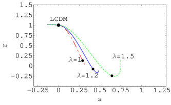
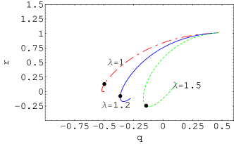
Figure 1: The left figure is $s-r$ diagram of attractor solution in quintessence model. The right figure is $q-r$ diagram of attractor solution in quintessence model. The curves evolve in the variable interval $N\in[-2,10]$. Selected curves for $\gamma_{m}=1$, $\lambda=1$, $1.2$ and $1.5$ respectively. Dots locate the current values of the statefinder parameters.

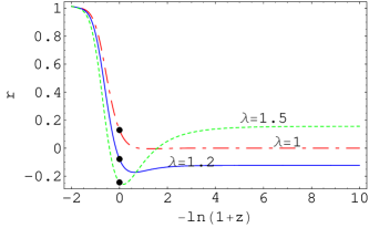
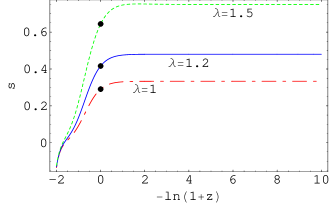
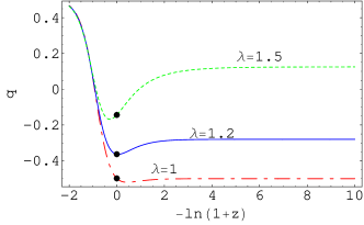
Figure 2: The figures are the statefinder parameters and deceleration parameter versus redshift diagram of the attractor solution in quintessence model. The left figure is $-\ln(1+z)$ — $r$ diagram, the middle figure is $-\ln(1+z)$ — $s$ diagram and the right figure is $-\ln(1+z)$ — $q$ diagram. The curves evolve in the variable interval $N\in[-2,10]$. Selected curves for $\gamma_{m}=1$, $\lambda=1$, $1.2$ and $1.5$ respectively. Dots locate the current values of the statefinder parameters.

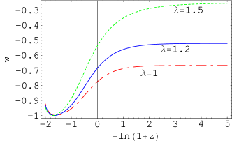
Figure 3: The figures are the equation of state of the quintessence model $w$ versus redshift. The curves evolve in the variable interval $N\in[-2,5]$. Selected curves for $\gamma_{m}=1$, $\lambda=1$, $1.2$ and $1.5$ respectively.

IV Statefinder Parameter for 5D Attractor Solution of Phantom Model

The phantom model is the scenario of equations (8)-(10) with $\varepsilon=-1$, which has been discussed in previous work phattractor2 . As in Ref. phattractor2 , we define the dimensionless variables:

$$x=\frac{\kappa\dot{\phi}}{\sqrt{6}BH},\qquad\qquad y=\frac{\kappa\sqrt{V}}{\sqrt{3}H}.$$ (17)

For a spatially flat universe $(k=0)$, we find that the evolution equation for $x$ and $y$ in the phantom model are:

$$x^{{}^{\prime}} = \frac{3}{2}x[-2x^{2}+\gamma_{m}(1+x^{2}-y^{2})]-3x-\lambda\sqrt{\frac{3}{2}}y^{2},$$

$$y^{{}^{\prime}} = \frac{3}{2}y[-2x^{2}+\gamma_{m}(1+x^{2}-y^{2})]-\lambda\sqrt{\frac{3}{2}}xy.$$ (18)

where a prime denotes a derivative with respect to the logarithm of the scale factor, $N=\ln A$. And we can get the densities of two components:

$$\Omega_{m}=\frac{\kappa^{2}\rho_{m}}{3H^{2}}=1+x^{2}-y^{2},\qquad\qquad\Omega_{\phi}=\frac{\kappa^{2}\rho_{\phi}}{3H^{2}}=-x^{2}+y^{2}.$$ (19)

and the equation of state parameter for phantom is:

$$w_{\phi}=\frac{x^{2}+y^{2}}{x^{2}-y^{2}}.$$ (20)

The statefinder parameters and deceleration parameter for this phantom model are:

$$r = (\frac{9}{2}\gamma_{m}^{2}-\frac{9}{2}\gamma_{m}+1)(1+x^{2}-y^{2})-3\sqrt{6}{\lambda}xy^{2}-10x^{2}+y^{2},$$

$$s = \frac{(\frac{9}{2}\gamma_{m}^{2}-\frac{9}{2}\gamma_{m}+1)(1+x^{2}-y^{2})-3\sqrt{6}{\lambda}xy^{2}-10x^{2}+y^{2}-1}{3[(\frac{3}{2}\gamma_{m}-1)(1+x^{2}-y^{2})-2x^{2}-y^{2}-\frac{1}{2}]},$$

$$q = (\frac{3}{2}\gamma_{m}-1)(1+x^{2}-y^{2})-2x^{2}-y^{2},$$ (21)

There is only one meaningful late-time attractor solution for (18), which is the scalar field dominated solution:

$$x=-\lambda/\sqrt{6},\qquad\qquad y=\sqrt{1+\lambda^{2}/6}.$$ (22)

and the eigenvalue of this solution is $(-3-\lambda^{2}/2,-3\gamma_{m}-\lambda^{2})$.

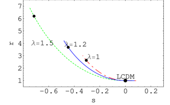
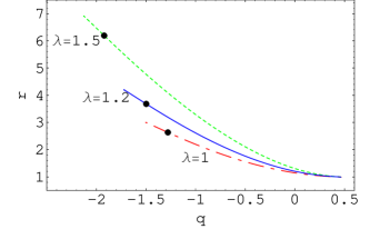
Figure 4: The left figure is $s-r$ diagram of attractor solution in phantom model. The right figure is $q-r$ diagram of attractor solution in phantom model. The curves evolve in the variable interval $N\in[-2,10]$. Selected curves for $\gamma_{m}=1$, $\lambda=1$, $1.2$ and $1.5$ respectively. Dots locate the current values of the statefinder parameters.

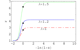
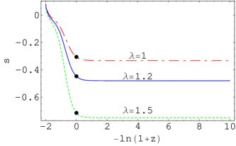
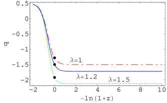
Figure 5: The figures are the statefinder parameters and deceleration parameter versus redshift diagram of the attractor solution in phantom model. The left figure is $-\ln(1+z)$ — $r$ diagram, the middle figure is $-\ln(1+z)$ — $s$ diagram and the right figure is $-\ln(1+z)$ — $q$ diagram. The curves evolve in the variable interval $N\in[-2,10]$. Selected curves for $\gamma_{m}=1$, $\lambda=1$, $1.2$ and $1.5$ respectively. Dots locate the current values of the statefinder parameters.

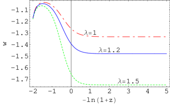
Figure 6: The figures are the equation of state of the phantom model $w$ versus redshift. The curves evolve in the variable interval $N\in[-2,5]$. Selected curves for $\gamma_{m}=1$, $\lambda=1$, $1.2$ and $1.5$ respectively.

In Fig. 4 we show the time evolution of the statefinder pairs $\{r,s\}$ and $\{r,q\}$ for the attractor solution of the phantom field. The plot is also for variable interval $N\in[-2,10]$, and the corresponding parameters are the same in the Fig. 1. We also can see that the curves far from the LCDM in the future, but the statefinder pair $\{r,s\}$ lies in the region $s<0$, $r>1$ which is different from that in Fig. 1. We see that the statefinder trajectories $r-s$ is almost linear in the past and future, which means that the deceleration parameter changes from one constant to another nearly with the increasing of the time, which can also be seen from the Fig. 6. In Fig. 5, the curves of $-ln(1+z)$ — $r$ and $-ln(1+z)$ — $s$ show clearly that the parameter $r$ will apart from $1$ and $s$ will far from $0$ with the increase of the parameter $\lambda$. From $-ln(1+z)$ — $q$ diagram we can found that the deceleration parameter $q$ of phantom are all satisfy $q<-1$ with different parameter $\lambda$ at present. In Fig. 6 we see that the equation of state of phantom below $-1$, which is different from the Fig. 3, and which could cause a big rip big rip ; big rip1 in the universe in the future.
We have applied a statefinder analysis to the 5D attractor solutions of quintessence and phantom field, and investigate the effect of the parameter $\lambda$ in the potential $V(\phi)$. Though these two attractor solutions are both scalar field dominated solution, the difference of these two solutions can be found in the statefinder parameters plane Fig.1-Fig.6: (i) The region of the statefinder pair $\{r,s\}$ is different between Fig. 1 and Fig. 4. For quintessence scenario Fig. 1, $s>0$ and $r<1$ while for phantom scenario Fig. 4, $s<0$ and $r>1$. (ii) The influence of the parameter $\lambda$ in potential $V(\phi)$ is different in the evolution of the universe, which can be seen in the statefinder trajectories. In quintessence scenario Fig. 2, the increasing of the $\lambda$ will decrease the statefinder parameter $r$ and the deceleration parameter $q$, while it will increase the statefinder parameter $s$. In phantom scenario Fig. 4, the statefinder parameter $r$ will be increased, while the $s$ and $q$ will be decreased with the increasing of the $\lambda$ in the potential. So, through the statefinder parameter, we can see the difference between quintessence field and phantom field clearly. The attractor solution of quintessence field will cause the universe to accelerate forever, but, the attractor solution of phantom field will cause the universe to end with a big rip. So, We think that we should pay attention to find a suitable interaction between phantom and dark matter or other components in 5D model to avoid the big rip in our future work.

V Discussion

In summary, we have studied the statefinder parameter $r$ and $s$ in the five-dimensional big bounce model in a plane-autonomous system, and apply it to contrast the attractor solution of the quintessence field and the phantom field respectively. It is found that the evolving trajectories of these two attractor solutions in the $\{r,s\}$ and $\{r,q\}$ plane is quite different, and which is also different from the statefinder diagnostic of other dark models. Through the figures of the statefinder parameters and deceleration parameter we can see that the universe will accelerate forever in the quintessence scenario, while the universe will end with a big rip in the phantom scenario. We hope that the future high precision observation will be able to determine these statefinder parameters and consequently shed light on the nature of dark energy.

VI Acknowledgments

This work was supported by NSF (10573003), NBRP (2003CB716300) of P. R. China and DUT 893321.

VII References

References

- (1) D. N. Spergel, et. al, Astrophys. J. Supp. 148 175 (2003), astro-ph/0302209.
- (2) A. G. Riesset, et. al, Astron. J. 116 1009 (1998), astro-ph/9805201.
- (3) A. C. Pope, et. al, Astrophys.J. 607 655 (2004), astro-ph/0401249.
- (4) V. Sahni, A. Starobinsky, Int. J. Mod. Phys. D9, 373-444 (2000), astro-ph/9904398.
- (5) S. Weinberg, Rev. Mod. Phys. 61, 1 (1989).
- (6) S. M. Carroll, Living Rev. Rel. 4, 1 (2001), astro-ph/0004075.
- (7) P. J. E. Peebles and B. Ratra, Rev. Mod. Phys. 75, 559 (2003), astro-ph/0207347.
- (8) T. Padmanabhan, Phys. Rept. 380, 235 (2003), hep-th/0212290.
- (9) B. Ratra and P. J. Peebles, Phys. Rev. D37 3406 (1988).
- (10) R. R. Caldwell, R. Dave and P. J. Steinhardt, Phys. Rev. Lett. 80, 1582 (1998).
- (11) M. S. Turner , Int. J. Mod. Phys. A17S1, 180 (2002), astro-ph/0202008.
- (12) V. Sahni , Class. Quant. Grav. 19, 3435 (2002), astro-ph/0202076.
- (13) I. Zlatev, L. Wang, and P. J. Steinhardt , Phys. Rev. Lett. 82, 896 (1999), astro-ph/9807002.
- (14) P. J. Steinhardt, L. Wang , I. Zlatev, Phys. Rev. D59, 123504 (1999), astro-ph/9812313.
- (15) X. Zhang, Mod. Phys. Lett. A20, 2575 (2005), astro-ph/0503072.
- (16) R. R. Caldwell, M. Kamionkowski, N. N. Weinberg, Phys. Rev. Lett. 91, 071301 (2003), astro-ph/0302506.
- (17) P. Singh, M. Sami, N. Dadhich, Phys. Rev. D68, 023522 (2003), hep-th/0305110.
- (18) J. G. Hao, X. Z. Li, Phys. Rev. D67, 107303 (2003), gr-qc/0302100.
- (19) Z. K. Guo, Y. S. Piao and Y. Z. Zhang, Phys. Lett. B594, 247-251 (2004), astro-ph/0404225.
- (20) L. X. Xu, H. Y. Liu, Int. J. Mod. Phys. D14, 1947-1957 (2005), astro-ph/0507250.
- (21) S. C. C. Ng, N. J. Nunes and F. Rosati, Phys. Rev. D64, 083510 (2001).
- (22) E. J. Copeland, A. R. Liddle and D. Wands, Phys. Rev. D57, 4686 (1998).
- (23) B. R. Chang, H. Y. Liu and L. X. Xu, Mod. Phys. Lett. A20, 923 (2005), astro-ph/0405084.
- (24) J. G. Hao and X. Z. Li, Phys. Rev. D67, 107303 (2003).
- (25) X. Z. Li and J. G. Hao, Astrophys. J. 592, 767-781 (2003), hep-th/0303093.
- (26) J. G. Hao, X. Z. Li, Phys. Rev. D70, 043529 (2004), astro-ph/0309746.
- (27) H. Y. Liu, H. Y. Liu, B. R. Chang and L. X. Xu, Mod. Phys. Lett. A20, 1973-1982 (2005), gr-qc/0504021.
- (28) V. Sahni, T. D. Saini, A. A. Starobinsky and U. Alam, JETP Lett. 77, 201 (2003), astro-ph/0201498.
- (29) W. Zimdahl and D. Pavon, Gen. Rel. Grav. 36, (2004) 1483.
- (30) U. Alam, V. Sahni, T. D. Saini and A. A. Starobinsky, Mon. Not. Roy. ast. Soc. 344, (2003) 1057, astro-ph/0303009.
- (31) V. Gorini, A. Kamenshchik and U. Moschella, Phys. Rev. D67, (2003) 063509, astro-ph/0209395.
- (32) X. Zhang, Phys. Lett. B611, 1 (2005), astro-ph/0503075.
- (33) X. Zhang, Int. J. Mod. Phys. D14, 1597 (2005), astro-ph/0504586.
- (34) P. X. Wu and H. W. Yu, Int. J. Mod. Phys. D14, 1873-1882 (2005), gr-qc/0509036.
- (35) X. Zhang, F. Q. Wu, J. F. Zhang, JCAP 0601, 003 (2006), astro-ph/0411221.
- (36) B. R. Chang, H. Y. Liu, L. X. Xu, C. W. Zhang and Y. L. Ping, JCAP 0701, 016 (2007), astro-ph/0612616.
- (37) H. Y. Liu and P. S. Wesson, Astrophys. J. 562, 1 (2001), gr-qc/0107093.
- (38) T. Liko and P. S. Wesson, gr-qc/0310067.
- (39) H. Y. Liu, Phys. Lett. B560, 149 (2003), hep-th/0206198.
- (40) B. L. Wang, H. Y. Liu and L. X. Xu, Mod. Phys. Lett. A19, 449 (2004), gr-qc/0304093.
- (41) X. L. Xin, H. Y. Liu and B. L. Wang, Chin. Phys. Lett. 20, 995 (2003), gr-qc/0304049.
- (42) L. X. Xu and H. Y. Liu, Int. J. Mod. Phys. D14, 883-892 (2005), astro-ph/0412241.
- (43) L. X. Xu, H. Y. Liu and B. R. Chang, Mod. Phys. Lett. A20, 3105-3114 (2005), astro-ph/0507397.
- (44) L. X. Xu, H. Y. Liu and C. W. Zhang, Int. J. Mod. Phys. D15, 215-224 (2006), astro-ph/0510673.
- (45) L. X. Xu, H. Y. Liu and Y. L. Ping, Int. J. Theor. Phys. 45, 843-850 (2006), astro-ph/0601471.
- (46) C. W. Zhang, H. Y. Liu, L. X. Xu and P. S. Wesson, Mod. Phys. Lett. A21, 571-580 (2006), astro-ph/0602414.
- (47) Y. L. Ping, H. Y. Liu, L. X. Xu, Int. J. Mod. Phys. A22, 985 (2007), gr-qc/0610094.
- (48) M. L. Liu, H. Y. Liu, L. X. Xu, Paul S. Wesson, Mod. Phys. Lett. A21, 2937 (2006), gr-qc/0611137.
- (49) J. M. Overduin and P. S. Wesson, Phys. Rep. 283 , 303 (1997), gr-qc/9805018.
- (50) P. S. Wesson, Space-Time-Matter (World Scientific, 1999).
- (51) J. E. Campbell, A Course of Differential Geometry (Clarendon, 1926).
- (52) H. Y. Liu and B. Mashhoon, Ann. Phys. 4, 565 (1995).
- (53) J. G. Hao and X. Z. Li, Phys. Rev. D68, (2003) 083514, hep-th0306033.
- (54) Z. K. Guo, Y. S. Piao, Y. Z. Zhang, Phys. Lett. B594, (2004) 247-251, astro-ph/0404225.