Quantum Darwinism in quantum Brownian motion: the vacuum as a witness

Abstract

We study quantum Darwinism – the redundant recording of information about a decohering system by its environment – in zero-temperature quantum Brownian motion. An initially nonlocal quantum state leaves a record whose redundancy increases rapidly with its spatial extent. Significant delocalization (e.g., a Schrödinger’s Cat state) causes high redundancy: Many observers can measure the system’s position without perturbing it. This explains the objective (i.e. classical) existence of einselected, decoherence-resistant pointer states of macroscopic objects.

A quantum system ($\mathcal{S}$) decoheres when monitored by its environment ($\mathcal{E}$) Paz and Zurek (2001) Zurek (2003). That environment can act as a “witness”, recording information about $\mathcal{S}$. When many copies exist, the information is redundant, and effectively objective: many observers can obtain it, but no one can change or erase it. Objective existence is a defining feature of classical reality. When information about one observable is redundant, information about complementary observables becomes inaccessible and it effectively ceases to exist Zurek (2003); Ollivier et al. (2004); Blume-Kohout and Zurek (2006). This selective proliferation of “fit” information, at the expense of incompatible (complementary) information, is quantum Darwinism.

In this paper, we demonstrate quantum Darwinism in zero temperature quantum Brownian motion (QBM). A harmonic oscillator system ($\mathcal{S}$) evolves in contact with a bath ($\mathcal{E}$) of harmonic oscillators. We focus on the macroscopic regime, where the system is massive and underdamped. In this limit, we show how redundancy increases with the spatial extent of system’s wavefunction, so that many fragments of $\mathcal{E}$ “know” the location of $\mathcal{S}$.

To study how information about $\mathcal{S}$ appears redundantly in $\mathcal{E}$ during decoherence we must analyze the state of $\mathcal{E}$, not trace it out. In this “environment as a witness” paradigm, $\mathcal{E}$ is not a sink for information, but a resource from which it might be extracted. Quantum Darwinism was introduced recently (see Zurek (2003) and references therein), and investigated in Ollivier et al. (2004). Here, we pursue the formulation of Blume-Kohout and Zurek (2006).

The core question is “How much information about $\mathcal{S}$ can an observer extract from $\mathcal{E}$?” $\mathcal{E}$ consists of subenvironments $\mathcal{E}_{i}$ ($\mathcal{E}$ = $\mathcal{E}_{1}\otimes\mathcal{E}_{2}\otimes\mathcal{E}_{3}\ldots$). Each observer has exclusive access to a fragment $\mathcal{F}$ comprising $m$ subenvironments (see Fig. 1). We factor the QBM bath into its component oscillators or bands. This fixed decomposition, which breaks unitary invariance and is justified by $\mathcal{E}$’s interaction with apparatus, is essential Blume-Kohout and Zurek (2006).

We measure “information” by the quantum mutual information between $\mathcal{S}$ and $\mathcal{F}$,

$$\mathcal{I}_{\mathcal{S}:\mathcal{F}}=H_{\mathcal{S}}+H_{\mathcal{F}}-H_{\mathcal{S}\mathcal{F}},$$ (1)

where $H$ is the von Neumann entropy of a reduced density matrix. $\mathcal{I}_{\mathcal{S}:\mathcal{F}}$ is an upper bound for the entropy (in $\mathcal{S}$) eliminated by measuring $\mathcal{F}$. The bound is tight for classical correlations, but quantum correlations raise $\mathcal{I}_{\mathcal{S}:\mathcal{F}}$ above classically-allowed values. This quantum discord Ollivier and Zurek (2002) represents the ability to choose between several non-commuting observables (e.g., of $\mathcal{S}$). In presence of decoherence (inflicted on the $\mathcal{S}\mathcal{F}$ pair by the rest of $\mathcal{E}$) discord is expected to be small Zurek (2003); Ollivier and Zurek (2002).

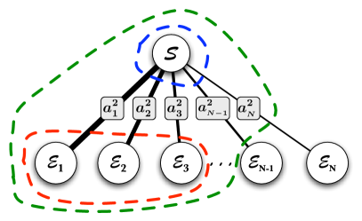
Figure 1: Information about the system can be extracted from fragments – collections of environment subsystems. In QBM, in the weak-dissipation limit, evolved states of $\mathcal{S}$ and $\mathcal{E}$ reflect the structure of the interaction Hamiltonian. Each band $\mathcal{E}_{\omega}$ of $\mathcal{E}$ develops independent correlations with $\mathcal{S}$ (black lines), quantified by extra squared symplectic area ($a^{2}_{\omega}$) induced in $\mathcal{S}$ and $\mathcal{E}_{\omega}$. A fragment $\mathcal{F}$ (red) comprises several (not necessarily contiguous) bands. $\mathcal{S}$ itself (blue) and the joint $\mathcal{S}\otimes\mathcal{F}$ (green) are also fragments. Symplectic area is approximately additive, so $a^{2}_{\mathcal{F}}$ is a sum over edges connected to $\mathcal{F}$. We use $a^{2}$ to compute entropy, and thence mutual information $\mathcal{I}_{\mathcal{S}:\mathcal{F}}$.

Figure 2: Delocalized states of a decohering oscillator ($\mathcal{S}$) are redundantly recorded by the environment ($\mathcal{E}$). Plot (a) shows redundancy ($R_{\delta}$) vs. imprecision ($\delta$), when $\left|\scriptstyle\psi(0)\right\rangle$ is squeezed in $x$ by $s_{x}=6.3\times 10^{3}$. Plots (b-d) show $R_{10\%}$ – redundancy of 90% of the available information – vs. initial squeezing ($s_{x}$ or $s_{p}$). Dots denote numerics; lines – our theory. Details: $\mathcal{S}$ has mass $m_{\scriptscriptstyle\mathcal{S}}=1000$, $\omega_{\scriptscriptstyle\mathcal{S}}=4$. $\mathcal{E}$ comprises oscillators with $\omega\in[0\ldots 16]$ and mass $m=1$. The frictional (coupling) frequency is $\gamma=\frac{1}{40}$. Discussion: Redundancy develops with decoherence: $p$-squeezed states [plot (c)] decohere almost instantly, while $x$-squeezed states [plot (b)] decohere as a $\frac{\pi}{2}$ rotation transforms them into $p$-squeezed states. Redundancy persists thereafter [plot (d)]; dissipation intrudes by $t\sim O(\gamma^{-1})$, causing $R_{10\%}$ to rise above our simple theory. Redundancy increases exponentially – as $R_{\delta}\approx s^{2\delta}$ – with imprecision [plot (a)]. So, while $R_{\delta}\sim 10$ may seem modest, $\delta=0.1$ implies very precise knowledge (resolution around 3 ground-state widths) of $\mathcal{S}$. This is half an order of magnitude better than a recent record LaHaye et al. (2004) for measuring a micromechanical oscillator. At $\delta\sim 0.5$ – resolving $\sim\sqrt{s}$ different locations within the wavepacket – $R_{50\%}\gtrsim 10^{3}$ (our maximum numerical resolution).

We use two tools to analyze information storage. Partial information is the average information in a random fragment containing a fraction $f$ of $\mathcal{E}$,

$$\overline{\mathcal{I}}(f)=\mathrm{avg}_{\mathrm{all\ }\mathcal{F}\mathrm{\ of\ size\ }f}\left(\mathcal{I}_{\mathcal{S}:\mathcal{F}}\right),$$ (2)

Partial information plots (PIPs) assume a characteristic shape in the presence of redundancy: $\overline{\mathcal{I}}(f)$ increases sharply around $f=0$ and $f=1$, but has a long, flat “classical plateau” in between. Thus, almost all (all but $\delta$) of this classical information can be extracted from a small fraction $f_{\delta}$ of $\mathcal{E}$. Redundancy ($R_{\delta}$) is just the number of disjoint fragments $\mathcal{F}$ that provide all but $\delta$ of the available information about $\mathcal{S}$ – i.e., satisfying $\mathcal{I}_{\mathcal{S}:\mathcal{F}}\geq(1-\delta)H_{\mathcal{S}}$, or;

$$R_{\delta}=\frac{1}{f_{\delta}}$$ (3)

Further discussion of $R_{\delta}$ and PIPs (see Figs. 2, 3), is found in Blume-Kohout and Zurek (2006).

The QBM Feynman and Vernon (1963); Caldeira and Leggett (1983); Unruh and Zurek (1989); Hu et al. (1992) Hamiltonian

$$\mathbf{{H}}=\mathbf{{H}}_{\mathrm{sys}}+\frac{1}{2}\sum_{\omega}{\left(\frac{q_{\omega}^{2}}{m_{\omega}}+m_{\omega}\omega^{2}y_{\omega}^{2}\right)}+x_{\mathcal{S}}\sum_{\omega}{C_{\omega}y_{\omega}}.$$ (4)

describes a central oscillator whose position $x_{\mathcal{S}}$ is linearly coupled to a bath of oscillators. The central system obeys $\mathbf{{H}}_{\mathrm{sys}}=(\frac{p_{\mathcal{S}}^{2}}{m_{\scriptscriptstyle\mathcal{S}}}+m_{\scriptscriptstyle\mathcal{S}}\Omega_{0}^{2}x_{\mathcal{S}}^{2})/2$; the environmental coordinates $y_{\omega}$ and $q_{\omega}$ describe a single band (oscillator) $\mathcal{E}_{\omega}$. As usual, the bath is defined by its spectral density, $I(\omega)=\sum_{n}{\delta\left(\omega-\omega_{n}\right)\frac{C_{n}^{2}}{2m_{n}\omega_{n}}},$ which quantifies the coupling between $\mathcal{S}$ and each band of $\mathcal{E}$. We consider an ohmic bath with a cutoff $\Lambda$ (see note ): $I(\omega)=\frac{2m_{\scriptscriptstyle\mathcal{S}}\gamma_{0}}{\pi}\omega$ for $\omega\in[0\ldots\Lambda]$. Each coupling is a differential element, $\mathrm{d}C_{\omega}^{2}=\frac{4m_{\scriptscriptstyle\mathcal{S}}m_{\omega}\gamma_{0}}{\pi}\omega^{2}\mathrm{d}\omega$ for $\omega\in[0\ldots\Lambda]$. For numerics, we divide $[0\ldots\Lambda]$ into discrete bands of width $\Delta\omega$, which approximates the exact model well up to a time $\tau_{rec}\sim\frac{2\pi}{\Delta\omega}$.

We initialize $\mathcal{S}$ in a squeezed coherent state, and $\mathcal{E}$ in its ground state. QBM’s linear dynamics preserve the Gaussianity of the initial state, which can be described by its mean and variance:

$$\vec{z}=\left(\begin{array}[]{c}\left\langle x\right\rangle\\ \left\langle p\right\rangle\end{array}\right)\mbox{\ ;\ }\Delta=\left(\begin{array}[]{cc}\Delta x^{2}&\Delta xp\\ \Delta xp&\Delta p^{2}\end{array}\right).$$ (5)

Its entropy, $H(\rho)=-\mathrm{Tr}\rho\ln\rho$, is a function of its squared symplectic area,

$$a^{2}=\left(\frac{\hbar}{2}\right)^{-2}\det(\Delta)$$ (6)

$$H(a)=\frac{1}{2}\left(\begin{array}[]{l}\ (a+1)\ln(a+1)\\ -(a-1)\ln(a-1)\end{array}\right)-\ln 2\approx\ln\left(\frac{e}{2}a\right),$$ (9)

where $e$ is Euler’s constant, and the approximation is excellent for $a>2$. For multi-mode states, numerics yield $H(\rho)$ exactly as a sum over $\Delta$’s symplectic eigenvalues Serafini et al. (2004), but our theoretical treatment approximates a collection of oscillators as a single mode with a single $a^{2}$.

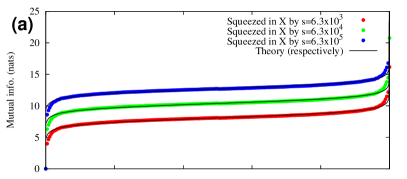
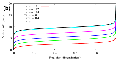
Figure 3: Partial information plots (PIPs) show how information is stored in $\mathcal{E}$. They illustrate how $\mathcal{I}_{\mathcal{S}:\mathcal{F}}$ – the amount of information in a randomly chosen fragment $\mathcal{F}\subset\mathcal{E}$ – depends on $\mathcal{F}$’s size. Here, we initialized $\mathcal{S}$ in an $x$-squeezed state, which decoheres as it evolves into a superposition of $x$ states. Plot (a) shows PIPs for three fully-decohered ($t=4$) states with different squeezing. Small fragments of $\mathcal{E}$ provides most of the available information about $\mathcal{S}$; squeezing changes the amount of redundant information without changing the PIP’s shape. The numerics agree with a simple theory. Plot (b) tracks one state as decoherence progresses. Again, PIPs’ shape is invariant; time only changes the amount of redundant information.

Exact solutions to QBM, even for the reduced dynamics of $\mathcal{S}$ alone, are nontrivial. Quantum Darwinism requires a more extensive solution describing the dynamics of $\mathcal{E}$. We obtain it numerically, describing the initial Gaussian product state with a covariance matrix (Eq. 5), evolving it by canonical methods (see Anglin and Habib (1996); Blume-Kohout and Zurek (2003)), and computing mutual information from symplectic area. To compute redundancy ($R_{\delta}$), we apply a Monte Carlo technique to find the amount of randomly selected bandwidth required to obtain $\mathcal{I}_{\mathcal{S}:\mathcal{F}}=(1-\delta)H_{\mathcal{S}}$. We choose units where: $\frac{\hbar}{2}=1$; the masses of the $\mathcal{E}_{\omega}$ are 1; the renormalized frequency of $\mathcal{S}$ is 4; and the bath frequencies lie in $[0,\Lambda=16]$. The frictional coefficient $\gamma_{0}$ varies with $m_{\scriptscriptstyle\mathcal{S}}$ so that $m_{\scriptscriptstyle\mathcal{S}}\gamma_{0}=25$; most often, $m_{\scriptscriptstyle\mathcal{S}}=10^{3}$ and $\gamma_{0}=\frac{1}{40}$.

Our main result is that substantial redundancy appears in the QBM model (Fig. 2). Redundancy depends on the initial squeezing $s$, so that $R_{\delta}\sim s^{2\delta}$. It appears along with decoherence – rapidly for $\hat{p}$-squeezed states (Fig. 2b), more slowly for $\hat{x}$-squeezed states (Fig. 2a) – then remains relatively constant. However, dissipation (not analyzed here) causes redundancy to further increase on a timescale $t\sim O(\gamma_{0}^{-1})$ (see Fig. 2d).

PIPs (Fig. 3) show how information about $\mathcal{S}$ is stored in $\mathcal{E}$. $\overline{\mathcal{I}}(f)$ rises rapidly as the fragment’s size ($f$) increases from zero, then flattens for larger fragments. Most – all but $\sim 1$ nat – of $H_{\mathcal{S}}$ is redundant. When $\mathcal{S}$ is macroscopic, this non-redundant information is dwarfed by the total amount of information lost to $\mathcal{E}$.

Let us now derive a model for this behavior. Suppose $\mathcal{S}$ is macroscopic, so $m_{\scriptscriptstyle\mathcal{S}}\rightarrow\infty$. The bath’s spectral density is independent of $m_{\scriptscriptstyle\mathcal{S}}$, so $m_{\scriptscriptstyle\mathcal{S}}\gamma_{0}$ remains constant, and $\gamma_{0}$ is small. The mutual information between $\mathcal{S}$ and a fragment $\mathcal{F}$ depends on the entropies of $\rho_{\mathcal{S}}$, $\rho_{\mathcal{F}}$, and $\rho_{\mathcal{S}\mathcal{F}}$, so we compute their squared symplectic areas.

As $m_{\scriptscriptstyle\mathcal{S}}\rightarrow\infty$, the kinetic term in $\mathbf{{H}}_{\mathrm{sys}}$ (Eq. 4) becomes insignificant. $\mathbf{{H}}_{\mathrm{sys}}$ thus commutes with the interaction term, and can be ignored. The remainder of $\mathbf{{H}}$ has the form $1\!\mathrm{l}_{\mathcal{S}}\otimes\sum_{\omega}{\mathbf{{H}}_{\omega}}+\hat{}x_{\mathcal{S}}\otimes\sum_{\omega}{\mathbf{R}_{\omega}}$. When $\left|\scriptstyle\psi_{\mathcal{S}}\right\rangle=\left|\scriptstyle x\right\rangle$, each $\mathcal{E}_{\omega}$ feels a well-defined $\mathbf{{H}}_{\omega}(x)$, and evolves as $\left|\scriptstyle\psi_{\omega}(0)\right\rangle\rightarrow\left|\scriptstyle\psi_{\omega}(t;x)\right\rangle$, conditional upon the value of $x$. When $\left|\scriptstyle\psi_{\mathcal{S}}(0)\right\rangle$ is a superposition of $\left|\scriptstyle x\right\rangle$ states, the product state evolves into a Gaussian singly-branching state Blume-Kohout and Zurek (2006);

$$\left(\int{\!\psi_{\mathcal{S}}(x)\left|\scriptstyle x\right\rangle\mathrm{d}x}\right)\otimes\left|\scriptstyle\psi_{1}(0)\right\rangle\left|\scriptstyle\psi_{2}(0)\right\rangle\ldots\left|\scriptstyle\psi_{N_{\mathrm{env}}}(0)\right\rangle$$ (10)

$$\Downarrow$$

$$\int{\psi_{\mathcal{S}}(x)\left|\scriptstyle x\right\rangle\otimes\left|\scriptstyle\psi_{1}(t;x)\right\rangle\left|\scriptstyle\psi_{2}(t;x)\right\rangle\ldots\left|\scriptstyle\psi_{N_{\mathrm{env}}}(t;x)\right\rangle\mathrm{d}{x}},$$ (11)

The reduced state $\rho_{\mathcal{A}}$ for any subsystem $\mathcal{A}$ is spectrally equivalent to a partially-decohered state of $\mathcal{S}$:

$$\rho_{\mathcal{A}}(x,x^{\prime})=\rho_{\mathcal{S}}(x,x^{\prime},t=0)\Gamma_{\mathcal{A}}(x,x^{\prime}).$$ (12)

The decoherence factor $\Gamma_{\mathcal{A}}(x,x^{\prime})$ is a product (over all $\mathcal{E}_{\omega}$ not in $\mathcal{A}$ if $\mathcal{A}$ contains $\mathcal{S}$; otherwise, over all $\mathcal{E}_{\omega}$ in $\mathcal{A}$) of contributions $\Gamma_{\omega}(x,x^{\prime})\equiv\left\langle\scriptstyle\psi_{\omega}(t;x)|\psi_{\omega}(t;x^{\prime})\right\rangle$ from individual bands.

$\Gamma_{\omega}(x,x^{\prime})$ measures a band’s power to decohere $\left|\scriptstyle x\right\rangle$ from $\left|\scriptstyle x^{\prime}\right\rangle$. Let us define an additive decoherence factor $d\propto\log\Gamma$. The logarithm is always proportional to $(x-x^{\prime})^{2}$ (see Eq. 16), so we set

$$d_{\omega}(t)\equiv-\frac{\log\left(\Gamma_{\omega}(x,x^{\prime})\right)}{(x-x^{\prime})^{2}}.$$ (13)

For a continuous spectral density, $d_{\omega}$ is a differential $\mathrm{d}d_{\omega}=\frac{\mathrm{d}d}{\mathrm{d}\omega}\mathrm{d}\omega$, and the decoherence $d_{\mathcal{A}}$ experienced by a subsystem $\mathcal{A}$ is an integral over its bandwidth.

Suppressing off-diagonal elements of $\rho$ affects $\hat{x}$ not at all, but increases $\Delta p^{2}$ by $\delta p^{2}_{\mathcal{A}}=2\hbar d_{\mathcal{A}}$, so

$$a^{2}_{\mathcal{A}}\rightarrow 1+\delta a^{2}_{\mathcal{A}}=1+\left(\frac{\hbar}{2}\right)^{-2}\Delta x^{2}\delta p^{2}_{\mathcal{A}}=1+\frac{8\Delta x^{2}}{\hbar}d_{\mathcal{A}}.$$ (14)

This $\delta a^{2}$ is a key quantity. It measures the correlation-induced uncertainty in $\mathcal{A}$ and its complement, and therefore the amount of correlation. For example, the correlation between $\mathcal{S}$ and $\mathcal{E}$ is the uncertainty in $\mathcal{S}$, given by an integral over all bands of $\mathcal{E}$: $\delta a^{2}_{\mathcal{S}}=\frac{8\Delta x^{2}}{\hbar}\int_{0}^{\Lambda}{\frac{\mathrm{d}d}{\mathrm{d}\omega}\mathrm{d}\omega}.$ The uncertainty in a fragment $\mathcal{F}$ is the integrated $\mathrm{d}a^{2}$ from all its component bands; that in $\mathcal{S}\mathcal{F}$ is the integrated $\mathrm{d}a^{2}$ for its complement, $\overline{\mathcal{F}}$ (where $\mathcal{E}=\mathcal{F}\otimes\overline{\mathcal{F}}$; see Fig. 1).

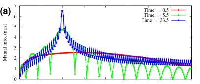
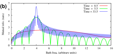
Figure 4: Different bands of $\mathcal{E}$ hold different amounts of information. Here, $\mathcal{S}$ is prepared with a squeezing of $s=6.3\times 10^{3}$, and the dissipation constant is $\gamma=\frac{1}{400}$. Plot (a) shows numerics, while (b) shows theory (see Eq. 17). Initially (red), all bands participate. Later (green), resonant bands around $\omega\sim\Omega=4$ become more important. After many oscillations (blue), resonant bands dominate. Theory agrees extremely well, though small discrepancies appear later.

When $\mathcal{S}$ is in state $\left|\scriptstyle x\right\rangle$, $\mathcal{E}_{\omega}$ experiences a Hamiltonian

$$\mathbf{{H}}_{\omega}(x)=\frac{q_{\omega}^{2}}{2m_{\omega}}+\frac{m_{\omega}\omega^{2}}{2}\left(y_{\omega}-\delta y_{\omega}\right)^{2}-\frac{m_{\omega}^{2}\omega^{2}}{2}\delta y_{\omega}^{2}.$$ (15)

Its initial (ground) state $\left|\scriptstyle\psi_{\omega}(0)\right\rangle$ evolves into a coherent state $\left|\scriptstyle\psi_{\omega}(t;x)\right\rangle$, along a circle of radius $\delta y_{\omega}=C_{\omega}/(m_{\omega}\omega^{2})$. Solving the equation of motion and inserting $\Delta y_{0}^{2}=\hbar/2m_{\omega}$ and $\Delta q_{0}^{2}=\hbar m_{\omega}/2$ yields

$$\left|\Gamma^{(\omega)}_{x,x^{\prime}}\right|=\exp\left[-\frac{C_{\omega}^{2}}{2m_{\omega}\hbar\omega^{3}}(x-x^{\prime})^{2}\left(1-\cos\omega t\right)\right].$$ (16)

The exponent is (as promised) proportional to $(x-x^{\prime})^{2}$, and $\mathrm{d}d_{\omega}=\frac{2m_{\scriptscriptstyle\mathcal{S}}\gamma_{0}}{\pi\hbar\omega}(1-\cos\omega t)\mathrm{d}\omega.$

Beyond $t\sim O(\omega_{\scriptscriptstyle\mathcal{S}}^{-1})$, $\mathbf{{H}}_{\mathrm{sys}}$ becomes relevant. $\mathcal{E}_{\omega}$ is driven, not just displaced, by $\mathcal{S}$. $\mathcal{S}$ is very massive, so it acts as a classical driving force on $\mathcal{E}_{\omega}$. To model this, we substitute $x=x_{0}\cos\omega_{\scriptscriptstyle\mathcal{S}}t$ into Eq. 15 and re-solve the ensuing equation of motion to get

$$\frac{\mathrm{d}d}{\mathrm{d}\omega}=\frac{m_{\scriptscriptstyle\mathcal{S}}\gamma_{0}}{\pi\hbar}\frac{\omega^{3}\mathrm{d}\omega}{(\omega_{\scriptscriptstyle\mathcal{S}}^{2}-\omega^{2})^{2}}\left[\begin{array}[]{l}\ \ \left(\sin\omega t-\frac{\omega_{\scriptscriptstyle\mathcal{S}}}{\omega}\sin\omega_{\scriptscriptstyle\mathcal{S}}t\right)^{2}\vspace{0.05in}\\ +(\cos\omega t-\cos\omega_{\scriptscriptstyle\mathcal{S}}t)^{2}\end{array}\right].$$ (17)

Integrating over $\omega$ yields a cumbersome formula for $\delta a^{2}_{\mathcal{S}}$, and thus for $H_{\mathcal{S}}(t)$.

We can now predict PIPs ($\overline{\mathcal{I}}(f)$). When $\mathcal{F}$ contains a randomly selected fraction $f$ of $\mathcal{E}$’s bandwidth, $\rho_{\mathcal{F}}$’s squared area is $a^{2}_{\mathcal{F}}=1+f\delta a^{2}_{\mathcal{S}}$, and that of $\rho_{\mathcal{S}\mathcal{F}}$ is $a^{2}_{\mathcal{S}\mathcal{F}}=1+(1-f)\delta a^{2}_{\mathcal{S}}$. Applying Eq. (9) (where $\delta a^{2}_{\mathcal{S}}\gg 1$) yields

$$\mathcal{I}_{\mathcal{S}:\mathcal{F}}\approx H_{\mathcal{S}}+\frac{1}{2}\ln\left(\frac{f}{1-f}\right).$$ (18)

This simple result fits numerics very well (pre-dissipation), and predicts the shape-invariance of PIPs.

We can also predict where information is stored in $\mathcal{E}$. If $\mathcal{E}_{\omega}$ is a band at frequency $\omega$, of width $\Delta\omega$, then $\mathcal{I}_{\mathcal{S}:\mathcal{E}_{\omega}}=H(\mathcal{S})+H(\mathcal{E}_{\omega})-H(\mathcal{S}\mathcal{E}_{\omega})\approx H(\mathcal{E}_{\omega})$. The band’s entropy is computed from its decoherence factor, $d_{\mathcal{E}_{\omega}}\approx\Delta\omega\frac{\mathrm{d}d}{\mathrm{d}\omega}$ (Eq. 17). The results agree with numerics (Fig. 4).

Redundancy counts the number of disjoint fragments with $\mathcal{I}_{\mathcal{S}:\mathcal{F}}\geq(1-\delta)H_{\mathcal{S}}$. Because $\mathcal{I}_{\mathcal{S}:\mathcal{F}}$ depends only on the fragment’s size ($f$), $\mathcal{I}_{\mathcal{S}:\mathcal{F}}\geq(1-\delta)H_{\mathcal{S}}$ iff $f\geq f_{\delta}=\frac{e^{-2\delta H_{\mathcal{S}}}}{1+e^{-2\delta H_{\mathcal{S}}}}$. $\mathcal{E}$ contains $N_{\delta}=1/f_{\delta}$ such fragments, so

$$R_{\delta}\approx e^{2\delta H_{\mathcal{S}}}\approx s^{2\delta}.$$ (19)

The second equality follows because an $s$-squeezed state decoheres to a mixed state with $H_{\mathcal{S}}\approx\ln s$. Eq. (19) is a succinct and easy-to-use summary of our results, and fits the data well (see Fig. 2). For instance, at $\delta=0.5$, we localize $\mathcal{S}$ with accuracy $\sim\sqrt{s}$, with redundancy $R_{0.5}\propto s$ (see Fig. 2c).

To generalize this result, observe that squeezing controls the initial spatial extent ($\Delta x_{\mathcal{S}}$), and that redundancy increases rapidly with $\Delta x_{\mathcal{S}}$. A fragment of $\mathcal{E}$ provides a fuzzy measurement of $\mathcal{S}$ (whose resolution increases with its size). A Schrödinger’s Cat state will yield high redundancy (but only $\sim 1$ bit of entropy), because small fragments are sufficient to resolve the two branches.

We have provided convincing evidence for quantum Darwinism in one of the most-studied models of decoherence. Our theory of the $\mathcal{S}-\mathcal{E}$ information flows, using singly-branching states, effectively models detailed numerics, and leads to a compelling picture: redundancy (e.g., Eq. 19) accounts for objectivity and classicality; the environment is a witness, holding many copies of the evidence. Though we did not discuss dissipation (which requires more sophisticated analysis), it actually increases $R_{\delta}$, by reducing non-redundant correlations. We postpone discussion of quantum Darwinism in the dissipative regime, and comparisons with the case of discrete pointer observables, to forthcoming papers.

We acknowledge stimulating discussions and useful comments on the manuscript by David Poulin.

References

Paz and Zurek (2001)
J. P. Paz and
W. H. Zurek,
Les Houches School
72, 535 (2001); E. Joos,
H. D. Zeh,
C. Kiefer,
D. Giulini,
J. Kupsch, and
I.-O. Stamatescu,
Decoherence and the appearance of a classical world in
quantum theory (New York: Springer,
2003), 2nd ed.; M. Schlosshauer,
Rev. Mod. Phys. 76,
1267 (2004).
Zurek (2003)
W. H. Zurek,
Rev. Mod. Phys. 75,
715 (2003); W. H. Zurek,
Annalen der Physik. 9,
855 (2000).
Ollivier et al. (2004)
H. Ollivier,
D. Poulin, and
W. H. Zurek,
Phys. Rev. Lett. 93,
220401 (2004); H. Ollivier,
D. Poulin, and
W. H. Zurek,
Phys. Rev. A 72,
042113 (2005).
Blume-Kohout and Zurek (2006)
R. Blume-Kohout
and W. H. Zurek,
Phys. Rev. A 73,
062310 (2006).
Ollivier and Zurek (2002)
H. Ollivier and
W. H. Zurek,
Phys. Rev. Lett. 88,
017901 (2002).
LaHaye et al. (2004)
M. D. LaHaye,
O. Buu,
B. Camarota, and
K. C. Schwab,
Science 304,
74 (2004).
Feynman and Vernon (1963)
R. P. Feynman and
F. L. Vernon,
Ann. Phys. 24,
118 (1963).
Caldeira and Leggett (1983)
A. O. Caldeira and
A. J. Leggett,
Physica A 121,
587 (1983).
Unruh and Zurek (1989)
W. G. Unruh and
W. H. Zurek,
Phys. Rev. D 40,
1071 (1989).
Hu et al. (1992)
B. L. Hu,
J. P. Paz, and
Y. H. Zhang,
Phys. Rev. D 45,
2843 (1992).
Serafini et al. (2004)
A. Serafini,
F. Illuminati,
and S. D. Siena,
J. Phys. B 37,
L21 (2004).
Anglin and Habib (1996)
J. R. Anglin and
S. Habib,
Mod. Phys. Lett. A 11,
2655 (1996).
Blume-Kohout and Zurek (2003)
R. Blume-Kohout
and W. H. Zurek,
Phys. Rev. A 68,
32104 (2003).