The Mean and Scatter of the velocity-dispersion–optical richness relation for maxBCG galaxy clusters
Abstract
The distribution of galaxies in position and velocity around the centers of galaxy clusters encodes important information about cluster mass and structure. Using the maxBCG galaxy cluster catalog identified from imaging data obtained in the Sloan Digital Sky Survey, we study the BCG–galaxy velocity correlation function. By modeling its non-Gaussianity, we measure the mean and scatter in velocity dispersion at fixed richness. The mean velocity dispersion increases from km s-1 for small groups to more than km s-1 for large clusters. We show the scatter to be at most %, declining to % in the richest bins. We test our methods in the C4 cluster catalog, a spectroscopic cluster catalog produced from the Sloan Digital Sky Survey DR2 spectroscopic sample, and in mock galaxy catalogs constructed from N-body simulations. Our methods are robust, measuring the scatter to well within one-sigma of the true value, and the mean to within 10%, in the mock catalogs. By convolving the scatter in velocity dispersion at fixed richness with the observed richness space density function, we measure the velocity dispersion function of the maxBCG galaxy clusters. Although velocity dispersion and richness do not form a true mass–observable relation, the relationship between velocity dispersion and mass is theoretically well characterized and has low scatter. Thus our results provide a key link between theory and observations up to the velocity bias between dark matter and galaxies.
Subject headings:
galaxies: clusters: general — cosmology — methods: data analysis1. Introduction
Galaxy clusters play an important role in observations of the large-scale structure of the Universe. As dramatically non-linear features in the matter distribution, they stand out as individually identifiable objects, whose abundant galaxies and hot X-ray emitting gas provide a rich variety of observable properties. Clusters can be identified by their galaxy content (Bahcall et al. 2003; Gladders & Yee 2005; Miller et al. 2005; Gerke et al. 2005; Berlind et al. 2006; Koester et al. 2007a, b), their thermal X-ray emission (Rosati et al. 1998; Böhringer et al. 2000; Popesso et al. 2004), the Sunyaev-Zeldovich decrement they produce in the microwave background signal (Grego et al. 2000; Lancaster et al. 2005), or the weak lensing signature they produce in the shapes of distant background galaxies (Wittman et al. 2006). Each of these identification methods also produces proxies for mass: e.g, the number of galaxies, total stellar luminosity, galaxy velocity dispersion, X-ray luminosity and temperature, or SZ and weak lensing profiles.
Simulations of the formation and evolution of large-scale structure through gravitational collapse provide us with rich predictions for the expected matter distribution within a given cosmology (Evrard et al. 2002; Springel et al. 2005). These predictions include not only first-order features, like the halo mass function n(M,z), but higher-order correlations as well, like the precise way in which galaxy clusters are themselves clustered as a function of mass. Comparisons of these theoretical predictions to the observed Universe provide an excellent opportunity to test our understanding of cosmology and the formation of large-scale structure. The weak point in this chain is that simulations most reliably predict the dark matter distribution, while observations are most directly sensitive to luminous galaxies and gas. Connections between observable properties and theoretical predictions for dark matter have often been made through simplifying assumptions that are hard to justify a priori.
Progress toward solving this problem has been made by the construction of various mass–observable scaling relations, which are based on combinations of theoretical predictions and observational measurements (Levine et al. 2002; Dahle 2006; Stanek et al. 2006). However, knowledge of the mean mass at a fixed value of the observable is not sufficient to extract precise cosmological constraints given the exponential shape of the halo mass function (Lima & Hu 2004, 2005). To perform precision cosmology, we must understand the scatter in the mass–observable relations as well.
Recently, Stanek et al. (2006) measured the scatter in the temperature-luminosity relation for X-ray selected galaxy clusters and used it to infer the scatter in the mass–luminosity relationship. Unfortunately, there are relatively few measurements of the scatter in any mass–observable relationship in the optical. (An exception is an early observation of scatter in the velocity-dispersion–richness relationship for a small sample of massive clusters by Mazure et al. 1996.) For optically selected clusters, the scatter is usually included as a parameter in the analysis (e.g. Gladders et al. 2007; Rozo et al. 2007a, b).
The primary goal of this work is to develop a method to estimate both the mean and scatter in the cluster velocity-dispersion–richness relation. This comparison between two observable quantities can be made without reference to structure formation theory. The method developed is applied to the SDSS maxBCG cluster catalog- a photometrically selected catalog with extensive spectroscopic follow-up. These methods are tested extensively with both the C4 catalog (Miller et al. 2005), a smaller spectroscopically-selected sample of clusters, and new mock catalogs generated by combining N-body simulations with a prescription for galaxy population (Wechsler et al. 2007, in preparation).
Ultimately, we aim to connect richness to mass through measurements of velocity dispersion. While the link between dark matter velocity dispersion and mass is known from N-body simulations to have very small scatter (Evrard et al. 2007), the relationship between galaxy and dark matter velocity dispersion (the velocity bias) remains uncertain and will require additional study. Constraints on the normalization and scatter of the total mass-richness relation obtained by this method are thus limited by uncertainty in the velocity bias.
An outline of the SDSS data and simulations used in this work is presented in §2. In §3, we provide a brief overview of the maxBCG cluster finding algorithm and the properties of the detected cluster sample. We will focus in this paper on measurements of the BCG–galaxy velocity correlation function (BGVCF), which is introduced along with the various fitting methods we employ in §4. Section 5 presents a new method for understanding the scatter in the optical richness-velocity dispersion relation and the computation of the velocity dispersion function for the maxBCG clusters. Section 6 presents measurements of the BGVCF as a function of various cluster properties. We connect our velocity dispersion measurements to mass in §7. Finally, we conclude and discuss future directions in §8.
2. SDSS Data and Mock Catalogs
2.1. SDSS Data
Data for this study are drawn from the SDSS (York et al. 2000; Abazajian et al. 2004, 2005; Adelman-McCarthy et al. 2006), a combined imaging and spectroscopic survey of deg2 in the North Galactic Cap, and a smaller, deeper region in the South. The imaging survey is carried out in drift-scan mode in the five SDSS filters (, , , , ) to a limiting magnitude of r22.5 (Fukugita et al. 1996; Gunn et al. 1998; Smith et al. 2002). Galaxy clusters are selected from sq. degrees of available SDSS imaging data, and from the mock catalogs described below, using the maxBCG method (Koester et al. 2007b) which is outlined in §3.
The spectroscopic survey targets a “main” sample of galaxies with 17.8 and a median redshift of z0.1 (Strauss et al. 2002) and a “luminous red galaxy” sample (Eisenstein et al. 2001) which is roughly volume limited out to z=0.38, but further extends to z=0.6. The “main” sample composes about 90% of the catalog, with the “luminous red galaxy” sample making up the rest. Velocity errors in the redshift survey are 30 km s-1. We use the SDSS DR5 spectroscopic catalog which includes over 640,000 galaxies. The mask for our spectroscopic catalog was taken from the New York University Value-Added Galaxy Catalog (Blanton et al. 2005).
2.2. Mock Galaxy Catalogs
In order to understand the robustness of our methods for measuring the mean and scatter of the relation between cluster velocity dispersion and richness, we perform several tests on realistic mock galaxy catalogs. Because the maxBCG method relies on measurements of galaxy positions, luminosities, and colors and their clustering, these catalogs must reproduce these aspects of the SDSS data in some detail.
In this work, we use mock catalogs created by the ADDGALS (Adding Density-Determined Galaxies to Lightcone Simulations) method (described by Wechsler et al. 2007, in preparation) which is specifically designed for this purpose. These catalogs populate a dark matter light-cone simulation with galaxies using an observationally-motivated biasing scheme. Galaxies are inserted in these simulations at the locations of individual dark matter particles, subject to several empirical constraints. The relation between dark matter particles of a given over-density (on a mass scale of ) is connected to the two point correlation function of these particles. This connection is used to assign subsets of particles to galaxies using a probability distribution , chosen to reproduce the luminosity-dependent correlation function of galaxies as measured in the SDSS by Zehavi et al. (2005). The number of galaxies of a given brightness placed within the simulations is determined from the measured SDSS -band galaxy luminosity function (Blanton et al. 2003). We consider galaxies brighter than 0.4 L∗, because it is these galaxies that are counted in the maxBCG richness estimate. Finally, colors are assigned to each galaxy by measuring their local galaxy density in redshift space, and assigning to them the colors of a real SDSS galaxy with similar luminosity and local density (see also Tasitsiomi et al. 2004). The local density measure used is the fifth nearest neighbor galaxy in a magnitude and redshift slice, and for SDSS galaxies is taken from a volume-limited sample of the CMU-Pitt DR4 Value Added Catalog111Available at ..
This method produces mock galaxy catalogs whose galaxies reproduce several properties of the observed SDSS galaxies. In particular, they follow the empirical galaxy color–density relation and its evolution, a property of fundamental importance for ridgeline-based cluster detection methods. The process accounts for -corrections between rest and observed frame colors and assigns realistic photometric errors. Each mock galaxy is associated with a dark matter particle and adopts its 3D motion. This is important, as it encodes in the motions of the mock galaxies the full dynamical richness of the N-body simulation. Galaxies may occupy fully virialized regions, be descending into clusters for the first time, or be slowly streaming along nearby filaments. This complete sampling of the velocity field around fully realized N-body halos is essential, as these mock catalogs allow us to predict directly the velocity structure we ought to observe in the data. Note that this simulation process, by design, assumes no velocity bias between the dark matter and the luminous galaxies, except for the BCG, which is made by artificially placing the brightest galaxy assigned to a given halo at its dynamic center.
In this work, we use two mock catalogs based on different simulations. The first is based on the Hubble Volume simulation (the MS lightcone of Evrard et al. 2002), which has a particle mass of M☉ while the second is based on a simulation run at Los Alamos National Laboratory (LANL) using the Hashed-Oct-Tree code (Warren 1994). This simulation tracks the evolution of particles with M☉ in a box of side length 768 Mpc h-1, and is referred to as the “higher resolution” simulation in what follows. Both simulations have cosmological parameters , , and .
In addition to the galaxy list we have a list of dark matter halos, defined using a spherical over-density cluster finder (e.g. Evrard et al. 2002). By running the cluster finding algorithm on the mock catalogs, we connect clusters detected “observationally” from their galaxy content with simulated dark matter halos in a direct way.
2.3. Velocity Bias
Given that there is still substantial uncertainty in the amount of velocity bias for various galaxy samples, we must be careful to avoid velocity bias dependent conclusions. The mock catalogs with which we are comparing do not explicitly include velocity bias. Fortunately, we will only incur errors due to velocity bias when we estimate masses or directly compare velocity dispersions measured in the mock catalogs to those measured in the data. Therefore in most of our analysis, velocity bias has no effect. Where it is relevant, we choose to leave velocity bias as a free parameter because of its current observational and theoretical uncertainties.
Observational uncertainties in velocity bias arise simply because it is exceedingly difficult to measure. To make such a measurement, one usually requires two independent determinations of mass, one of them based on dynamical measurements, each subject to systematic and random errors (e.g. Carlberg 1994). Another technique was recently used by Rines et al. (2006), namely constraining the velocity bias by measuring the virial mass function and comparing it to other independent cosmological constraints. Their analysis resulted in a bias of . Unfortunately, this technique folds in systematic errors from the other analyses.
In the past, theoretical predictions of velocity bias were affected by numerical over-merging and low resolution (e.g. Frenk et al. 1996; Ghigna et al. 2000). Most estimates of velocity bias based on high-resolution N-body simulations have given (Colín et al. 2000; Ghigna et al. 2000; Diemand et al. 2004; Faltenbacher et al. 2005), partially depending on the mass regime studied. Recent theoretical work has shown that differing methods of subhalo selection in N-body simulations change the derived velocity bias. In particular, Faltenbacher & Diemand (2006) have shown that when subhalos are selected by their properties at the time of accretion onto their hosts (a model which also matches the two-point clustering better, see Conroy et al. 2006), they are consistent with being unbiased with respect to the dark matter. Still, understanding velocity bias with confidence will require more observational and theoretical study. As a result, we leave velocity bias as a free parameter where assumptions are required.
3. The MaxBCG Cluster Catalog
3.1. The maxBCG Cluster Detection Algorithm
The maxBCG cluster detection algorithm identifies clusters as significant over-densities in position-color space (Koester et al. 2007a, b). It relies on the fact that massive clusters are dominated by bright, red, passively-evolving ellipticals, known as the red-sequence (Gladders & Yee 2000). In addition, it exploits the spatial clustering of red-sequence and the presence of a cD-like brightest cluster galaxy (BCG). The brightest of the red-sequence galaxies form a color–magnitude relation, the E/S0 ridgeline (Annis et al. 1999), whose color is a strong function of redshift. Thus, in addition to reliably detecting clusters, maxBCG also returns accurate photometric redshifts. The details of the algorithm can be found in Koester et al. (2007b).
The primary parameter returned by the maxBCG cluster detection algorithm is N, the number of E/SO ridgeline galaxies dimmer than the BCG, within +/- 0.02 in redshift (as estimated by the algorithm), and within a scale radius (Hansen et al. 2005):
| (1) |
where Ngal is the number of E/SO ridgeline galaxies dimmer than the BCG, within +/- 0.02 in redshift, and within 1 Mpc.
The value of is defined by Hansen et al. (2005) as the radius at which the galaxy number density of the cluster is 200 times the mean galaxy space density. This radius may not be physically equivalent to the standard R200 defined as the radius in which the total matter density of the cluster is 200 times the critical density.
In the work below, we also use the results of Sheldon et al. (2007, in preparation) and Johnston et al. (2007, in preparation) who calculate R200 from weak lensing analysis on stacked maxBCG clusters. Johnston et al. (2007) show that these weak lensing measurements can be non-parametrically inverted to obtain three-dimensional, average mass profiles. In the context of the halo model, these mass profiles are fit with a one- and two-halo term. The best fit NFW profile (Navarro et al. 1997), which comprises the one-halo term, is used to measure R200. Several systematic errors are accounted for including non-linear shear, cluster mis-centering, and the contribution of the BCG light (modeled as a point mass).
It is notable that the redshift estimates for the maxBCG cluster sample are quite good. They can be tested with SDSS data by comparing them to spectroscopic redshifts for a large number of BCG galaxies obtained as part of the SDSS itself. The photometric redshift errors are a function of cluster richness, varying from z = 0.02 for systems of a few galaxies to for rich clusters (Koester et al. 2007a).
Koester et al. (2007a, b) estimate the completeness (fraction of real dark matter halos identified) as a function of halo mass and purity (fraction of clusters identified which are real dark matter halos) as a function of N by running the detection algorithm defined above on the ADDGALS simulations. The maxBCG cluster catalog is demonstrated to have a completeness of greater than for dark matter halos above a mass of M☉, and a purity of greater than 90% for detected clusters with observed richness greater than N=10. The selection function has been further characterized for use in cosmological constraints by Rozo et al. (2007a).
We finally note that clusters at lower redshift are more easily identified directly from the spectroscopic sample (e.g. the C4 catalog, Miller et al. 2005 or the catalog of Berlind et al. 2006), but are limited in number due to the high flux limit of the spectroscopic sample. Clusters at redshifts higher than 0.3 can be identified easily in SDSS photometric data, but measurement of their richnesses, locations, and redshifts in a uniform way becomes increasingly difficult as their member galaxies become faint. Future studies similar to the one described in this paper will be possible as the maxBCG method is pushed to higher redshift and higher redshift spectroscopy is obtained.
3.2. The Cluster Catalog
The published catalog (Koester et al. 2007a) includes a total of 13,823 clusters from square degrees of the SDSS, with and richnesses greater than N=10. For this study, we extend the range of this catalog to and N. The lower redshift bound allows us to include more of the SDSS spectroscopy, which peaks in density around . The extended catalog used in this study sacrifices the well-understood selection function of the maxBCG clusters for the extra spectroscopic coverage and thus improved statistics. The lower richness cut additionally cut allows us to probe a wider range of cluster and group masses. This larger sample has a total of 195,414 clusters and groups.
The selection function has only been very well characterized (by Koester et al. 2007a, b and Rozo et al. 2007a) for the maxBCG catalog presented in Koester et al. (2007a). The broader redshift range and lower richness limit considered for this study are not encompassed in the preceding studies. This is primarily because we expect the color selection may produce less complete samples for low richness; since the red fraction in clusters and groups decreases with decreasing mass, maxBCG may be biased against the bluest low mass groups.
Requiring sufficient spectroscopic coverage for each cluster, defined in §4.1 in the context of the construction of the BCG–galaxy velocity correlation function, significantly restricts the sample of clusters studied here due to the limited spectroscopic coverage of the SDSS in comparison with its photometric coverage. Most of the maxBCG clusters above contribute relatively little to the BGVCF. The final cluster sample includes only 12,253 clusters. A total of 57,298 of the more than 640,000 SDSS DR5 galaxy redshifts are used in this study.
4. The Velocity dispersion–Richness relation
To compare cluster catalogs derived from data to theoretical predictions of the cluster mass function, we must examine cluster observables which are related to mass. For individual clusters, the primary mass indicators we have for this photometrically-selected catalog are based on observations of galaxy content. Some of the observable parameters include Ngal, total optical luminosity , and comparable parameters measured within observationally scaled radii N and . To understand the relationship between these various richness measures and cluster mass, we can refer to several observables more directly connected to mass: the dynamics of galaxies, X-ray emission, and weak lensing distortions the clusters produce in the images of background galaxies. In this work we concentrate on the extraction of dynamical information from the maxBCG cluster catalog. Weak lensing measurements of this cluster catalog are described by Sheldon et al. (2007, in preparation) and Johnston et al. (2007, in preparation). An analysis of the average X-ray emission by maxBCG clusters is in preparation (Rykoff et al. 2007). Preliminary cosmological constraints from this catalog, based only on cluster counts, have been presented by Rozo et al. (2007b); these will be extended with the additon of these various mass estimators.
4.1. Extracting Dynamical Information from Clusters: the BCG–Galaxy Velocity Correlation Function
Using the SDSS spectroscopic catalog, we can learn about the dynamics of the maxBCG galaxy clusters. For this sample, drawn from a redshift range from 0.05 to 0.31, the spectroscopic coverage of cluster members is generally too sparse to allow for direct measurement of individual cluster velocity dispersions. We instead focus here on the measurement of the mean motions of galaxies as a function of cluster richness. We study these motions by first constructing the BCG–galaxy velocity correlation function, , hereafter, the BCG–galaxy velocity correlation function, BGVCF.
To construct the BGVCF, we identify those clusters for which a BCG spectroscopic redshift has been measured. We then search for other galaxies with spectroscopic redshifts contained within a cylinder in redshift-projected separation space which is km s-1deep and has a radius of one R200, which varies as a function of N, as measured by Johnston et al. (2007, in preparation). For each such spectroscopic neighbor we form a “pair”, recording the velocity separation of the pair, , their projected separation at the BCG redshift, , information about the properties of each galaxy (the BCG and its neighbor) , and information about the cluster in which the BCG resides . This pair structure contains the observational information relevant to the BGVCF.
The quantities and will change depending on the context in which we are considering the BGVCF. Some examples of include Ngal, , N, , local environmental density, and R200. Examples of include the magnitude differences between members and the BCG, BCG -band luminosity, and stellar velocity dispersion. The mean of is consistent with zero so that the BGVCF is independent of the parity of . In Figure 1 we show the BGVCF of the catalog in two bins of N, one with N (left panel) and one with N (right panel). The structure of the BGVCF clearly changes with richness.

When we stack clusters to measure their velocity dispersion as described below, the statistical properties of our sampling of the BGVCF determine the errors in our measurements. Figures 2(a)-(d) show the number of pairs in the BGVCF per cluster as a function of N plotted for the entire BGVCF and in three redshift bins. As the redshift of the bins increases, we can see that the number of spectroscopic pairs becomes less reflective of the value of N for the cluster. Clusters at lower redshift tend to have more pairs, as expected. Figure 2 shows that if we want to measure the velocity dispersion of individual clusters, we are limited to low redshift and high richness because only these clusters are sufficiently well sampled by the SDSS spectroscopic data.

4.2. Characterizing the BGVCF of Stacked Clusters
In this work, we are primarily concerned with the magnitude of the velocity dispersion and its scatter at fixed richness, as well as its dependence on the properties of clusters and their galaxies. To greatly simplify our analysis, we now integrate the BGVCF radially to produce the pairwise velocity difference histogram (PVD histogram). Strictly speaking, we do not produce a true PVD histogram because the only pairs we consider are those between BCGs and non-BCGs around the same cluster (i.e. all other galaxies in the BGVCF around each cluster). We do not include non-BCG to non-BCG pairs.
Ideally, if every cluster had a properly selected BCG and all BCGs were at rest with respect to the center-of-mass of the cluster, our measurements of the mean velocity dispersion would be unbiased with respect to the true center-of-mass velocity dispersion. Unfortunately, these simplifying assumptions are not likely to be true. In particular it has been found that BCGs move on average with of the cluster’s velocity dispersion, but that at higher mass BCG movement becomes more significant (e.g. van den Bosch et al. 2005). In 5.2.1 we show that a correction must be applied to our mean velocity dispersions due to centering on the BCG (hereafter called BCG bias), but that we cannot distinguish between improperly selected BCGs and BCG movement. However, we will still focus on the BCG in the measurements of the BGVCF because it is a natural center for the cluster in the context of the maxBCG cluster detection algorithm.
Having decided to concentrate on the PVD histogram, we now motivate the construction of a fitting algorithm for the PVD histogram. Previous work by McKay et al. (2002), Prada et al. (2003), and others (Brainerd & Specian 2003; van den Bosch et al. 2004; Conroy et al. 2005, 2007) has focused on measuring the halo mass of isolated galaxies by using dynamical measurements. McKay et al. (2002) found the velocity dispersion around these galaxies by stacking them in luminosity bins and fitting a Gaussian curve plus a constant, representing the constant interloper background, to the stacked PVD histogram. In this method, the standard deviation of the fit Gaussian curve is then taken as an estimate of the mean value of the velocity dispersion of the stacked groups.
The algorithm presented above is insufficient for our purposes for the following reason. The PVD histogram of stacked galaxy clusters is shown in Figure 3; it is clearly non-Gaussian. Although the width of a single Gaussian curve likely still provides some information about the typical dispersion of the sample, it cannot adequately capture the information contained in the non-Gaussian shape of the PVD histogram. As we will show below in §5, although the PVD histogram for a stack of similar velocity dispersion clusters is expected to be nearly Gaussian, there are multiple sources of non-Gaussianity that can contribute to the non-Gaussian shape of the stacked PVD histograms. To adequately characterize this non-Gaussianity, one of the primary goals of this paper, we must use a better fitting algorithm to characterize the PVD histograms.

In this work we will mention a variety of different methods of fitting the PVD histograms. We give their names and definitions here and follow with a full description of the primary method used, 2GAUSS. The various methods are:
- 1GAUSS:
-
This is the method used for isolated galaxies as discussed above. We do not use it because, as described in §4.2.2, it systematically underestimates the second moment of the PVD histogram by .
- 2GAUSS:
-
This method is the one motivated and described in detail below. It is the primary method used throughout the rest of the paper. Simply, it fits the PVD histogram with two Gaussians and a constant background term, but with a special weighting by cluster and not by galaxy (see §5).
- NGAUSS:
-
This is a generalized version of the 2GAUSS method with N Gaussians instead of two (i.e. a three Gaussian fit will be denoted by 3GAUSS). Although it fits the PVD histogram as well as the 2GAUSS method, it is more computationally expensive, and adds parameter degeneracies without substantially improving the quality of the fit.
- NONPAR:
-
There are several possible methods for using non-parametric fits to the PVD histogram (e.g. kernel density estimators). We do not use them because they do not naturally account for the constant interloper background in the PVD histogram. For a good review of these techniques see Wasserman et al. (2001).
- BISIGMA:
-
This method is not used for the PVD histograms of stacked clusters, but is used for the PVD histograms of individual clusters. The biweight is a robust estimator of the standard deviation that is appropriate for use with samples of points which contain interlopers (Beers et al. 1990). See §4.3 for a description of its use in this paper.
- BAYMIX:
-
This method is a Bayesian or maximum likelihood method that can be used in the context of the model of the scatter in velocity dispersion at fixed richness. This method will be described fully in §5, but we do not use it in this paper because we have found it to be unstable.
We will refer to these methods by their names given above. Although we mention these other methods, for deriving the main results of the paper we use the 2GAUSS method for stacked cluster samples (4.2.1) and the BISIGMA method for individual clusters (§4.3).
4.2.1 Fitting the PVD Histogram
In order to more fully capture the shape of the PVD histogram of stacked clusters, avoid systematic fitting errors, and avoid fitting degeneracies, we would ideally use the NONPAR method to fit the PVD histogram. In this way we would impose no particular form on the PVD histogram, allowing us to extract its true shape with as few assumptions as possible. However, this method does not naturally account for the interloper background term of the PVD histogram which can be easily fit by a constant (Wojtak et al. 2006).
In the pursuit of simplicity, we compromise by fitting the PVD histogram of stacked clusters with two Gaussian curves plus a constant background term. The means of the two Gaussians are free parameters but are fixed to be equal. In all cases the mean is consistent with zero. The two Gaussian curves allow us to more fully capture the shape of the PVD histogram, while still accounting for the interloper background of the BGVCF with the constant term. It could be that the shape of the PVD histogram cannot be satisfactorily accounted for by two Gaussians. We show in §4.2.2 that two Gaussians are sufficient to describe the shape of PVD histogram. Using the 2GAUSS method instead of the NGAUSS method avoids expensive computations and limits the number of parameters in the fitting procedure to six, avoiding degeneracies in the fit parameters due to limited statistics.
In the interest of fitting stability and ease of use (but sacrificing speed), we use the expectation maximization algorithm (EM) for one dimensional Gaussian mixtures to fit the PVD histogram (Dempster et al. 1977; Connolly et al. 2000). In Appendix A, we re-derive the EM algorithm for one dimensional Gaussian mixtures such that it assigns every Gaussian the same mean and weights groups of galaxies, not individual galaxies, evenly. This last step is important in the context of the model of the distribution of velocity dispersions at fixed N discussed in §5. To account for our velocity errors, we use the results of Connolly et al. (2000) and subtract in quadrature the km s-1redshift error from the standard deviation of each fit Gaussian.
We have described our measurements in the context of the PVD histogram and not the BGVCF. However, these two view points in our case are completely equivalent. Wojtak et al. (2006) have shown that galaxies uncorrelated with the cluster in PVD histograms (i.e. interlopers) form a constant background. Thus by fitting a constant term to the PVD histogram, we are in effect subtracting out the uncorrelated pairs statistically to retain the BGVCF.
4.2.2 Tests of the 2GAUSS Fitting Algorithm
In order to measure the moments of the PVD histogram as a function of richness, the data is first binned logarithmically in N and then the 2GAUSS method is applied to each bin. The results of our fitting on four bins of N are shown in Figure 3. In all cases, the model provides a reasonable fit to the data. We defer a full discussion of the fitting results to §5 where we show how to compute the mean velocity dispersion and scatter in velocity dispersion at fixed N using the results of the 2GAUSS fitting algorithm, including corrections for improperly selected BCG centers and/or BCG movement.
To ensure that the use of the 2GAUSS method does not bias our fits in any way, we repeated them using the 1GAUSS, 3GAUSS, and 4GAUSS methods. We find that while the measured second moment for the 1GAUSS fits are consistently lower than those measured from the 2GAUSS fits by approximately 8%, both the second and fourth moments measured by the 2GAUSS, 3GAUSS, and 4GAUSS fits are the same to within a few percent. Therefore we conclude that the fits have converged and that two Gaussians plus a constant are sufficient to capture the overall shape of the PVD histogram. The fitting errors are determined using bootstrap resampling over the clusters in each bin.
The results are not dependent on the radial or velocity scale used to construct the BGVCF and thus the PVD histogram. We repeated the 2GAUSS fits using 0.75R200, 1.0R200, 1.25R200, and 1.5R200 projected radial cuts as well as km s-1, scaled, and scaled apertures in velocity space. We found no significant differences in the fits using each of the various cuts, with the exception of the value of the background normalization, which will change when a larger aperture allows more background to be included in the PVD histogram. The scaled apertures were made by first determining the relation in a fixed aperture, and then rescaling the aperture according to this relation. For example, in a bin of N from 18 to 20, the velocity dispersion is km s-1as measured in a 7000 km s-1fixed aperture. To make the five sigma scaled aperture measurements, we used an aperture in this N bin of km s-1.
4.3. Estimating Individual Cluster Velocity Dispersions
To measure the velocity dispersion of individual clusters in the SDSS, we select all clusters that have at least ten redshifts in its PVD histogram within three sigma measured by the mean velocity-dispersion–N relation calculated in §5. Of the 12,253 clusters represented in the BGVCF, only 634 meet the above requirement. We then apply the BISIGMA method to calculate the velocity dispersion which uses the biweight estimator (Beers et al. 1990). The resulting velocity dispersions are plotted in Figure 4. The BCG bias manifests itself here in that the ICVDs show a downward bias with respect to the mean relation calculated in §5, but not corrected for BCG bias. We will correct for this bias in §5.2.1. The two relations do however agree to within one- to two-sigma (computed through jackknife resampling with the biweight). Using these individual cluster velocity dispersions (ICVDs), we can directly compute the scatter in the velocity dispersion at fixed N. We will compare this computation with the estimate based on measuring non-Gaussianity in the stacked sample in §5.

5. Measuring Scatter in the Velocity Dispersion–Richness Relation
5.1. Mass Mixing Model
The subject of non-Gaussianity of pair-wise velocity difference histograms has been debated extensively in the literature. Diaferio & Geller (1996) have shown that non-Gaussianity in the total PVD histogram for dark matter halos arises from two sources: stacking halos of different masses according to the mass function, and intrinsic non-Gaussianity in the PVD histogram due to substructure, secondary infall, and dissipation of orbital kinetic energy into subhalo internal degrees of freedom. However for galaxy clusters, they conclude that the PVD histogram of an individual galaxy cluster that is virialized is well approximated by a Gaussian.
Sheth (1996) independently reached the same conclusions but did not consider any intrinsic non-Gaussianity, just the effect of stacking halos of different masses according to the mass function. Sheth & Diaferio (2001) gave a more complete synthesis of non-Gaussianity in PVD histograms, generalizing the formalism to include the effect of particle tracer type (halos versus galaxies versus dark matter particles) and extensively considering the effects of local environment. In all three treatments, non-Gaussianity is shown to arise from the stacking of individual PVD histograms which are Gaussian or nearly Gaussian and have some intrinsic distribution of widths. In this paper we use the term “mass mixing” to refer only to non-Gaussianity arising through this process.
It should be noted that observing non-Gaussianity in PVD histograms stacked by richness is equivalent to saying that the richness verses velocity dispersion relation has intrinsic scatter (assuming that the stacked PVD histogram of set of similar velocity dispersion clusters has intrinsic Gaussianity). Intrinsic scatter in the velocity-dispersion–richness relation was reported earlier by Mazure et al. (1996) for a volume-limited sample of 80 literature-selected clusters with at least 10 redshifts each. Here we seek to quantify this scatter as a function of richness by measuring the non-Gaussianity in the PVD histogram.
For individual galaxy clusters, theoretical work has been done by Iguchi et al. (2005) showing that violent gravitational collapse in an N-body system may lead to a non-Gaussian velocity distribution. However, Faltenbacher & Diemand (2006) have shown that the velocity distribution of subhalos in a dissipationless N-body simulation is Gaussian (Maxwellian in three dimensions) and shows little bias compared to the diffuse dark matter, if the subhalos are selected by their mass when they enter the host halo and not the present-day mass. Finally, Sheth & Diaferio (2001) caution against concluding that the three-dimensional velocity distribution of a galaxy cluster is Maxwellian even if one component is found to be approximately Gaussian. They show that for a slightly non-Maxwellian three-dimensional distribution, departures of the one-dimensional distribution from a Gaussian are much smaller than departures of the three-dimensional distribution from a Maxwellian.
Observationally, the PVD histogram of individual galaxy clusters has been shown to be non-Gaussian in the presence of substructure (e.g. Cortese et al. 2004; Halliday et al. 2004; Girardi et al. 2005). Conversely, Girardi et al. (1993) observed 79 galaxy clusters with at least 30 redshifts each and found no systematic deviations from Gaussianity (although 14 were found to be mildly non-Gaussian at the three-sigma level). Caldwell (1987) showed that once recently-accreted galaxies are removed from the sample of redshifts from the Fornax cluster, the PVD histogram becomes Gaussian.
Unfortunately, due to the low number of galaxy redshifts available for a given cluster as shown in §4.1, we must make some assumption about the shape of the PVD histogram for a set of stacked clusters of velocity dispersion between and in order to proceed with constructing a mass mixing model. If every cluster were sampled sufficiently, the scatter in velocity dispersion at a given value of N could be directly computed by measuring the velocity dispersions of individual clusters. Since this is not the case, in order to proceed we assume that for a set of stacked clusters of velocity dispersion between and , the PVD histogram is Gaussian. This assumption is well justified and is equivalent to the assumption that a large enough portion of the clusters in our catalog are sufficiently relaxed, virialized systems at their centers, so that when we stack them, any asymmetries or substructure are averaged out.
However, we will still be sensitive to substructure around the BCG. In fact, we may even be more sensitive to substructure around the BCG since we are directly stacking clusters on the BCG. Using the ADDGALS mock galaxy catalogs, we find that when binning dark matter halos with galaxies by both velocity dispersion and mass, the resulting stacked PVD histograms are Gaussian. This result gives us further confidence that the above assumption is reasonable, but it is still possible that it is sensitive either to the BCG placement or to the galaxy selection of the mock catalogs.
Under the assumption of Gaussianity of the PVD histogram for a stacked set of similar velocity dispersion clusters, the non-Gaussianity in the stacked histograms can be entirely attributed to the distribution of the velocity dispersions (or equivalently mass) of the stacked clusters. The goal of our analysis is then to extract the distribution of velocity dispersions for a given PVD histogram by measuring its deviation from Gaussianity.
We can now proceed in two distinct ways. First, by writing the PVD histogram as a convolution of a Gaussian curve of width for each stacked set of similar velocity dispersion clusters, with some distribution of velocity dispersions in the stack, we could numerically deconvolve this Gaussian out of the PVD histogram to produce the distribution of velocity dispersions in the stack. Repeating this procedure in various bins on different observables, we could then have knowledge of the scatter in velocity dispersion as a function of these observables.
Second, by taking a more model dependent approach, we could make an educated guess of the distribution of as a function of a given set of parameters, and then perform the convolution to predict the shape of the PVD histogram. By matching the predictions with the observations through adjusting the set of parameters, we could then have a parameterized model of the entire distribution.
Based on the results shown below in §6, it is apparent that the only parameter upon which varies significantly, neglecting the modest redshift dependence, is N. Thus we choose a parametric model that is a function of N only. The dependence of mass mixing on any secondary parameters (e.g. the BCG -band luminosity) can then be explored through first binning on N and then splitting on these secondary parameters, because their effects are small (see §6).
The ADDGALS mock catalogs show the scatter about the mean of the logarithm of the velocity dispersion measured from the dark matter for a given value of Ngal to be approximately Gaussian for dark matter halos. Using this distribution as our educated guess, we apply this model to the data in logarithmic bins of N. We avoid the deconvolution due to its inherent numerical difficulty. Using the mock catalogs, we can test our method of determining the parameters of this model as a function of N by applying our analysis to clusters identified in the mocks and then matching those clusters to halos in order to determine their true velocity dispersions.
To summarize, there are two and possibly even three sources of non-Gaussianity in our PVD histograms (similar to those discussed in Sheth (1996), Diaferio & Geller (1996), and Sheth & Diaferio (2001) discussed above): (1) intrinsic non-Gaussianity in the PVD histogram for an individual galaxy cluster, (2) the range of velocity dispersions that contribute to the PVD histogram for a given value of N (mass mixing), and (3) stacking of clusters with different values of N in the same PVD histogram. We handle the last two sources of non-Gaussianity jointly through the model below and ignore the first, which is expected to be small, both because most clusters are relaxed, virialized systems and many are stacked together here.
As a final note, by binning logarithmically in N and then measuring the mass mixing, we only approximately account for non-Gaussianity arising from clusters with different richnesses in the same bin. By avoiding binning all together and finding the model parameters through a maximum likelihood approach, we could remedy this issue. This approach is the BAYMIX method. However, we have found this process to be computationally expensive and slightly unstable due the integral in equation 3 below. Its only true advantage is in the computation of the errors in the parameters and their covariances. Using a maximum likelihood approach, one could calculate the full covariance matrix of the parameters introduced below. As will be shown below, binning in N and then measuring the mass mixing will allow us to only easily find the covariance matrices of the parameters in sets of two. Since we are not significantly concerned with the exact form of these errors or the covariances of the parameters, we choose to bin for simplicity.
Future analysis of this sort with PVD histograms will hopefully take a less model-dependent approach by deconvolving a Gaussian directly from the stacked PVD histogram. This will allow for a direct confirmation of the distribution of velocity dispersions at fixed richness. Also, a direct deconvolution would allow one to make mass mixing measurements of stacks of clusters binned on any observable. Although the lognormal form assumed here may in fact have wider applicability, we can only confirm its use for clusters stacked by richness.
5.2. Results Using The Mass Mixing Model
We can write the shape of the non-background part of the stacked cluster-weighted PVD histogram, , as
| (2) |
where is the velocity separation value and is the Gaussian width of a stacked set of similar velocity dispersion clusters. Using the assumptions from the previous discussion, we let be a Gaussian of width with mean zero, and be a lognormal distribution. Performing the convolution, we get that is given by
| (3) | |||||
where is the geometric mean of and is the standard deviation of . We note that the quantity is the percent scatter in . The second and fourth moments of this PVD distribution, and are given by
| (4) |
and
| (5) |
For convenience we define the normalized kurtosis to be
| (6) |
Note that the odd moments of this distribution are expected to vanish, and in fact the data is consistent with both the first and third moments being zero. Equation 4 shows us why the velocity dispersions derived directly from the second moment of the PVD histogram must be corrected. The factor of artificially increases the velocity dispersions. In practice this effect is at most at low richness and declines to for the most massive clusters in our sample.
To complete our model, we need a term corresponding to the background of the PVD histogram. This background has two parts, an uncorrelated interloper component and an infall component (i.e. galaxies which are not in virial equilibrium but are bound to the cluster in the infall region). Wojtak et al. (2006) have shown that the uncorrelated background is a constant in the PVD histogram, while van den Bosch et al. (2004) have shown that the infall component is not constant and forms a wider width component for PVD histograms around isolated galaxies. We ignore the possible infall components in our PVD histograms but note that they may bias the widths of our lognormal distributions high. Investigation of this issue in the mock catalogs shows that the result of van den Bosch et al. (2004) holds for galaxy clusters as well. Although we do not explore this here, it may be possible to reduce the mass mixing signal from infalling galaxies by selecting galaxies by color (i.e. red galaxies only or just maxBCG cluster members), which preferentially selects galaxies near the centers of the clusters.
Accounting for the constant interloper background, the full model of the cluster-weighted PVD histogram, , can now be written as,
| (7) |
where is the maximum allowed separation in velocity between the BCG and the cluster members, set to km s-1, and is a weighting factor that sets the background level in the PVD histogram. Here we ignore the small error in the normalization due to integrating over from to instead of to . As long as is sufficiently large, say on the order of for a given PVD histogram, this error is small.
Now, it can be seen why the stacked PVD histogram must be weighted by cluster instead of by galaxy. In equation 3, equal weight is assigned to each cluster because is a Gaussian normalized to integrate to unity. In order to predict the pair-weighted PVD histogram correctly, we would have to predict the total number of BGVCF pairs, both cluster and background, as function of N and include this total in the integral and the background term. (The factors of and take care of the relative weighting of the background relative to cluster, assuming this weighting is the same for every cluster. This may not be true, in which case the factors of and would have to be included in the integral as well.) This is a significant problem due to its dependence on redshift, local environment, and the selection function of the survey.
By using the cluster-weighted PVD histogram fit by the EM algorithm derived in Appendix A (i.e. the 2GAUSS method), we can avoid this issue. This weighting could be included in the BAYMIX method as well. We choose to use the 2GAUSS method because it is more stable and less computationally expensive. In practice the extra weighting factors do not change our results drastically, indicating that most clusters already get approximately equivalent weight even in the pair-weighted PVD histogram. However, for completeness we include the weighting factor. Note that two Gaussians is the the fewest number of Gaussians a distribution could be composed of and have a normalized kurtosis different from unity (the normalized kurtosis of a single Gaussian distribution is unity). According to equation 6, then, if we measure a normalized kurtosis of unity for any of our bins, mass mixing in that bin (i.e. ) will be zero.
The quantities , , and are measured by binning the data in N and applying the 2GAUSS method as described earlier. This method outputs the constant background level automatically. The normalized kurtosis is calculated as
| (8) |
and the second moment is calculated as
| (9) |
where and are the normalizations and standard deviations calculated for the two Gaussians in the 2GAUSS PVD histogram fit. See Appendix A for more details. Although equation 8 is not properly normalized, we find that the bias correction computed in Appendix B is small, and thus equation 8 is a good estimator of the normalized kurtosis.
Using equations 4, 6, 8, and 9, we solve for the parameters and . The background normalization and the normalization and scatter in the velocity-dispersion–richness relation are all modeled as power laws, which provides a good description of the relations in both the data and the simulations:
| (10) |
| (11) |
| (12) |
The fit of the measured parameters and to the above relations for the maxBCG cluster sample are shown in Figure 5. The parameters A, B, C, D, E, and F are given in Table 1 and the mass mixing model values for each bin are given in Table 2. The mean relation plotted in this figure is corrected for BCG bias due to improperly selected BCGs and/or BCG movement as discussed in §5.2.1. The errors for our data points are derived from the bootstrap errors employed in the 2GAUSS method. Note that we only have knowledge of the full error distributions of the parameters in sets of two, and are thus neglecting covariance between, for example, parameters A and C or B and C, etc. The BAYMIX method would allow for each of the three relations to be fit simultaneously, giving full covariances between the parameters.

| Parameter | Value |
|---|---|
| mean-normalization, A | |
| mean-slope, B | |
| scatter-normalization, C | |
| scatter-slope, D | |
| background-normalization, E | |
| background-slope, F |
| Mean N | (geometric mean velocity dispersion) | (percent scatter in ) | (background level) |
|---|---|---|---|
| 3.00 | |||
| 4.00 | |||
| 5.00 | |||
| 6.00 | |||
| 7.00 | |||
| 8.00 | |||
| 9.88 | |||
| 14.1 | |||
| 18.9 | |||
| 22.7 | |||
| 28.7 | |||
| 35.9 | |||
| 44.7 | |||
| 58.4 | |||
| 87.8 |
5.2.1 BCG Bias in the 2GAUSS Fitting Algorithm
Despite that fact that the two mean relations plotted in Figure 4 agree within one- to two-sigma, we show in this section that the bias between the two relations has significance and arises from two sources. The first source is intrinsic statistical bias in the 2GAUSS method itself. Using Monte Carlo tests as described in Appendix B, we find that this bias is approximately 3-5% downward and has some slight dependence on the number of data points used in the 2GAUSS fitting method. The Monte Carlo computation of the bias is shown in the middle panel of Figure 6. We call this bias .
The second source of bias is due to some combination of BCG movement with respect to the parent halo (see van den Bosch et al. 2005) and the incorrect selection of BCGs by the maxBCG cluster detection algorithm (i.e. mis-centering). We can test for this effect by reconstructing the BGVCF around randomly selected cluster member galaxies output from the maxBCG cluster detection algorithm. If the BCGs are picked correctly and are at rest with respect to their parent halos, then by picking a random member galaxy, we should observe the mean velocity dispersion increase by . This calculation assumes that each stack of similar velocity dispersion clusters has a Gaussian PVD histogram. This test is performed in the data in the left panel of Figure 6. We see that the random member centered dispersions are increased above for each bin in N, but by less than . This result indicates that either or both of the situations discussed above is happening. The ratio of the random member centered dispersions to is denoted as .

We can test the above conclusion by using the ICVDs computed in 4.3. To do this, we calculate the ratio of to the geometric average of the ICVDs for each bin in N. This ratio is plotted in the right panel of Figure 6 and is called . We can also estimate this from the computations described in the previous two paragraphs. We compute for each bin N; this quantity is shown in the right panel of Figure 6. This computation assumes that the biases add linearly in the logarithm of the velocity dispersion.
We find that generally within the one-sigma errors. This observation indicates that our explanation of the bias observed in Figure 4 is self-consistent. To correct the values for each bin in N, we use the mean of the quantity because the ICVDs are limited to low redshift, better sampled clusters, and our measurements are quite noisy.
In Figure 7, we repeat the above computations for the mock catalogs. We again find that and our explanation of the bias is self-consistent. Furthermore, since we know the true velocity dispersion values we can directly test our arguments above in an absolute sense. This comparison is discussed in 5.3.2. We find that in fact, our correction will likely over correct the mean velocity dispersion so that it is 5-10% too low. Briefly, this effect occurs because the random “member” we select is in fact not always a member of the cluster.

Finally, the Monte Carlo tests described in Appendix B allow us to test for bias in as well. We find and correct for bias in this parameter and note that on average we measure slightly lower values of than we should, by about 5-10%.
5.3. Tests of the Mass Mixing Model
We now present several checks of our method for estimating mass mixing. These checks fall in three broad categories. The first set are done with the data itself and test for self-consistency along with dependence on sample selection functions and/or redshift. The second set are done with mock catalogs. Here we run the methods developed above on the mocks in the same way they are run on the data, and ask whether we can recover the true velocity-dispersion–richness relation for halos. If the measurements on the mock catalogs do not match the true values, then we will suspect that some of the assumptions made above are not adequate to sufficiently describe the BGVCF (i.e. we might suspect that the infall component of the PVD histogram contributes significantly).
The third set of tests are done with a spectroscopically-selected catalog run on lower redshift data, the C4 catalog (Miller et al. 2005). For this sample, we can compute the distribution of velocity dispersion at fixed richness by directly computing velocity dispersions for each individual cluster. We can then test our methods by comparing the measurements based on the stacked PVD histogram to the true measured distributions.

5.3.1 Data Dependent Tests
As a first check of our method with the data, we look for self-consistency. In the lower right panel of Figure 5, we plot the mass mixing model integrated over the entire data set using equations 3, 7, 10, 11, and 12 on top of the full cluster-weighted stacked PVD histogram. We did not fit the stacked PVD histogram directly. The reduced chi-square between the data and the mass mixing model is 1.31, where we have used a robust, optimal bin size given by Izenman (1991). The above model reproduces the first four moments of the stacked PVD histogram as a function of N and reproduces the stacked PVD histogram to a good approximation, indicating that the model is self-consistent.
In the upper two panels of Figure 8, we compare the model parameters computed from the ICVDs (diamonds) computed using the BISIGMA method, with those computed from the stacked PVD histogram (circles). The two agree to within one-sigma. We note however that the relation for the standard deviation of for the individual cluster velocity dispersions looks “flatter” as function of N than for the relation computed from the shape of the stacked PVD histogram.
We hypothesize two possible explanations for this observation. First, the “flatness” could just be a statistical fluctuation. Notice that according to the error bars, the relations are consistent with each other in most instances by less than one standard deviation. Second, the “flatness” could be caused by a sampling effect with the population of clusters used to compute the individual cluster velocity dispersions. In other words, because we computed the individual velocity dispersions be requiring a cluster to have ten pairs in the BGVCF within three-sigma of the BCG as given by the mean velocity dispersion relation, we selectively measure only a low redshift subset of the cluster population.
This issue is however more than just insufficient sampling. For small groups of galaxies, it may be impossible to properly define an observationally-measurable velocity dispersion unless one is willing to stack groups of similar mass to fully sample their velocity distributions. Thus we hypothesize that while the two relations disagree at low richness, the relation computed from the shape of the stacked PVD histograms may in fact be a better indicator of scatter in the N relation for all richnesses, especially low richness clusters.
When computing the model above, we used the entire magnitude-limited sample of the SDSS spectroscopy. We can investigate selection effects by examining our model in both magnitude- and volume-limited samples. The volume-limited samples are constructed by extracting all galaxies above 0.4L∗, and below the redshift at which 0.4L∗ is equal to the magnitude limit of the SDSS spectroscopy. Thus we are complete above 0.4L∗ up to fiber collisions, out to this redshift. Between the volume- and magnitude-limited samples, the differences in the mass mixing parameters is only slight and within the one-sigma errors.
We also binned the volume-limited sample in redshift to check for evolution in the scatter. Although there are only negligible differences in the scatter in mass between between the upper and lower redshift bins, there is a larger difference between the mean relations for each redshift bin. This evolution will be described in detail in §6.1 for the full magnitude-limited sample.
Finally, we compare the mixing parameters measured with cluster members (with redshifts) defined by the maxBCG algorithm only to those measured with the entire spectroscopic sample (i.e. the full BGVCF). We find no significant differences in this test. We might suspect, as suggested earlier, that cluster members better trace the fully virialized regions of clusters. Either infalling galaxies do not contribute significantly, or the radial cut used to select members of the BGVCF was small enough that most of the infalling galaxies could be excluded, except those directly along our line-of-sight.
5.3.2 Tests with the Mock Catalogs
After running the maxBCG cluster finder on the mock catalogs, we measure the mass mixing of the identified clusters in the same way that it is measured for the maxBCG clusters identified in SDSS data. In the bottom two panels of Figure 8, the mass mixing parameters computed using the 2GAUSS method with the mass mixing model for clusters measured in the higher resolution simulation are compared to the true relations, found by matching our clusters to halos and then assigning a given cluster the dark matter velocity dispersion of its matched halo. We also performed the same analysis in a lower resolution simulation. We find that we can successfully predict the mass mixing in both simulations above their respective mass thresholds, except for the 5-10% downward bias of the mean value.
The bias in the mean value of the velocity dispersion in the mock catalogs is due to the imperfect selection of member galaxies by the maxBCG cluster finding algorithm. When we select perfectly centered clusters (i.e. cluster in which the true BCG at rest in the halo is found as the BCG by the maxBCG cluster finding algorithm) and repeat the computation of , we find that the random member dispersions still do not increase by . Instead, they increase by less than this factor and with this measured decreasing with N. However, we can recover the factor of if we use only halo centers and only members within R200 of the halo center. Thus, because we cannot perfectly select members, the quantity is a little more than unity, so that the BCG bias correction (in which one divides by ) makes the mean too low. We cannot test for this effect in the data directly, but the simulations indicate that it is less than 10%.
The matching between clusters and halos is done according to a slight modification of the method used by Rozo et al. (2007b, a). The halos are first ranked in order of richness, highest to lowest. Then the cluster with the most shared members with the halo is called the match. If two clusters share the same number of members, the one containing the halo BCG is taken as the match. If these two criteria fail to produce a unique match (i.e. no cluster contains the halo’s BCG), the cluster with a the higher richness measure is chosen as the match. Finally, if all three criteria still fail to produce a unique match, the matching cluster is chosen at random from all clusters that meet all three criteria. When a match is made, both the cluster and halo are then removed from consideration and the next highest richness halo is matched in the same way. This procedure produces unique matches, but may not match every halo to a cluster or every cluster to a halo. Of the halos with matched clusters in the high resolution mock catalogs, we find that the first criteria fails in only 6.23% of all cases. In these failed cases, only 5.20%, 0.68%, and 0.35% of the halos are matched using the second, third, and fourth criteria respectively.
In the SDSS data the use of cluster members only to construct the BGVCF caused no change in the amount of mass mixing. We repeat this measurement in the higher resolution simulation using only the cluster members selected by the maxBCG algorithm to construct the BGVCF. We see no significant improvement in the prediction of the true mass mixing parameters using cluster members only as compared to using all galaxies in the BGVCF.
In the mock catalogs, we did not properly replicate the selection function of the SDSS spectroscopic sample. Unfortunately, the mock catalogs have approximately half the sky coverage area of SDSS sample, so that when the proper selection function of the SDSS spectroscopic sample is applied, there are too few galaxies to use with our methods. We require high signal-to-noise measurements of the fourth moment of the BGVCF, which is not possible with only half the sky coverage area. However, we can test for the effects of spectroscopic selection within the C4 sample, as described below.
5.3.3 Tests with the C4 Catalog
Using the C4 catalog (Miller et al. 2005), we can perform an independent test of our mass mixing method. The C4 catalog is produced by running the C4 cluster finding algorithm on low redshift SDSS spectroscopic data. This algorithm finds clusters using their density in 4-D color space and 3-D position space. We make use of five pieces of information from the C4 catalog: a richness estimate, an estimate of the velocity dispersion of each cluster, the BCG redshift, the mean cluster redshift, and a “Structure Contamination Flag” (SCF). This flag takes on the values of 0, 1, or 2, depending upon the degree of interaction of a given cluster with any of its neighbors. Isolated clusters have SCF and clusters that have neighbors very close by (i.e. ) have SCF. Clusters with SCF = are in between these two extremes. The mean cluster redshift is the biweight mean (Beers et al. 1990) redshift of all SDSS spectroscopically-sampled galaxies within 1 Mpc and in redshift of the centroid found in the PVD histogram of the cluster.
We use every cluster in the C4 catalog with SCF and in the redshift range . Centering on the BCGs listed in the C4 catalog, we process the clusters in the same way we have processed the maxBCG clusters, i.e. we measure the BGVCF and then apply the 2GAUSS method with the mass mixing model to the PVD histogram. Instead of using a projected radius cut of R200 we used a fixed radius of 1Mpc. We used a fixed radius here because we have no estimate of the natural radial scaling appropriate for the C4 richness measure. In order to have sufficient statistics for the computation of the mass mixing model, we are limited to splitting the clusters into two logarithmically-spaced bins of richness.
We then compare our inferred distribution of velocity dispersions with the distribution of velocity dispersions for each individual C4 cluster in the catalog for each bin. The results are shown in the upper two panels of Figure 9, which compares the lognormal with our derived parameters to the best fit lognormal for the individual C4 velocity dispersions. Note the slight bias in the mean between the lognormal curves computed from the mass mixing model and the curves fit to the C4 velocity dispersions.
In Figure 10, we repeat our measurements, but using the cluster redshift instead of the BCG redshift. In this case we see better agreement between the mass mixing measurements and the C4 velocity dispersions. This result indicates that the slight bias in the mean was due to movement of the BCGs. Finally, to be complete, we compute the average velocity dispersion of the BCGs in each bin of C4 richness, and then use this value to correct the measurements made using BCG centers. We find that we can reproduce the cluster redshift measurements through this procedure. Our understanding of how mis-centering and/or BCG movement effects our measurements is self-consistent in both the data and mock catalogs. If we had true cluster redshifts for the maxBCG clusters (i.e. an accurate average redshift of all of the cluster members), then according to the results of the C4 catalog, no correction due to BCG bias would have to be applied to the mean velocity dispersion.


We note that there seems to be high dispersion tail/shoulder in the histograms plotted in the upper panels of Figures 9 and Figures 10. Including clusters with SCF increases this shoulder. This result is consistent with the finding of Miller et al. (2005) that clusters with SCF have their measured velocity dispersions artificially increased by their nearby neighbors. This result is also consistent with a finding of Evrard et al. (2007), that the velocity dispersions of interacting dark matter halos form a high tail in the lognormal distribution of velocity dispersion at fixed mass. In the bottom panels of Figures 9 and 10, we repeat our measurements using cluster redshifts, now including only those clusters with SCF, (i.e. we exclude clusters with SCF or 2). The distribution of dispersions from this set of clusters is in better agreement with the mass mixing method.
In the maxBCG catalog, interacting clusters may not be as significant of a problem because the clusters are by definition much farther away from each other (i.e. as opposed to for some clusters in the C4 catalog). In fact, many of the clusters that the C4 algorithm would flag as SCF, the maxBCG algorithm may group together. We do not mean to imply that the maxBCG algorithm has a significant problem of over-merging distinct objects, but only that the redshift resolution of the cluster finder is less than the C4 algorithm. Thus the high velocity dispersion shoulder would likely be down-weighted by algorithmic merging of objects together in combination with sparse spectroscopic sampling. For example, if two C4 clusters with SCF would be merged by the maxBCG algorithm, then the velocity structure according to the maxBCG algorithm would only be measured about a combination center, and not two centers as in the C4 catalog. Therefore, in combination with the sparse spectroscopic sampling, the relative weight of these two objects in a maxBCG PVD histogram might be decreased as compared to a C4 PVD histogram, where they would contribute twice as much and possibly at higher velocity dispersion. While these arguments remain untested at the moment, the high velocity dispersion shoulder seen in the upper panels of Figures 9 and 10 has a clear origin and is well predicted theoretically.
For the C4 sample, we can also investigate the effects the spectroscopic selection. We recomputed our measurements using three higher r-band magnitude limits, 17.0, 16.5, and 16.0. Because the SDSS main sample r-band magnitude limit is 17.8, these three cuts replicate increasing amounts of spectroscopic incompleteness. We found no statistically significant differences between these measurements, indicating that spectroscopic incompleteness has a small effect on our measurements for the C4 catalog.
5.3.4 Sensitivity to the Scatter Model
Here we investigate the sensitivity of our results to the choice of using a lognormal to describe the scatter in at fixed N. There may be other distributions that could possibly describe the scatter just as well. As a test case, we investigate how well a Gaussian distribution describes the data in comparison with the lognormal.
We first study whether the two scatter models result in different conclusions. In the SDSS data, we find that at high richness the measured scatter assuming a Gaussian or a lognormal differ by less than one standard deviation. However at low richness, the measured scatter in the two models differs by almost three standard deviations. These results cannot tell us which model is better, but only whether one model is equivalent to the other. This seems to be the case in the SDSS, except at low richness. From a theoretical standpoint, we prefer the lognormal model because it always ensures that without an arbitrary cutoff value.
In the C4 data the results are more dramatic: the measured scatter between the two models differs by around eight to ten standard deviations. This fact primarily reflects the fact that in the C4 catalog, there is high velocity dispersion tail/shoulder, which a lognormal distribution can fit much more easily than a Gaussian. Such a tail/shoulder may be less prevalent in the maxBCG clusters for reasons discussed previously.
In the mock catalogs, the differences between the two models follow the same differences as function of richness as seen between the two models in the SDSS data: they are quite similar but become more different at low richness. Here, we can test which model provides a better match to the intrinsic dispersion in the catalog. We find that the scatter derived from the Gaussian model differs from the true scatter at around four standard deviations, whereas the scatter derived from the lognormal model agrees well with the true scatter as shown in the lower right panel of Figure 8. We have explicitly verified that the distribution of velocity dispersion at fixed richness is approximately lognormal for the mock catalogs. These results give us some confidence that the mock catalogs describe the SDSS data well and that a lognormal is a better approximation to the true distribution than a Gaussian at all richness, but especially lower richnesses.
5.4. The Velocity Dispersion Number Function
Using the mass mixing model and the abundance function of the maxBCG clusters, we can integrate to find the velocity dispersion function, usually defined as the number density of clusters per . This technique has been used to find the velocity dispersion function of early-type galaxies in the SDSS (Sheth et al. 2003) and to estimate the X-ray luminosity function of REFLEX clusters (Stanek et al. 2006).
In the interest of brevity, the result presented here is only approximate. We assume a CDM cosmology for our volume computation. We restrict our analysis here to only those clusters in the redshift range (over which the catalog is approximately volume-limited), but we use the mixing results measured from the extended catalog. This procedure is justified because we previously observed no change in the mixing results using the smaller volume-limited sample. We do not include any corrections for the selection function of the catalog, but note that for the maxBCG clusters the completeness and purity are at or above the 90% level and approximately richness independent above N (Koester et al. 2007a, b). Finally, we ignore any possible redshift evolution of the N measure.
The velocity dispersion number function (solid curve) with systematic and statistical errors (gray band) is given in the left panel of Figure 11. Due to these approximations, the systematic errors in our result could likely be reduced in a more detailed treatment. We aim here to demonstrate the feasibility of such an exercise and note that much more careful considerations of the selection function can be used to constrain cosmology rather well (Rozo et al. 2007b). The systematic errors shown here arise from the selection function, photometric redshift errors, and evolution in N. We estimate the total systematic error to be approximately 30% in the velocity dispersion function normalization due these effects. We also include a 10% systematic error in the geometric mean velocity dispersion due to the uncertain nature of the BCG bias correction. The statistical error bars are generated using a Monte Carlo technique, assuming Poisson errors in the N number function and using the covariance matrices of the parameters determined in the chi-square line fits given by equations 10 and 11. The statistical errors are too small to be shown alone. Instead, we plot the systematic error convolved with the statistical errors as a gray band in the left panel of Figure 11.
Although a detailed treatment of the velocity dispersion function, which is beyond the scope of this paper, requires more careful consideration of velocity bias and the systematic errors, we provide a preliminary comparison to the predictions of the velocity dispersion function for three values of the power spectrum normalization. In order to make this prediction for our sample of clusters over the redshift range of the maxBCG catalog, , we use the full statistical relation between velocity dispersion and mass determined in dark matter simulations by Evrard et al. (2007), combined with the Jenkins mass function (JMF Jenkins et al. 2001) and its calibration for galaxy cluster surveys (Evrard et al. 2002). We vary between three values, 0.80, 0.90, and 1.00, while fixing . These three curves are plotted as the dashed, dash-dotted, and dotted lines in the left panel of Figure 11.
We can give a qualitative estimate of the effect of the selection function of the maxBCG catalog on the velocity dispersion function. As noted previously, because the fraction of red galaxies in a clusters decreases with cluster mass, the maxBCG catalog may be incomplete in the lowest mass groups. This incompleteness would cause our calculation to underestimate the number density of such low mass groups, as seen in the left panel of Figure 11 for the lowest velocity dispersion groups. Note that the low mass deviation of the data from the predicted velocity dispersion functions occurs below km s-1. This velocity dispersion is equivalent to N, in agreement with the determination of the selection function by Koester et al. (2007a, b). Rozo et al. (2007b, a) has shown that at high richness, the purity of the maxBCG catalog decreases. This decrease in purity would cause an overestimate in the number density of the most massive clusters, as seen in left panel of Figure 11 for the highest velocity dispersion groups.
Also in the left panel of this figure, we compare our data to that of Rines et al. (2006) who compute the velocity dispersion function using an X-ray selected sample of local clusters. Rines et al. (2006) define a regular sample which excludes low redshift clusters and combines any multiple X-ray peaks within the clusters into a single peak. They also define a maximal sample which includes all low redshift clusters and counts clusters with multiple X-ray peaks as two objects. We find good agreement between our results and those of Rines et al. (2006) for both samples. Note that the Rines et al. (2006) local sample of clusters has a median redshift of 0.06 whereas our sample has median redshift closer to 0.20. Thus we should not expect perfect agreement between the two samples because of evolution in the mass function, but according to the theoretical calculation, they would agree to well within 30%.
In the right panel of Figure 11, we repeat the above procedure using clusters in the high resolution mock catalogs with redshifts between 0.1 and 0.3 and with . We make no attempts to correct for the selection function so that we can crudely estimate its effect. The dashed curve with the gray band shows the results of this procedure. In order to disentangle systematic errors due to the selection function from those due to the mass mixing model itself, we remake all of our measurements in the high resolution mock catalogs using dark matter halo centers instead of the maxBCG cluster centers; the dotted curve shows the results.
To obtain an estimate of the true velocity dispersion function, we additionally plot two other curves in the right panel of Figure 11. The solid histogram shows the true velocity dispersion function computed from all halos with redshifts between 0.1 and 0.3 and which the ADDGALS procedure assigned three or more galaxies within 1 R200. The dash-dotted curve shows the CDM prediction for the velocity dispersion function computed as discussed above with (the value in the simulation used for the mock catalog).
All four curves in the right panel of Figure 11 agree to approximately within one-sigma of the histogram error bars, above the threshold of 500 km s-1. In the mock catalogs, this threshold corresponds to approximately and N, in agreement with the determinations of the selection function in the mock catalogs by Rozo et al. (2007b). Note also that the velocity dispersion function computed using dark matter halo centers (dotted curve) approximately agrees with the solid histogram of ADDGALS halos over a large range in velocity dispersion. The systematic errors in the mass mixing model alone are small relative to those in the selection function.
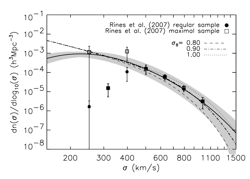
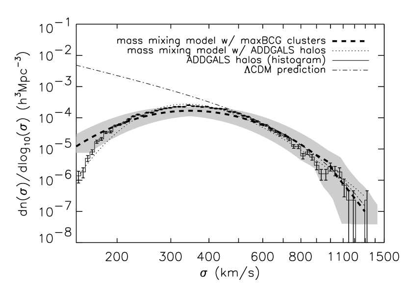
6. Dependence of the Velocity Dispersion on Secondary Parameters
In discussing the scatter model and the corrected velocity dispersion values, we assumed no other significant dependencies of the velocity dispersion on parameters besides N. We address this assumption here through a variety of theoretically and observationally motivated tests. In the same way that dark matter halos are primarily characterized by their mass, we would like to determine what parameters primarily characterize the velocity structure of the maxBCG clusters. By splitting the sample of clusters at a given N value on secondary parameters and measuring the velocity dispersion of these secondary stacks with the 2GAUSS method, we can test for any dependencies.
6.1. Redshift Evolution
The dependence of the velocity dispersion on redshift is shown in the right panel of Figure 12. We find a modest dependence, with higher redshift clusters having increased velocity dispersions over lower redshift clusters of the same richness. Following arguments given by Evrard et al. (2007), we can roughly estimate if the observed redshift dependence is due to evolution in the relationship.

Evrard et al. (2007) have found a robust relation between the velocity dispersion and mass of dark matter halos that is constant with redshift and has been tested with several simulation codes:
| (13) |
where is the dark matter velocity dispersion, km s-1 is the dimensionless Hubble parameter, and is the mass within a sphere of over density 200 times the critical density at redshift . Differentiating at fixed mass gives
| (14) |
This quantity can be computed exactly, but given the poor quality of our data when split into three times as many bins, a rough approximation which uses the median redshift of our sample is sufficient. At , , which gives . Over the redshift range of our sample, , so the expected change in is , assuming a constant velocity bias. This change is too small to account for the differences seen in Figure 12. Therefore we conclude that there must be evolution in the N richness measure. A fractional decrease in N of 30-40% from the middle redshift bin to the upper redshift bin is consistent with our results. Such an evolution is likely to be a combination of true evolution in the number of galaxies at fixed mass (e.g. Kravtsov et al. 2004; Zentner et al. 2005) and evolution in the definition of the richness estimator at fixed halo occupation. There is evidence from the evolution of richness in both the data (see also Koester et al. 2007a) and the mock catalogs, that the current definition of N does have mild evolution. It may however, be possible to use a slightly modified richness estimator which does not evolve at fixed mass. We do not explore this possibility further here, but note that velocity dispersion values will be useful in assessing the evolution of the N measure and attempts to correct for it.
We finally note that the observed evolution could have other explanations as well. Above redshift , the spectroscopic sample is dominated by LRGs. A relative velocity bias between galaxies of different colors and/or luminosities (e.g. Biviano et al. 1992) in clusters could potentially be the cause of the observed evolution.
6.2. Environmental Dependence and Local Density
Considerable attention has been devoted to the environmental dependence of the velocity dispersion in N-body simulations (e.g. Sheth & Diaferio 2001). It has been found that the velocity dispersion does depend on local density, but only because massive halos tend to occupy more dense environments (i.e. halo bias) and the velocity dispersion is strongly correlated with halo mass. No direct dependence of the velocity dispersion on the local density has been found (e.g. Sheth & Diaferio 2001).
In order to test this prediction, we construct four indicators of local density: N of closest cluster, the projected distance to the closest cluster, the total number of cluster members of any cluster within 5 Mpc and in redshift, and the total number of clusters within 5 Mpc and in redshift. This redshift cut is chosen to match twice the redshift cut used in the maxBCG percolation process to ensure that only clusters from one redshift slice on either side of the cluster under consideration are used.
We complete the test by comparing two binning schemes. First, we bin in N and then on the lower 25%, middle 50%, and upper 25% quantiles of the local density parameters within each N bin. This method should roughly account for the mass trend with cluster richness before comparing local environments. Second, we reverse the binning orders, using the lower 25%, middle 50%, and upper 25% quantiles of the N distribution in the second step. If there is in fact no dependence of the velocity dispersion on local density, except because massive halos tend to occupy more dense environments, then the relations in this binning scheme should be constant for a given N bin. Note however that if the halo occupation itself correlates with local density at fixed mass, then our test could be significantly biased.
Using this technique, we find little significant dependence of the velocity dispersion on any of our measures of local density. Figure 13 shows the results of this test for one of the parameters, the total number of clusters within 5 Mpc and in redshift. We have tested these results for fixed bins in N and the local density parameters, finding that they are robust. We applied these tests to the mock catalogs as well, producing similar results.

6.3. Multiple Bright Members and BCG -band Luminosity
It has been shown that clusters which have undergone recent mergers and show significant substructure are not virialized (e.g. Iguchi et al. 2005; Diaferio & Geller 1996) and that their velocity dispersions are increased above the expectation for their mass (e.g. Cortese et al. 2004; Halliday et al. 2004; Girardi et al. 2005). One might expect that a cluster with multiple bright members that resemble the BCG has undergone a recent merger or has significant substructure. However, it has also been shown that dark matter halos which form earlier at fixed mass have brighter, redder central subhalos (i.e. brighter, redder BCGs) and lower richness (e.g. Wechsler et al. 2006; Croton et al. 2007). Note that a brighter BCG at fixed mass for earlier forming halos likely corresponds to a larger magnitude difference between the BCG and the member galaxies.
We repeat the first binning scheme used above with the -band magnitude difference of the BCG and the next brightest cluster member as the secondary parameter. For each bin in N, the brightest member and BCG -band magnitude difference distribution is split by its lower 25%, middle 50%, and upper 25% quantiles. The naive expectation that clusters with more than one bright member might have undergone a recent merger or have significant substructure is not born out by the velocity dispersions, which show no significant increase. However, because the computations are done at fixed richness, it could be that late-forming halos, which have higher richness for their mass, also have higher velocity dispersions for their mass, because they merged recently, so that the two effects conspire to roughly cancel each other. Unfortunately, this hypothesis is difficult to test observationally.
One can similarly test for mass dependence of the clusters on the luminosity of the BCG alone. In the lower right panel of Figure 13, we plot the velocity dispersion of the clusters first binned in N and then in the absolute -band magnitude of the BCG using the lower 25%, middle 50%, and upper 25% quantiles within each N bin. We see dependence on this parameter: at fixed richness, clusters with more luminous BCGs have higher velocity dispersions. This same effect is observed in the stacked X-ray measurements of these same clusters by (Rykoff et al. 2007, in preparation); here, clusters with brighter BCGs have on average more X-ray emission. These observations indicate that BCG luminosity may contain additional information about cluster mass beyond that in N alone.
In the case of BCG -band luminosity, the expectd correlation mentioned above consistent with the observations, since early-forming halos would have brighter BCGs and lower richness, so that at fixed richness, halos with brighter BCGs tend to be more massive. However, for this explanation to be consistent with the previous hypothesis concerning the magnitude difference of the BCG and the next brightest cluster member, we must assume that whether or not a halo has formed through a major merger recently correlates more strongly with the magnitude difference of the BCG and the next brightest member galaxy, than with the BCG -band luminosity alone. In other words, we need to assume that the BCG -band luminosity is not indicative of a recent major merger (which would cause the velocity dispersion to be overestimated at fixed mass), even though BCG -band luminosity correlates with formation time.
6.4. Cluster Concentration and Radial Dependence
Although we cannot measure the true mass concentration, we investigate the dependence of the velocity-dispersion richness relation on the galaxy concentration, measured here by the ratio of the number of cluster members (determined by the maxBCG cluster finder, not the number of pairs in the BGVCF) within 0.2 R200 to the number of members within R200. We see no dependence of the velocity dispersions on this parameter when the dependence on N is accounted for first. When one bins directly on this ratio, the velocity dispersion decreases with increasing concentration.
Finally, we investigate the dependence of the velocity dispersion on cluster radius. The scaling of with radius is measured in logarithmic bins of N. In general, the dispersion stays constant or decreases with radius. This is consistent with the results from previous studies (e.g. Rines et al. 2003; Rines & Diaferio 2006).
7. Connecting Velocity Dispersion to Mass
Using velocity measurements to probe cluster masses has a long history in astronomy; the virial theorem was the earliest tool used to determine cluster masses (e.g. Zwicky 1933, 1937; Smith 1936) and remains in use today (e.g. Girardi et al. 1998; Struble & Rood 1999; Rines et al. 2003, 2006; Rines & Diaferio 2006). Other methods for determining cluster masses, such as the projected mass estimator (a modified virial mass estimator) (e.g. Heisler et al. 1985; Rines et al. 2003; Rines & Diaferio 2006), the Jeans equation (e.g. Carlberg et al. 1997; Girardi et al. 1998; van der Marel et al. 2000; Biviano & Girardi 2003; Rines et al. 2003; Katgert et al. 2004), and the caustic method (Diaferio & Geller 1997; Diaferio 1999) have also been widely applied (e.g. Biviano & Girardi 2003; Rines et al. 2003, 2006; Diaferio et al. 2005; Rines & Diaferio 2006).
In order to connect the velocity-dispersion–richness relation to a mass–richness relation, we use the recent results of Evrard et al. (2007), who found a dark matter virial relation which appears to hold for all redshifts and a wide range of cosmologies. Evrard et al. (2007) used a suite of dissipationless simulations run with a range of simulation codes and resolutions to measure the velocity dispersion of dark matter particles at fixed mass. They find that the dark matter virial relation can be characterized as a power-law,
| (15) |
where km s-1 is the dimensionless Hubble parameter and is the mass within a sphere of over density 200 times the critical density at redshift z. The values of the fit parameters for the mean relation are found to be km s-1 and .
Evrard et al. (2007) additionally found that the scatter of velocity dispersion at fixed mass is well fit by a lognormal with a small scatter of only . However, the lognormal scatter in velocity dispersion at fixed mass does not directly relate to the scatter in mass at fixed velocity dispersion without assuming the shape of the halo mass function. In light of this difficulty, and the small scatter in the relation, we take the mean power-law relation given by Evrard et al. (2007) to be a completely deterministic relation.
As there is still substantial theoretical uncertainty in velocity bias, this will be a primary driver of the systematic error in the N-mass relationship. To avoid this uncertainty, we constrain a combination of velocity bias and mass as described below. Using the standard definition of velocity bias, where is the galaxy velocity dispersion and is the dark matter velocity dispersions. The virial relation for galaxy velocity dispersions then becomes
| (16) |
where the quantity parameterizes our lack of knowledge about velocity bias.
To use this relation with the maxBCG clusters, we calculate using the measured lognormal distribution of in each bin. The result is
| (17) | |||||
where and are given by the 2GAUSS fits for each N bin (i.e. equations 8 and 9 respectively). This value is then substituted for in equation 16. To account for the factor of , we repeat the 2GAUSS fits for each N bin, weighting each pair in the BGVCF by . The inclusion of this factor has a negligible effect on the observed evolution in §6.1. We include the correction for BCG bias by dividing our results by the average BCG bias factor raised to the power.
We apply this method first to the mock catalogs, to determine whether we recover an unbiased estimate of the mass–richness relation. In the left panel of Figure 14, we show the results of this procedure applied to the mock catalogs. The best-fit power-law is plotted as the solid curve. For comparison, the mean mass of a cluster in each N bin, computed as the mean mass of the halos matched to the clusters within the bin, is shown as the diamonds. We again see the slight over correction of the BCG bias correction. Because the mass is proportional to , the masses we measure in the mock catalogs are too low by . The dashed line in the left panel of Figure 14 shows the best-fit power-law relation between N and mass in the simulation, but with the normalization increased by 25%. Note that in the mock catalogs the velocity bias is defined to be unity, so that equation 16 should be exact with and .
The results for the maxBCG clusters are given in the right panel of Figure 14. The error bars include the theoretical uncertainties in both and . The theoretical uncertainties increase the error bars in our mass determinations by a fixed factor uniformly across each bin. The best-fit power-law for the mass-N relation is
and is shown as the solid line in the right panel of Figure 14. The dashed line shows the approximate effect of the BCG bias over correction by shifting the mass normalization up by 25%.

8. Conclusions and Future Prospects
In this paper we have presented new measurements of the BCG–galaxy velocity correlation function (BGVCF) for a sample of clusters identified from the SDSS with the maxBCG algorithm (Koester et al. 2007a, b). Through careful modeling of the shape of the BGVCF, we have measured the mean and scatter in velocity dispersion at fixed N. We find that the mean velocity dispersion at fixed N is well described by a power-law. The mean velocity dispersion increases from km s-1 for small groups to more than km s-1 for large clusters. The scatter in velocity dispersion at fixed N is at most % and falls to % as N increases. We test our methods on both the C4 cluster catalog and on mock catalogs. Although there may be a slight 5-10% downward bias in the mean velocity dispersion due to the corrections made for BCG bias, our method successfully recovers the true scatter in both of these data sets with little bias.
The method presented here for measuring the scatter depends on two assumptions: (1) the Gaussianity of the PVD histogram of a stacked set of clusters with similar velocity dispersion, and (2) the lognormal shape of the distribution of velocity dispersion at fixed richness. While the first assumption is valid in cluster samples produced by running the cluster finder on realistic mock catalogs, it is hard to directly test observationally. Simulations with galaxies based on resolved dark matter subhalos may clarify this issue. The second assumption is directly supported in the mock catalogs and by independent observations with the C4 catalog (Miller et al. 2005).
In addition to the measurement of the mean and scatter in the velocity-dispersion–richness relation, we explore the dependence of the velocity dispersion on parameters secondary to richness. The velocity dispersion seems to be affected significantly by the -band luminosity of the BCG. We also see velocity dispersion dependence on redshift and local density. While the correlation between N, velocity dispersion, and the BCG -band luminosity may be a true physical effect, we interpret the correlations of N and velocity dispersion with redshift and local density as unphysical, systematic effects of the maxBCG cluster finder. Ultimately, it may be that the best way to estimate cluster mass will be to use multiple observables in combination. By making the comparisons of different parameters and their dependence on velocity dispersion as done in this paper, we will be able to determine which observables correlate significantly with mass.
Our methods, in combination with weak lensing mass profiles measured for stacked maxBCG clusters (Sheldon et al. 2007, in preparation; Johnston et al. 2007, in preparation) and the radial phase-space information contained in the BGVCF, will allow for precise determinations of the velocity bias and the anisotropy of galaxy orbits in clusters. Precise measurements of these quantities will help to constrain current theoretical models of galaxy clustering and the velocity bias between dark matter and galaxies.
This work also demonstrates the feasibility of using our methods to measure the velocity dispersion function. The velocity dispersion function computed in this paper agrees with the results of Rines et al. (2006). However, given the current estimated systematic errors in our computation (due the selection function, photometric redshift errors, evolution in N, and the BCG bias correction), we are unable to reach any strong conclusions about the magnitude of . With this caveat, we do however see from Figure 11, that our results support a higher value of than the most recent CMB+LSS estimates (e.g. Spergel et al. 2006; Tegmark et al. 2006), as recently suggested by other analyses (e.g. Buote et al. 2006; Evrard et al. 2007; Rozo et al. 2007b). This conclusion is however degenerate with velocity bias. A velocity bias of approximately 1.1-1.2 could equally well explain our results.
The methods presented in this paper are a significant advancement for the use of optical cluster surveys to determine cosmology. Our method can fully characterize the velocity-dispersion–richness relation for any optical cluster survey with a large spectroscopic sample. Future redshift surveys with more galaxy redshifts will allow for more precise measurements of this scatter. Specifically, because the SDSS spectroscopy is mostly at or below , a higher redshift sample of spectroscopy would allow for further tests of any redshift dependence.
The measurement of the scatter in mass–observable relations is key to the measurement of cosmology from galaxy cluster surveys and self-calibration schemes (Lima & Hu 2004, 2005). Through adding an additional piece of observational information, the methods developed here will undoubtedly tighten constraints on and lift degeneracies in current estimates of cosmology.
Appendix A Group Weighted EM-Algorithm for 1-Dimensional Gaussian Mixtures with Equal Means
Here we present the modification of the standard EM-algorithm (Dempster et al. 1977) for
Gaussian mixture models that is used to fit the PVD histograms. It
has the advantage of weighting clusters (or groups) of points evenly
and fixing the the mean of each Gaussian to be equal. We also verify
that the algorithm works using simple numerical experiments. The
derivation and notation given here is that of Connolly et al. (2000) with our
changes noted appropriately.
Let index the number of Gaussians in the model, index the data points, and be the total number of data points in the group from which the data point is drawn. The statistical model for the entire set data set will be a sum of Gaussians plus a single constant background component. We differ from Connolly et al. (2000) by presenting the derivation of the algorithm with the background components included. Letting the Gaussian components be given as
| (A1) |
where is the common mean of all of the model components, is the standard deviation of the Gaussian, and the background component, , be given as
| (A2) |
where is the range of all of the data, , we can write the model as
| (A3) |
where the ’s are the weights for each model component and we
require that . This model is exactly that of
the standard EM-algorithm for Gaussian mixtures. The difference here will be in the structure of the latent variables.
Let be defined such that if the data point is in the Gaussian and otherwise. Now we can write the complete data log-likelihood as
| (A4) |
Now we perform the expectation step of the algorithm given the current parameter guesses, , computing
where is now weighted by cluster (or group) to give
| (A5) | |||||
and for the background
| (A6) | |||||
Now we compute the maximization step by maximizing over the parameters. Following Connolly et al. (2000), we first rewrite into a more manageable form and then maximize . Using the definition of our model and its components we have
| (A7) |
Letting
| (A8) |
and noting that , we get
where
| (A9) |
Now we rewrite as
| (A10) |
The maximum of subject to will be given by letting be given by equation A8 and the rest of the parameters by
| (A11) |
The primary differences between the derivation given here and that given by Connolly et al. (2000) are the re-weighted expectation values of , equations A5 & A6, and that the means of each of the Gaussian components are fixed to one value (i.e. equation A8). The cluster-weighting is encoded in the factor of in equations A5 and A6. Each cluster of points contributes an equal amount to the parameters of the mixture model, making the total model wighted by cluster, not by point.
In Figure 15, we plot the point-weighted histogram of data created from 5000 and 500 random draws from two Gaussians with dispersion 800 and 300 respectively along with the standard EM algorithm fit using 10 components. We also plot the cluster-weighted histogram of the same data fit with the EM algorithm derived above using 10 components (bold line). The shapes seen in the figure are expected. In the point-weighted case, the 5000 samples of the 800 width Gaussian dominate the PVD histogram so it appears to be Gaussian. However, in the cluster-weighted case, the two Gaussians of width 800 and 300 contribute equally. Thus we explicitly see the the non-Gaussianity in the histogram. In effect, by not weighting the histogram by cluster, one can “hide” non-Gaussianity statistically.

Appendix B Statistical Bias in the 2GAUSS Method
In this appendix, we describe the statistical bias correction we apply to the 2GAUSS method. Suppose we have random samples, , from a distribution, , characterized by a set of parameters, , so that we can write . A simple example would be a Gaussian characterized by its mean and variance. From these random samples, we can construct estimators, , of the moments of the distribution, . A well known example of an estimator of is the mean, . An estimator of the moment of a distribution is said to be unbiased if . In some cases the sampling distribution of an estimator can be computed exactly, so that bias can be computed and corrected for analytically.
Because the 2GAUSS method is rather complicated, instead of attempting to compute the bias analytically, we use a Monte Carlo method to estimate the bias. For each bin in N, we construct 10,000 Monte Carlo samples of the set of velocity separation values, , using the measured parameters and , the number of clusters in the bin, and the number of samples per cluster in the bin. Then we remeasure and for each Monte Carlo sample. From these 10,000 reestimations of and , we estimate the bias in the 2GAUSS method. We then use this bias to correct our measurements.
We note here that the Monte Carlo tests indicate that the estimations of and are correlated in a non-trivial way. The BAYMIX method would naturally account for these correlations in a transparent way. Alternatively, a different, unbiased procedure could be used to estimate and . One candidate method might be the use of Gauss-Hermite moments (van der Marel & Franx 1993). Given that we already have a well developed method to estimate and , we do not explore this possibility here. A detailed understanding of the correlations is beyond the scope of this work, but would be necessary for the use of these results to understand cosmology precisely.
References
- Abazajian et al. (2004) Abazajian, K. et al. 2004, AJ, 128, 502
- Abazajian et al. (2005) —. 2005, AJ, 129, 1755
- Adelman-McCarthy et al. (2006) Adelman-McCarthy, J. K. et al. 2006, ApJS, 162, 38
- Annis et al. (1999) Annis, J. et al. 1999, in Bulletin of the American Astronomical Society, 1391–+
- Bahcall et al. (2003) Bahcall, N. A. et al. 2003, ApJS, 148, 243
- Beers et al. (1990) Beers, T. C., Flynn, K., & Gebhardt, K. 1990, AJ, 100, 32
- Berlind et al. (2006) Berlind, A. A. et al. 2006, ApJS, 167, 1
- Biviano et al. (1992) Biviano, A., Girardi, M., Giuricin, G., Mardirossian, F., & Mezzetti, M. 1992, ApJ, 396, 35
- Biviano & Girardi (2003) Biviano, A., & Girardi, M. 2003, ApJ, 585, 205
- Blanton et al. (2003) Blanton, M. R. et al. 2003, ApJ, 592, 819
- Blanton et al. (2005) —. 2005, AJ, 129, 2562
- Böhringer et al. (2000) Böhringer, H. et al. 2000, ApJS, 129, 435
- Brainerd & Specian (2003) Brainerd, T. G., & Specian, M. A. 2003, ApJ, 593, L7
- Buote et al. (2006) Buote, D. A., Gastaldello, F., Humphrey, P. J., Zappacosta, L., Bullock, J. S., Brighenti, F., & Mathews, W. G. 2006, ApJ, in press, arXiv:astro-ph/0610135
- Caldwell (1987) Caldwell, N. 1987, AJ, 94, 1116
- Carlberg (1994) Carlberg, R. G. 1994, ApJ, 434, L51
- Carlberg et al. (1997) Carlberg, R. G., Yee, H. K. C., & Ellingson, E. 1997, ApJ, 478, 462
- Colín et al. (2000) Colín, P., Klypin, A. A., & Kravtsov, A. V. 2000, ApJ, 539, 561
- Connolly et al. (2000) Connolly, A. J., Genovese, C., Moore, A. W., Nichol, R. C., Schneider, J., & Wasserman, L. 2000, arXiv:astro-ph/0008187
- Conroy et al. (2005) Conroy, C. et al. 2005, ApJ, 635, 982
- Conroy et al. (2007) —. 2007, ApJ, 654, 153
- Conroy et al. (2006) Conroy, C., Wechsler, R. H., & Kravtsov, A. V. 2006, ApJ, 647, 201
- Cortese et al. (2004) Cortese, L., Gavazzi, G., Boselli, A., Iglesias-Paramo, J., & Carrasco, L. 2004, A&A, 425, 429
- Croton et al. (2007) Croton, D. J., Gao, L., & White, S. D. M. 2007, MNRAS, 374, 1303
- Dahle (2006) Dahle, H. 2006, ApJ, 653, 954
- Dempster et al. (1977) Dempster, A., Laird, N., & Rubin, D. 1977, J. Roy. Stat. Soc., 39, 1
- Diaferio (1999) Diaferio, A. 1999, MNRAS, 309, 610
- Diaferio & Geller (1996) Diaferio, A., & Geller, M. J. 1996, ApJ, 467, 19
- Diaferio & Geller (1997) —. 1997, ApJ, 481, 633
- Diaferio et al. (2005) Diaferio, A., Geller, M. J., & Rines, K. J. 2005, ApJ, 628, L97
- Diemand et al. (2004) Diemand, J., Moore, B., & Stadel, J. 2004, MNRAS, 352, 535
- Eisenstein et al. (2001) Eisenstein, D. J. et al. 2001, AJ, 122, 2267
- Evrard et al. (2007) Evrard, A. E. et al. 2007, ApJ, submitted
- Evrard et al. (2002) —. 2002, ApJ, 573, 7
- Faltenbacher & Diemand (2006) Faltenbacher, A., & Diemand, J. 2006, MNRAS, 369, 1698
- Faltenbacher et al. (2005) Faltenbacher, A., Kravtsov, A. V., Nagai, D., & Gottlöber, S. 2005, MNRAS, 358, 139
- Frenk et al. (1996) Frenk, C. S., Evrard, A. E., White, S. D. M., & Summers, F. J. 1996, ApJ, 472, 460
- Fukugita et al. (1996) Fukugita, M., Ichikawa, T., Gunn, J. E., Doi, M., Shimasaku, K., & Schneider, D. P. 1996, AJ, 111, 1748
- Gerke et al. (2005) Gerke, B. F. et al. 2005, ApJ, 625, 6
- Ghigna et al. (2000) Ghigna, S., Moore, B., Governato, F., Lake, G., Quinn, T., & Stadel, J. 2000, ApJ, 544, 616
- Girardi et al. (1993) Girardi, M., Biviano, A., Giuricin, G., Mardirossian, F., & Mezzetti, M. 1993, ApJ, 404, 38
- Girardi et al. (2005) Girardi, M., Demarco, R., Rosati, P., & Borgani, S. 2005, A&A, 442, 29
- Girardi et al. (1998) Girardi, M., Giuricin, G., Mardirossian, F., Mezzetti, M., & Boschin, W. 1998, ApJ, 505, 74
- Gladders & Yee (2000) Gladders, M. D., & Yee, H. K. C. 2000, AJ, 120, 2148
- Gladders & Yee (2005) —. 2005, ApJS, 157, 1
- Gladders et al. (2007) Gladders, M. D., Yee, H. K. C., Majumdar, S., Barrientos, L. F., Hoekstra, H., Hall, P. B., & Infante, L. 2007, ApJ, 655, 128
- Grego et al. (2000) Grego, L., Carlstrom, J. E., Joy, M. K., Reese, E. D., Holder, G. P., Patel, S., Cooray, A. R., & Holzapfel, W. L. 2000, ApJ, 539, 39
- Gunn et al. (1998) Gunn, J. E. et al. 1998, AJ, 116, 3040
- Halliday et al. (2004) Halliday, C. et al. 2004, A&A, 427, 397
- Hansen et al. (2005) Hansen, S. M., McKay, T. A., Wechsler, R. H., Annis, J., Sheldon, E. S., & Kimball, A. 2005, ApJ, 633, 122
- Heisler et al. (1985) Heisler, J., Tremaine, S., & Bahcall, J. N. 1985, ApJ, 298, 8
- Iguchi et al. (2005) Iguchi, O., Sota, Y., Tatekawa, T., Nakamichi, A., & Morikawa, M. 2005, Phys. Rev. E, 71, 016102
- Izenman (1991) Izenman, A. J. 1991, Journal of the American Statistical Association, 86, 205
- Jenkins et al. (2001) Jenkins, A., Frenk, C. S., White, S. D. M., Colberg, J. M., Cole, S., Evrard, A. E., Couchman, H. M. P., & Yoshida, N. 2001, MNRAS, 321, 372
- Johnston et al. (2007) Johnston, D. E., Sheldon, E. S., Tasitsiomi, A., Frieman, J. A., Wechsler, R. H., & McKay, T. A. 2007, ApJ, 656, 27
- Katgert et al. (2004) Katgert, P., Biviano, A., & Mazure, A. 2004, ApJ, 600, 657
- Koester et al. (2007a) Koester, B. P. et al. 2007a, ApJ, in press, arXiv:astro-ph/0701265
- Koester et al. (2007b) —. 2007b, ApJ, in press, arXiv:astro-ph/0701268
- Kravtsov et al. (2004) Kravtsov, A. V., Berlind, A. A., Wechsler, R. H., Klypin, A. A., Gottlöber, S., Allgood, B., & Primack, J. R. 2004, ApJ, 609, 35
- Lancaster et al. (2005) Lancaster, K. et al. 2005, MNRAS, 359, 16
- Levine et al. (2002) Levine, E. S., Schulz, A. E., & White, M. 2002, ApJ, 577, 569
- Lima & Hu (2004) Lima, M., & Hu, W. 2004, Phys. Rev. D, 70, 043504
- Lima & Hu (2005) —. 2005, Phys. Rev. D, 72, 043006
- Mazure et al. (1996) Mazure, A. et al. 1996, A&A, 310, 31
- McKay et al. (2002) McKay, T. A. et al. 2002, ApJ, 571, L85
- Miller et al. (2005) Miller, C. J. et al. 2005, AJ, 130, 968
- Navarro et al. (1997) Navarro, J. F., Frenk, C. S., & White, S. D. M. 1997, ApJ, 490, 493
- Popesso et al. (2004) Popesso, P., Boehringer, H., & Voges, W. 2004, arXiv:astro-ph/0403357
- Prada et al. (2003) Prada, F. et al. 2003, ApJ, 598, 260
- Rines & Diaferio (2006) Rines, K., & Diaferio, A. 2006, AJ, 132, 1275
- Rines et al. (2006) Rines, K., Diaferio, A., & Natarajan, P. 2006, ApJ, in press, arXiv:astro-ph/0606545
- Rines et al. (2003) Rines, K., Geller, M. J., Kurtz, M. J., & Diaferio, A. 2003, AJ, 126, 2152
- Rosati et al. (1998) Rosati, P., della Ceca, R., Norman, C., & Giacconi, R. 1998, ApJ, 492, L21+
- Rozo et al. (2007a) Rozo, E., Wechsler, R. H., Koester, B. P., Evrard, A. E., & McKay, T. A. 2007a, ApJ, submitted, astro-ph/0703574
- Rozo et al. (2007b) Rozo, E. et al. 2007b, ApJ, submitted, astro-ph/0703571
- Sheth (1996) Sheth, R. K. 1996, MNRAS, 279, 1310
- Sheth et al. (2003) Sheth, R. K. et al. 2003, ApJ, 594, 225
- Sheth & Diaferio (2001) Sheth, R. K., & Diaferio, A. 2001, MNRAS, 322, 901
- Smith et al. (2002) Smith, J. A. et al. 2002, AJ, 123, 2121
- Smith (1936) Smith, S. 1936, ApJ, 83, 23
- Spergel et al. (2006) Spergel, D. N. et al. 2006, ApJ, in press, arXiv:astro-ph/0603449
- Springel et al. (2005) Springel, V. et al. 2005, Nature, 435, 629
- Stanek et al. (2006) Stanek, R., Evrard, A. E., Böhringer, H., Schuecker, P., & Nord, B. 2006, ApJ, 648, 956
- Strauss et al. (2002) Strauss, M. A. et al. 2002, AJ, 124, 1810
- Struble & Rood (1999) Struble, M. F., & Rood, H. J. 1999, ApJS, 125, 35
- Tasitsiomi et al. (2004) Tasitsiomi, A., Kravtsov, A. V., Wechsler, R. H., & Primack, J. R. 2004, ApJ, 614, 533
- Tegmark et al. (2006) Tegmark, M. et al. 2006, Phys. Rev. D, 74, 123507
- van den Bosch et al. (2004) van den Bosch, F. C., Norberg, P., Mo, H. J., & Yang, X. 2004, MNRAS, 352, 1302
- van den Bosch et al. (2005) van den Bosch, F. C., Weinmann, S. M., Yang, X., Mo, H. J., Li, C., & Jing, Y. P. 2005, MNRAS, 361, 1203
- van der Marel & Franx (1993) van der Marel, R. P., & Franx, M. 1993, ApJ, 407, 525
- van der Marel et al. (2000) van der Marel, R. P., Magorrian, J., Carlberg, R. G., Yee, H. K. C., & Ellingson, E. 2000, AJ, 119, 2038
- Warren (1994) Warren, M. S. 1994, PhD thesis, AA(California Univ., Santa Barbara, CA.)
- Wasserman et al. (2001) Wasserman, L. et al. 2001, arXiv:astro-ph/0112050
- Wechsler et al. (2006) Wechsler, R. H., Zentner, A. R., Bullock, J. S., Kravtsov, A. V., & Allgood, B. 2006, ApJ, 652, 71
- Wittman et al. (2006) Wittman, D., Dell’Antonio, I. P., Hughes, J. P., Margoniner, V. E., Tyson, J. A., Cohen, J. G., & Norman, D. 2006, ApJ, 643, 128
- Wojtak et al. (2006) Wojtak, R., Lokas, E. L., Mamon, G. A., Gottloeber, S., Prada, F., & Moles, M. 2006, A&A, in press, arXiv:astro-ph/0606579
- York et al. (2000) York, D. G. et al. 2000, AJ, 120, 1579
- Zehavi et al. (2005) Zehavi, I. et al. 2005, ApJ, 630, 1
- Zentner et al. (2005) Zentner, A. R., Berlind, A. A., Bullock, J. S., Kravtsov, A. V., & Wechsler, R. H. 2005, ApJ, 624, 505
- Zwicky (1933) Zwicky, F. 1933, Helvetica Physica Acta, 6, 110
- Zwicky (1937) —. 1937, ApJ, 86, 217