Coarsening of “clouds” and dynamic scaling in a far-from-equilibrium model system

Abstract

A two-dimensional lattice gas of two species, driven in opposite directions by an external force, undergoes a jamming transition if the filling fraction is sufficiently high. Using Monte Carlo simulations, we investigate the growth of these jams (“clouds”), as the system approaches a non-equilibrium steady state from a disordered initial state. We monitor the dynamic structure factor $S(k_{x},k_{y};t)$ and find that the $k_{x}=0$ component exhibits dynamic scaling, of the form $S(0,k_{y};t)=t^{\beta}\tilde{S}(k_{y}t^{\alpha})$. Over a significant range of times, we observe excellent data collapse with $\alpha=1/2$ and $\beta=1$. The effects of varying filling fraction and driving force are discussed.

I Introduction

The study of phase separation and coarsening in systems undergoing continuous or first-order phase transitions has a long history in physics and materials science Langer ; Gunton ; Bray ; Puri . A model system, like an Ising lattice gas, or a real alloy, like a mixture of tin and lead, is prepared in a high-temperature state and then suddenly quenched below its co-existence curve. As the system phase separates, its properties are dominated by the morphology of growing single-phase domains. A particularly interesting feature of many phase-ordering systems is dynamic scaling: if space and time are appropriately rescaled, growing domains at different times are found to be statistically self-similar, and the characteristic domain size, $R(t)$, grows as a power of time, $t^{\alpha}$. More detailed information is contained in the equal-time two-point correlation function, or equivalently, the structure factor, which are generalized homogeneous functions of space and time. For systems evolving towards terminal equilibrium states, the domain growth exponent $\alpha$ and the scaling behavior of correlation functions are fundamentally well understood Bray .

The situation is very different for many-body systems evolving towards non-equilibrium steady states (NESS). Maintained far from equilibrium by some external force, for example couplings to multiple energy or particle reservoirs, these systems carry nonzero fluxes. As a result, their stationary distributions lie outside the Boltzmann-Gibbs framework and are known only for a few special cases. Yet, nonequilibrium systems occur frequently in nature, particularly in many biological contexts. Not surprisingly, they display much richer behaviors than systems in thermal equilibrium SZ ; Mukamel , including a variety of pattern forming instabilities and first-order phase transitions, controlled by the external drive rather than a temperature variable. However, rather little is known about coarsening phenomena in such systems. Given that the underlying dynamics violates a very fundamental symmetry of equilibrium systems, namely, detailed balance, it is not immediately obvious whether features such as dynamic scaling or power law growth will persist when systems evolve towards terminal states which fall into the NESS class.

As a first step towards a better understanding of coarsening in such systems, it is instructive to investigate a few simple models, in the hope that these will generate insights from which a more general theory can be built. Looking for candidates which fall into the NESS class, which are well characterized in other sectors of their phase diagram and exhibit coarsening in some parameter regime, we are naturally led to driven diffusive systems KLS ; SZ . These systems involve one, or several, species of particles, diffusing on a lattice subject to a differential bias and short-range interactions. Both the prototype, first introduced KLS as a deceptively trivial modification of the Ising lattice gas, and its variants display many surprising and counterintuitive phenomena SZ . A particularly interesting modification involves models with two particle species driven in opposite directions Hwang ; Vilfan ; Thies1 where “jamming” transitions emerge from biased diffusion alone.

Let us very briefly survey earlier studies of domain growth and dynamic scaling in driven diffusive systems. The prototype model, an Ising-like lattice gas in which the particles are “charged” and driven by an external “electric” field $E$, sustains a nontrivial particle current on a fully periodic lattice. Still, the order-disorder transition of the undriven system survives, separating a disordered phase from a low-temperature phase which phase-separates into high- and low-density strips, aligned with the drive. If the system is quenched from a typical high-temperature state into the phase-separated sector of the phase diagram, coarsening of single-phase domains occurs ALLZ ; LKM . Some interesting morphological discrepancies between simulation data and results from a continuum theory ALLZ were eventually resolved RY . Turning to two-species models, the onset of jamming separates a homogeneous, high-current phase from a spatially inhomogeneous, low-current phase. As in the single species case, the jams take the form of strips of high particle density, but these are now aligned transverse to the field direction. At the late stages of the approach to the steady state, the system typically exhibits several strips which coarsen until only a single strip remains in the long-time limit.

Earlier work on dynamic properties has mostly focused on these late stages. Since the strips are (on average) uniform in the transverse direction, they are quite well described by a set of mean-field equations, in one space dimension and time Vilfan ; Thies2 . If the excluded volume constraint is enforced rigorously, so that the particles are not allowed to swap places, the strips coarsen logarithmically slowly KR ; Thies2 . Another group of studies investigates systems where the microscopic dynamics is already restricted to one God ; Gro , or quasi-one Met ; Geo , dimension. For interesting behavior to occur, particle-particle (“charge”) exchanges must be permitted, albeit with a small rate, compared to particle-hole exchanges. Provided the model parameters are chosen appropriately, compact particle clusters form easily, and coarsen until one a single large cluster remains. By virtue of the charge exchange process, power law growth dominates here.

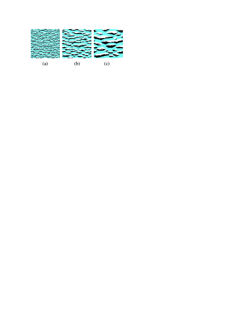
Figure 1: Snapshots of an $800\times 800$ system, at (a) $t=1024$, (b) $4096$, and (c) $16384$, in units of MCS. $E=10$. Positive (negative) particles are black (white); holes are blue.

In this article, we present the first study of fully two-dimensional coarsening in a two-species model with a strict excluded volume constraint. Starting from an initially disordered configuration, the system parameters (density, bias) are chosen so as to favor a jammed phase. Almost immediately, small “clouds” (Fig. 1) of locally jammed particles form. The larger clouds then grow, at the expense of the smaller ones, until a large cloud percolates along the transverse direction, forming a strip. Eventually, several strips emerge and compete with one another, on much slower time scales. We focus on the multi-cloud regime, long before the late-stage strip coarsening regime sets in. We monitor the equal-time structure factor $S(\mathbf{k},t)$, as a function of wave vector $\mathbf{k}$ and time $t$, averaged over initial conditions and system histories. A range of system sizes, densities, and $E$-values are studied. Since the field selects a specific direction, the $y$-axis, it is not surprising that the structure factors are anisotropic, in $k_{x}$ and $k_{y}$. More remarkably, we find that the system exhibits good dynamic scaling in $k_{y}$ and $t$, provided $k_{x}$ is fixed at $k_{x}=0$. Assuming the scaling form $S(0,k_{y},t)=t^{\beta}\tilde{S}(k_{y}/t^{\alpha})$, the scaling exponents are found to be $\alpha=1/2$ and $\beta=1$. For nonzero values of $k_{x}$, or in the full $(\mathbf{k},t)$ domain, we have not been able to achieve good data collapse.

This paper is organized as follows. We first present the model, a set of diagnostic observables, and some technical details of the simulations. Next, we discuss our simulation results and evidence for dynamic scaling. We conclude with some comments and open questions.

II The model and its observables

Our model is defined on a two-dimensional square lattice of size $L_{x}\times$ $L_{y}$ with fully periodic boundary conditions. Two species of particles, referred to as “positive” and “negative”, reside on the sites of the lattice, subject to an excluded volume constraint. Hence, a given configuration of the system can be labelled by a set of occupation variables, $\sigma(\mathbf{r})$, taking the values $0$, $+1$, and $-1$ if the site $\mathbf{r}=(x,y)$ is empty or occupied by a positive or negative particle, respectively. The particles experience no interactions, apart from respecting an excluded volume constraint. For simplicity, we restrict ourselves to systems which are neutral: $\sum_{\mathbf{r}}\sigma(\mathbf{r})=0$. For later reference, we also define the particle (as opposed to charge) occupation $n(\mathbf{r})$ via

$$n(\mathbf{r})=\left|\sigma(\mathbf{r})\right|$$ (1)

so that the total particle density (“mass”) $m$ is given by $m=\left(L_{x}L_{y}\right)^{-1}\sum_{\mathbf{r}}n(\mathbf{r})$.

In the absence of the driving force, the particles perform simple diffusion, i.e., jump with equal probability to a randomly selected nearest-neighbor site, provided it is unoccupied. As a result, there is no net current (of either mass or “charge”) through the system, and the steady state is spatially uniform. In contrast, an “electric” field, applied in the positive $y$-direction, biases positive and negative particles in opposite directions. In our simulations, a bond is selected at random and the occupancies of the two associated sites are checked. If the bond carries a particle-hole pair, an exchange will always be made if this results in a positive (negative) particle moving in the transverse or positive (negative) $y$-direction; otherwise, the exchange is attempted with rate $\exp(-E)$. Clearly, this dynamics is translation-invariant and invariant under charge-parity transformation ($\sigma\rightarrow-\sigma$, $y\rightarrow-y$). We use a random sequential dynamics, with one Monte Carlo step (MCS) corresponding to $L_{x}\times L_{y}$ update attempts. All runs start from a random initial condition.

The system sizes studied ranged from $100\times 100$ to $3200\times 3200$. The density varied from $m=0.3$ to $m=0.7$. We also considered different values for the probability for a particle to move backwards. Our reference system, for which the largest data set was collected, is an $800\times 800$ lattice, with $m=0.5$ and $E=10$. The latter gives a probability of $4.5\times 10^{-5}$ for backward jumps which is zero for all practical purposes. Runs lasted at least $8196=2^{13}$ MCS, and data are typically averaged over $1,000$ runs, unless stated otherwise. Time is measured in MCS.

The final stationary state of the system is well understood. For sufficiently large particle density $m$ and field $E$, the system displays a single strip of particles, transverse to the field direction Hwang . In that fashion, translational symmetry is spontaneously broken. The strip itself is charge-segregated, with positive (negative) particles occupying sites with lower (higher) $y$-coordinates. The interior interface (separating positive from negative particles) is glassy, due to the absence of any charge exchanges. In contrast, the exterior interfaces (separating particles from holes) is quite smooth, since its fluctuations are controlled by suppressed particle moves, i.e., by the parameter $\exp(-E)$. This parameter also controls the density of particles in the remainder of the system, reminiscent of a gas-liquid interface under gravity. Due to the periodic boundary conditions, however, a small current flows, even in the jammed phase, limited by $\exp(-EL_{y})$. A simple mean-field theory allows us to compute average density profiles, currents, and the phase diagram, in good agreement with the simulations Hwang ; Vilfan ; Thies1 .

In the following, we will always choose system parameters such that the system evolves towards an inhomogeneous, jammed final state. Starting from a random initial disordered configuration, small jams of positive and negative particles form very rapidly, due to local density fluctuations. Some of these, typically the larger ones, will collect more particles and grow, while others shrink and dissolve, as illustrated in Fig. 1. We refer to this stage as the coarsening of clouds, or clusters. Eventually, first one and then several of the largest clouds will span the lattice in the transverse direction, and the evolution is no longer dominated by the coarsening of well-separated clouds. Now, multiple strips compete for particles until only a single one remains, and the system has reached its steady state.

In this study, the characteristic shapes and separations of the clusters are of interest. Thanks to translational invariance, a suitable observable is the equal-time structure factor, defined through the Fourier transform of the local occupation,

$$\vskip 3.0pt plus 1.0pt minus 1.0ptS(k_{x},k_{y};t)=\frac{1}{L_{x}L_{y}}\left\langle\left|\sum_{x=0}^{L_{x}}\sum_{y=0}^{L_{y}}n(x,y;t)e^{i(k_{x}x+k_{y}y)}\right|^{2}\right\rangle$$ (2)

where $k_{x}=2\pi l/L_{x}$, $l=0,1,...,L_{x}-1$, and $k_{y}=2\pi j/L_{y}$, $j=0,1,...,L_{y}-1$. Here, $n(x,y;t)$ denotes the local occupation of site $(x,y)$ at Monte Carlo time $t$. The average $\left\langle...\right\rangle$ is taken over multiple runs, using configurations recorded at the same Monte Carlo time. All initial conditions are random.

Let us first establish a few properties of this structure factor. The value at the origin is easily found:

$$S(0,0)=\,\frac{1}{L_{x}L_{y}}<|\sum_{x,y}n(x,y)|^{2}>\,=m^{2}L_{x}L_{y}$$ (3)

Further, $S$ is related to the two-point correlation function, $G(x,y)\equiv\left\langle n(x,y;t)n(0,0;t)\right\rangle$, via

$$S(k_{x},k_{y};t)=\sum_{x,y}G(x,y)e^{i(k_{x}x+k_{y}y)}$$ (4)

which also provides us with the sum rule

$$\sum_{k_{x},k_{y}}S(k_{x},k_{y};t)=mL_{x}L_{y}$$ (5)

Finally, it is useful to evaluate $S$ for a few special cases, including the initial and final configurations. Since the time argument is inessential here, it will be suppressed for now. If the system is filled randomly with particles, at density $m$, the structure factor is easily found to be

$$S(k_{x},k_{y}) = m(1-m)\left[1+O(1/(L_{x}L_{y}))\right]$$ (6)

$$+ m^{2}\left(L_{x}L_{y}\right)\delta_{k_{x},0}\delta_{k_{y},0}$$

Clearly, $S(k_{x},k_{y})$ is uniform for all non-zero $\mathbf{k}\equiv(k_{x},k_{y})$.

For comparison, we also evaluate the structure factor for a perfectly ordered single strip which reflects the stationary state, modulo fluctuations:

$$S(k_{x},k_{y})=\frac{L_{x}}{L_{y}}\delta_{k_{x},0}\left[\frac{1-\cos\left(mk_{y}L_{y}\right)}{1-\cos k_{y}}\right]$$ (7)

These expressions provide a few benchmarks for the simulation data presented below.

III Simulation results and tests for dynamic scaling

III.1 Unscaled structure factors.

In this section, we first present Monte Carlo data for raw (unscaled) structure factors. We have collected data for a wide range of $\mathbf{k}$. Roughly speaking, the $\mathbf{k}$-value of the peak position reflects a characteristic spacing of the growing clusters, while the peak width carries information about fluctuations. For illustration purposes, we show two projections here, namely $S(0,k_{y};t)$ and $S(k_{x},0;t)$ (Fig. 2). Plotted vs $k_{y}$, the data for $S(0,k_{y};t)$ show a distinct maximum which moves towards smaller values of $k_{y}$ for later times. In contrast, $S(k_{x},0;t)$ is monotonically decreasing in $k_{x}$, for all $t$. A fuller picture can be gleaned from contour plots of $S(k_{x},k_{y};t)$ which indicate that, even for the earliest times considered ($t\leq 50$ MCS), the maximum of $S$ is found on the $k_{x}=0$ axis. As time progresses, the peak position shifts from larger values of $k_{y}$ to smaller ones, and the peak height increases. These findings suggest that, as the first clouds emerge from the fully disordered initial configurations, they quickly develop a characteristic length scale in the field direction, but remain disordered in the transverse direction.

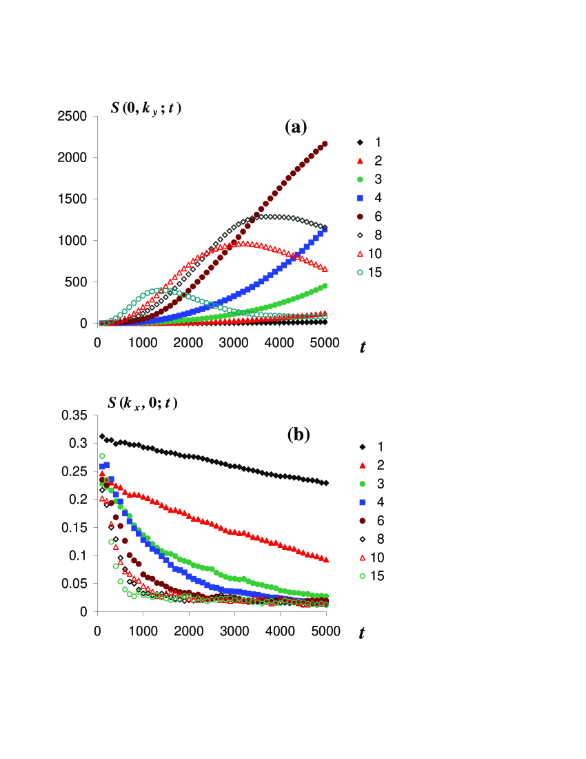
Figure 2: Unscaled structure factors $S(0,k_{y};t)$ (a) and $S(k_{x},0;t)$ (b) for an $800\times 800$ system, at $E=10$. The different curves correspond to different values of $j$ (top) and $l$ (bottom), specified in the legend. The notation is that of Eq. (2). Time is given in units of MCS.

III.2 Scaled structure factors

Snapshots of typical configurations at different times (Fig. 1) show clusters of particles (“clouds”) which grow in both the parallel and the transverse directions. If a simple rescaling of system size renders configurations, recorded at different times, statistically similar, we can hope for dynamic scaling, as illustrated by Fig. 3. After an appropriate rescaling of Figs. 1b and c, Fig. 1c is plotted inside Fig. 1b which is plotted inside Fig. 1a. One has to take a very careful look, if one wants to discern the internal boundaries (discontinuities) between the three pictures. This illustrates - at a simple visual level - how closely they resemble one another, after rescaling. However, our visual ability to detect scaling is easily deceived and provides, at best, the motivation for a more quantitative study.

Figure 3: Scaled configurations from Fig. 1. See text for details.

A quantitative test of dynamic scaling requires a careful analysis of the structure factors. Assuming that characteristic lengths in both directions increase as powers of time, but with possibly different exponents due to the anisotropy induced by the field, we first seek dynamic scaling in the form

$$S(k_{x},k_{y};t)\sim t^{\beta}f(k_{x}t^{\alpha_{1}},k_{y}t^{\alpha_{2}})$$ (8)

where the $\sim$ indicates that we should expect this form to hold only for certain ranges of time and wavevector. The sum rule, Eq. (5), immediately leads to the exponent identity

$$\alpha_{1}+\alpha_{2}=\beta$$ (9)

If dynamic scaling holds, one should be able to determine a set of scaling exponents in such a way that structure factor data for different times and wavevectors collapse onto a single curve if plotted according to Eq. (8). However, we have not been able to achieve satisfactory data collapse for this general form. Once again this suggests that there are no characteristic transverse length scales, associated with this growth process. It also illustrates that merely visual tests of scaling, such as Fig. 3, must be treated with some caution.

Turning to the remnant structures in $S(0,k_{y};t)$, the data in Fig. 2 show a sequence of curves of similar shapes, with the maximum shifting to smaller $k_{y}$ for later times. Even if the general form, Eq. (8), is not obeyed, we can explore the possibility of dynamic scaling in the reduced space $k_{x}=0$. In the remainder of this article, we focus on tests of

$$S(0,k_{y};t)\sim t^{\beta}f(0,k_{y}t^{\alpha})$$ (10)

Fig. 4 shows the scaling plot for a half-filled system for times ranging from $t=2^{9}=512$ to $t=2^{13}=8192$. We find excellent data collapse with the scaling exponents $\alpha=0.50\pm 0.02$ and $\beta=1.00\pm 0.02$. Much longer runs (with poorer statistics) show that the data continue to collapse well, until at least $t\sim O(10^{6})$. Our value for $\alpha$, the exponent controlling the characteristic spacing of domains, stands in stark contrast to its counterpart for conserved coarsening in equilibrium systems. There, it takes the value $1/3$, for a simple scalar density such as ours.

The scaling function exhibits Gaussian behavior near the maximum, and falls off as $z^{-3}$, where $z\equiv k_{y}t^{\alpha}$ is the scaling variable. This large $z$-behavior is highly reminiscent of the Porod tail Porod , well known in the theory of domain growth in equilibrium systems. There, it emerges from two essential features, namely, first, the presence of a single (isotropic) large length scale in the system, characterizing both the size and the separation of the coarsening domains, and second, the existence of microscopically sharp domain walls. Here, the situation is more complex. While we do observe sharp domain walls between our clouds and the surrounding (nearly) empty regions, our model is manifestly not isotropic. What complicates the issue further is the absence of a characteristic spacing in the direction transverse to the field. Clearly, a more careful study is required before the large $z$-behavior of our model can be traced directly to a simple Porod law. As for the small $z$-behavior, we hesitate to offer any conclusions. Certainly, it does not appear to follow the $k^{4}$ power law which would be expected for conserved coarsening in equilibrium systems Yeung .

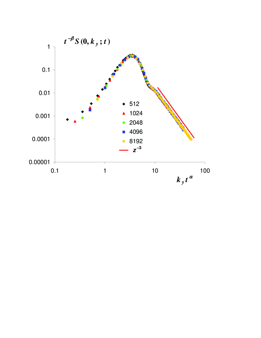
Figure 4: Scaling plot for $S(0,k_{y};t)$ for an $800\times 800$ system, at $m=0.5$ and $E=10$. Five different times, ranging from $t=512$ to $t=8192$, in units of MCS, are shown. $\alpha=1/2$ and $\beta=1$. The solid line denotes a $z^{-3}$ power law.

In the following, we probe the universality of the scaling exponents, as we change system parameters such as the particle density or the driving force. First, we consider the effect of system size. Since the scaling variable $z$ defines a characteristic length scale $\xi\propto t^{\alpha}$, it is natural to expect a breakdown of scaling when $\xi$ becomes of the order of $L$, or when considering times $t\gtrsim L^{1/\alpha}$. Indeed, scaling plots for a range of $L$, with $200\leq L\leq 566$ confirm this expectation very clearly. For example, in a $200\times 200$ system, the data for $t=10^{12}=4096$ already deviate noticeably from the scaling curve, whereas for $L=566$, such deviations are not observed until $t=2^{15}=32768$.

Next, we investigate the role of the overall particle density. For coarsening in conserved equilibrium systems, it is well known that the scaling function depends on volume fraction of the minority phase; however, the scaling exponents describing the structure factor remain unchanged Toral . Here, the situation is much more dramatic. Using the scaling exponents $\alpha=1/2$ and $\beta=1$, the data collapse for densities close to half-filling ($m=0.40$ and $0.55$) is still acceptable, but becomes progressively worse, for both larger ($m=0.70$) and smaller ($m=0.30$) densities. Better data collapse can still be achieved, but at the price of modifying the scaling exponents. Fig. 5 shows the scaled data, with appropriately adjusted values of $\alpha$ and $\beta$. It is natural to assume that these values reflect effective, rather than true asymptotic exponents. A better understanding of the scaling function would be necessary to disentangle its $m$-dependence from the overall scaling exponents.

We encounter a similar situation when considering the effect of the driving force, $E$. We find good data collapse, with $\alpha=1/2$ and $\beta=1$, as long as the rate for a particle to move against its preferred direction, set by $\exp(-E)$, remains small. Once $\exp(-E)$ becomes comparable to 0.2, deviations from scaling become noticeable. More work will be required to shed light on these preliminary observations.

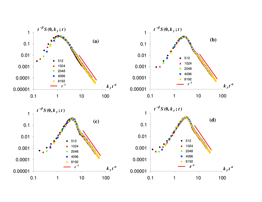
Figure 5: Scaling plots for $S(0,k_{y};t)$ for an $800\times 800$ system, at $E=10$. Four different densities are shown, and the scaling exponents are adjusted to give satisfactory data collapse: top left, $m=0.30$, $\alpha=0.46$, $\beta=0.98$; top right, $m=0.40$, $\alpha=0.50$, $\beta=1.00$; bottom left, $m=0.55$, $\alpha=0.50$, $\beta=1.00$; bottom right, $m=0.60$, $\alpha=0.44$, $\beta=0.95$. All errors are at most $5\%$. The solid lines denote $z^{-3}$ power laws.

IV Conclusions

To summarize, we have explored the possibility of dynamic scaling in a two-dimensional driven lattice gas, involving two species of particles. Positive and negative particles preferentially move in opposite directions and form small jams, due to an excluded volume constraint. Above a certain threshold density, these jams coarsen until a single strip of particles spans the system in the transverse direction. For an extended period of time, this coarsening process obeys dynamic scaling, provided we focus on characteristic length scales in the longitudinal direction. Monitoring a structure factor, $S(0,k_{y};t)$, we find very good data collapse provided $t^{-\beta}S$ is plotted vs $k_{y}t^{a}$. At and near half-filling ($m=0.5)$ and for large driving force, we find $\alpha=0.50\pm 0.02$ and $\beta=1.00\pm 0.02$. For smaller $E$ and densities further away from half-filling, we believe that the scaling function acquires a dependence on $m$ and $E$. We note that we can still achieve reasonable data collapse with the simple form given above, but only at the price of adjusting the exponents $\alpha$ and $\beta$. We believe that these effective exponents mask possibly significant modifications to the scaling function.

Naturally, a better analytic understanding of the exponents and of the scaling function would be desirable. It will be interesting to see what future studies in both simulations and analytics would reveal. The observation that $\alpha$ is essentially $1/2$ points towards a diffusive mechanism. Based on visual inspection alone, the clusters evolve by exchanging particles with one another. If this process is truly random - i.e., a cluster gains and loses particles with a fixed, constant rate, one should indeed expect to find a diffusive growth of characteristic length scales. Due to the drive, the particle exchange occurs predominantly between clusters which are nearest neighbors in the transverse direction; hardly any interactions occur between nearest neighbors in the transverse direction. This may explain the absence of any apparent structures in $k_{x}$. Work is in progress to analyze a well-established mean-field theory for this model, in the hope of gaining a better understanding of exponents and scaling function. If successful, it should also elucidate the deviations and similarities of our coarsening process with respect to those in equilibrium systems.

Acknowledgements. We have benefitted from discussions with K.E. Bassler and from the suggestions of a referee. This work is supported in part by the NSF through DMR-0414122.

References

- (1) J.S. Langer, Rev. Mod. Phys. 52, 1 (1980).
- (2) J.D. Gunton, M. San Miguel, and P.S. Sahni, in Phase Transitions and Critical Phenomena, Vol. 8, eds. C. Domb and J.L. Lebowitz (Academic, New York, 1983).
- (3) A.J. Bray, Adv. Phys. 43, 357 (1994).
- (4) S. Puri, Phase Transit. 77, 407 (2004).
- (5) B. Schmittmann and R.K.P. Zia, Statistical Mechanics of Driven Diffusive Systems, in: Phase Transitions and Critical Phenomena, Vol. 17, eds C. Domb and J.L. Lebowitz (Academic, New York, 1995).
- (6) D. Mukamel, in Soft and Fragile Matter: Nonequilibrium Metastability and Flow, eds. M.E. Cates and M.R. Evans (Institute of Physics Publishing, Bristol, 2000).
- (7) S. Katz, J. L. Lebowitz, and H. Spohn, Phys. Rev. B 28, 1655 (1983); and J. Stat. Phys. 34, 497 (1984).
- (8) B. Schmittmann, K. Hwang and R.K.P. Zia, Europhys. Lett. 19, 19 (1992).
- (9) I. Vilfan, R.K.P. Zia, and B. Schmittmann, Phys. Rev. Lett. 73, 2071 (1994).
- (10) M. Thies and B. Schmittmann, Phys. Rev E 61, 184 (2000).
- (11) F.J. Alexander, C.A. Laberge, J.L. Lebowitz, and R.K.P. Zia, J. Stat. Phys. 82, 1133 (1996).
- (12) E. Levine, Y. Kafri, and D. Mukamel, Phys. Rev. E 64, 026105 (2001).
- (13) A.D. Rutenberg and C. Yeung, Phys. Rev. E 60, 2710 (1999).
- (14) B. Schmittmann and M. Thies, Europhys. Lett. 57, 178 (2002).
- (15) J. Kertèsz and R. Ramaswamy, Europhys. Lett. 28, 617 (1994).
- (16) C. Godrèche, J. Phys. A 36, 6313 (2003).
- (17) S. Grosskinsky, G.M. Schütz, and H. Spohn, J. Stat. Phys. 113, 389 (2003).
- (18) J.T. Mettetal, B. Schmittmann, and R.K.P. Zia, Europhys. Lett. 58, 653 (2002).
- (19) I.T. Georgiev, B. Schmittmann and R.K.P. Zia, J. Phys. A 39, 3495 (2006).
- (20) G. Porod, Kolloid Z. 124, 83 (1951) and 125 51 (1952). See also, e.g., Ref. 3 for a thorough discussion.
- (21) C. Yeung, Phys. Rev. Lett. 61, 1135 (1988); H. Furukawa, J. Phys. Soc. Jpn. 58, 216 (1989) and Phys. Rev. B 40, 2341 (1989).
- (22) M. Tokuyama and Y. Enomoto, Physica A 204, 673 (1994); R. Toral, A. Chakrabarti, and J.D. Gunton, Physica A 213, 41 (1995).