Light Propagation on Quantum Curved Spacetime and Back reaction effects

Abstract

We study the electromagnetic field equations on an arbitrary quantum curved background in the semiclassical approximation of Loop Quantum Gravity. The effective interaction hamiltonian for the Maxwell and gravitational fields is obtained and the corresponding field equations, which can be expressed as a modified wave equation for the Maxwell potential, are derived. We use these results to analyze electromagnetic wave propagation on a quantum Robertson-Walker space time and show that Lorentz Invariance is not preserved. The formalism developed can be applied to the case where back reaction effects on the metric due to the electromagnetic field are taken into account, leading to non covariant field equations.

1 Introduction

There are several claims in the literature that one of the milestones of physics in the past century, namely Lorentz invariance, will no longer be true once a reliable quantum theory of gravity is achieved.

In its most simple and geometrical form, this invariance can be realized by introducing the Minkowski metric $\eta_{\mu\nu}$ as the “fixed backstage” to define distances or norms in special relativity. For example a photon is a particle whose 4-velocity $k^{\mu}$ has zero norm, i.e.

$$\eta_{\mu\nu}k^{\mu}k^{\nu}=0,$$

and the above equation is the geometrical casting of the invariance of the speed of light. What if light travels through cosmological distances? No problem, according to GR we simply replace the flat metric for the nontrivial metric $g_{\mu\nu}$ of the curved spacetime. Thus, Lorentz invariance in a local frame is generalized to covariance of the equations in an arbitrary frame. From this point of view the above equation is a scalar with respect to any coordinate transformation.

What if the classical metric $g_{\mu\nu}$ is replaced by a quantum operator $\widehat{g}_{\mu\nu}$? Here we face a problem, namely, the meaning of the resulting equation. A scalar equation can be obtained by taking an expectation value of the operator $\widehat{g}_{\mu\nu}$ with a suitable gravity state. If $k^{\mu}$ is a null vector with respect to $\langle\widehat{g}_{\mu\nu}\rangle$ for a particular state then in general it will not be a null vector with respect to a different gravity state. However, in this case one is not really breaking Lorentz invariance since taking expectation values with different states is like having classical metrics with different conformal structure and a vector is null with respect to both metrics if and only if the conformal structures are the same.

As a matter of fact it is difficult to imagine how to obtain non covariant observables if one is able to construct a theory with covariant field equations for the operators and the state vectors are invariant under the gauge transformations resulting from the diffeomorphism group.

However, to this day we do not have such a theory. Rather, the leading candidates for a quantum theory of gravity provide models for light propagation on a geometry constructed from a semiclassical quantum gravity state that break Lorentz invariance [1, 2]. The effects predicted by these models are within the detection limits of present technologies but the observed data severely compromise the validity of their results. Both loop quantum gravity and superstring theory predict a frequency dependent speed for photons propagating on a quantum spacetime. However, the approximately 3000 GRBs observed by BATSE and other space instruments showed that all the photons emitted by these bursts have the same flight time within the instruments sensitivity limits. Another prediction of loop quantum gravity concerns the rotation of the polarization direction for linearly polarized radiation but the observed synchrotron radiation for sources located at cosmological distances put severe restrictions on the phenomenological coupling constant of the model [3, 4]. It appears very likely that Lorentz invariance is preserved at the linearized approximation since the observed evidence points in this direction.

Upon a close look at the two models one finds possible resolutions to the conundrums. For example, the dispersion relation for photons obtained from the superstring model can be written as [5]

$$g_{\mu\nu}(k)k^{\mu}k^{\nu}=0,$$

that is, the metric of the spacetime depends on the energy of the photon. The equation is fully covariant and it does not say that different photons move with different speeds. It only says that, for the specific spacetime constructed with one photon interacting with gravity, the metric also depends on the energy of the photon. If one changes the energy of the photon one is also changing the spacetime and thus, it is “illegal” in GR to compare results coming from two different spacetimes. One could try to solve the problem of two photons with different energies interacting with a quantum gravity state but it appears very likely that if the problem is well set both photons should follow null geodesics as the observations suggest.

The loop quantum gravity model also admits a second look that offers an alternative explanation for the unobserved prediction. If we assume that the classical electromagnetic field is the 2-form $F_{\mu\nu}$, Lorentz invariance is preserved [6], whereas if we assume the canonical variables $(A_{\mu},-E^{\nu})$ can be regarded as classical objects, the invariance is broken. The problem arises from the relationship

$$E^{\mu}=g^{\mu\nu}E_{\nu}.$$

When the metric becomes a quantum operator $\widehat{g}^{\mu\nu}$ and one takes an expectation value of the above equation with a pure gravity state then both the covariant and contravariant versions of the electric field cannot be regarded as classical variables. If one assumes that the field of the l.h.s. is not affected by the gravity state one obtains non-lorentzian equations of motion. If, one the other hand, one assumes that the electric field of the r.h.s is transparent to the action of the expectation value then Lorentz invariance is preserved at a semiclassical approximation, i.e., neglecting back reaction effects. If the invariance is broken it must come from taking into account these back reaction effects.

The aim of this work is to study the propagation of light interacting with a semiclassical quantum gravity state when back reaction effects are included in this interaction. The goal is to see whether or not covariant equations of motion are obtained for this propagation. A more precise or technical meaning of this problem is given in Section 3 were it is defined and analyzed. However, in section 2 we address the propagation of photons on a non-flat semiclassical gravity state since these results are later used in the main section of this work. The derivations on Section 2 can also be used as a review of our previous work or as a toy model for photons propagating on a geometry given by semiclassical quantum gravity states that are peaked around a non trivial classical metric, as for example a Robertson Walker spacetime. Finally, in the Conclusions we summarize our work.

2 Propagation of electromagnetic radiation on a non-flat semiclassical geometry.

In this section we analyze the interaction of quantum gravity and Maxwell fields acting on quantum states that are a direct product of coherent states for the electromagnetic field and weave states for gravity. The non-trivial equations of motion that are obtained from such a scheme is called the semiclassical approximation of loop quantum gravity. A derivation of these equations follows

2.1 The effective interaction Hamiltonian in the semiclassical approximation

Assume an arbitrary background metric $g_{\mu\nu}$, and consider a 3+1 splitting of the spacetime by introducing a foliation of space-like hypersurfaces. We can set coordinates $(t,\vec{x})$ adapted to the foliation such that the lapse and shift $N$ and $N^{a}$ are $1$ and $0$ respectively (particular gauge choice). Let $q_{ab}$ be the induced 3-metric on the $\Sigma_{t}$ (corresponding to $t=const$) surface.

We will assume that there exists a geometric weave state $|\Delta\rangle$ on $\Sigma_{t}$ such that, given the classical metric $q_{ab}$, $\langle\Delta|\hat{q}_{ab}|\Delta\rangle=q_{ab}+\mathcal{O}\left(\frac{\ell_{P}}{\Delta}\right)$, where $\hat{q}_{ab}$ is the quantum operator associated to the metric tensor, $\ell_{P}$ is Planck’s length, and $\Delta$ is the typical length of the weave $|\Delta\rangle$. Such a state could be constructed, for example, by introducing random oriented Planck scale circular loops that form a graph adapted to the local geometry, and considering the product of the traces of the holonomies along these loops [7].

Now, if $E^{a}$ and $B^{a}$ are the electric and magnetic (purely spacial) fields on that background, the Hamiltonian density that couples these fields to gravity is given by

$$\mathcal{H}_{EB} = \frac{1}{2}\int_{\Sigma_{t}}d^{3}xq_{ab}\sqrt{det(q)}\left(E^{a}E^{b}+B^{a}B^{b}\right)$$ (1)

$$= \frac{1}{2}\int_{\Sigma_{t}}d^{3}xq_{ab}\hbox to0.0pt{\hss\lower 8.61108pt\hbox{$\widetilde{\hphantom{q_{ab}}}$}}(e^{a}e^{b}+b^{a}b^{b}),$$

where in the last line we have rewritten the Hamiltonian in terms of the vector densities $e^{a}$ and $b^{a}$ associated with $E^{a}$ and $B^{a}$, and $q_{ab}\hbox to0.0pt{\hss\lower 8.61108pt\hbox{$\widetilde{\hphantom{q_{ab}}}$}}$ is the 3-metric divided by its determinant. When the Hamiltonian is expressed in these variables, it is possible to implement Thiemann´s regularization procedure, which consists of a point splitting method where the operator associated with the metric divided by its determinant is written as the product of two operators $\hat{w}^{k}_{a}(\vec{x})$ (each one given by the commutator of the Ashtekar connection $A_{a}^{i}$ and the square root of the volume operator associated with $q_{ab}$, i.e. $\hat{w}^{k}_{a}(\vec{x})\equiv\left[A_{a}^{i}(\vec{x}),\sqrt{V(\vec{x})}\right]$ [8, 9]) evaluated at different points. In this way, the quantum operator corresponding to the electric part of the Hamiltonian density is

$$\mathcal{H}_{E}=\frac{1}{2}\int d^{3}x\int d^{3}y\delta_{kl}\hat{w}_{a}^{k}(\vec{x})\hat{w}_{b}^{l}(\vec{y})e^{a}(\vec{x})e^{b}(\vec{y})f_{\epsilon}(\vec{x}-\vec{y}),$$ (2)

and similar for the magnetic part. Here, $f_{\epsilon}(x-y)$ is a regularization function that tends to $\delta(x-y)$ as $\epsilon\rightarrow 0$. The next step in the regularization procedure consists of introducing a triangulation of the hypersurface $\Sigma_{t}$ into tetrahedra adapted to the graph associated with the weave state $|\Delta\rangle$ considered [8, 9].

The effective interaction Hamiltonian is then defined as the expectation value of the above operator in a semiclassical state that is given by the weave described before for the gravitational sector, and we will assume, in addition, that this state is close to a coherent state for the Maxwell sector, in such a way that, within our approximation, we can consider the electromagnetic field as a classical quantity. Under these assumptions, the effective Hamiltonian is given by

$$\mathcal{H}_{E} = \frac{1}{2}\int d^{3}x\int d^{3}y\delta_{kl}\langle\Delta|\hat{w}_{a}^{k}(\vec{x})\hat{w}_{b}^{l}(\vec{y})|\Delta\rangle e^{a}(\vec{x})e^{b}(\vec{y})f_{\epsilon}(\vec{x}-\vec{y})$$ (3)

$$= \frac{1}{2}\sum_{v_{i},v_{j}}\delta_{kl}\langle\Delta|\hat{w}_{a}^{k}(v_{i})\hat{w}_{b}^{l}(v_{j})|\Delta\rangle e^{a}(v_{i})e^{b}(v_{j}),$$

since, by construction, the operators $\hat{w}_{a}^{k}(\vec{x})$ only act at the vertices $v_{i}$ of the graph.

If we now assume that the variation scale of $e^{a}$ is large compared to the typical length of the weave state, we can expand it in a Taylor series around the central point $\vec{x}$ of the graph. Keeping only linear terms in $\ell_{P}$, and using the fact that the Hamiltonian is invariant under spacial rotations, we find that the electric part of the effective Hamiltonian is given, up to linear order, by:

$$\mathcal{H}_{Eeff}=\sqrt{det(q)}\left(\frac{1}{2}q^{ab}E_{a}E_{b}+\xi\ell_{P}\sqrt{det(q)}e^{abc}E_{a}\nabla_{b}E_{c}\right),$$ (4)

and similar for $B_{a}$. Here $\xi$ is a phenomenological coupling constant, $e^{abc}$ is the total antisymmetric tensor that represents the volume element of the classic 3-metric $q_{ab}$, $\nabla_{b}$ is the 3-dimensional covariant derivative consistent with $q_{ab}$ and we have expressed the Hamiltonian in the original variables (instead of vector densities). Also, we used the form $E_{a}$ and not the vector $E^{a}$ for reasons that will become clear in the following section.

2.2 The field equations

To derive the field equations from the above Hamiltonian we first need to determine the relationship between the electric and magnetic fields and the canonical variables. Let $A$ be the Maxwell connection and $F=dA$ the associated Maxwell 2-form. Then, the electric and magnetic fields that an observer with 4-velocity $t^{\mu}$ would measure are given by

$$E_{\mu} = F_{\mu\nu}t^{\nu},$$ (5)

$$B_{\mu} = -\frac{1}{2}\;e_{\mu\nu}{}^{\rho\delta}F_{\rho\delta}t^{\nu},$$ (6)

respectively, where $e_{\mu\nu\rho\delta}$ is the totally antisymmetric tensor associated to the volume element of $g_{\mu\nu}$ .

Note that, form the above expressions, both $E_{\mu}$ and $B_{\mu}$ are (as stated before) purely spacial vectors and that the definition (5) says that $E_{a}=-\partial_{t}A_{a}$ (we have chosen $A_{0}=0$ since we are only interested in wave propagation), which is independent of any background metric. On the other hand, if $\pi^{a}$ is the canonical momentum conjugated to $A_{a}$, Hamilton equations are

$$\partial_{t}A_{a} = \frac{\partial H}{\partial\pi^{a}},$$ (7)

$$\partial_{t}\pi^{a} = -\frac{\partial H}{\partial A_{a}}.$$ (8)

These expressions are consistent with (5) only if

$$E_{a}=-\frac{\partial H}{\partial\pi^{a}}=\frac{\partial H}{\partial E_{b}}\frac{\partial E_{b}}{\partial\pi^{a}},$$ (9)

which can be seen as a differential equation for $E_{a}(\pi^{b})$. By solving it we obtain the following relation between the electric field and the canonical momentum

$$\pi^{a}=-\sqrt{det(q)}\left(q^{ab}E_{b}+2\xi\ell_{P}\sqrt{det(q)}\;e^{abc}\;\nabla_{c}E_{b}\right),$$ (10)

or, symbolically

$$\pi^{a}=-H^{ab}E_{b},$$ (11)

where the “metric” operator $H^{ab}$ is given by

$$H^{ab}=\sqrt{det(q)}\left(q^{ab}+2\xi\ell_{P}\sqrt{det(q)}\;e^{abc}\;\nabla_{c}\right).$$ (12)

Note that eq. (11) is the semiclassical analogue of the relationship $\pi^{a}=-\sqrt{det(q)}q^{ab}E_{b}$.

Now, the second Hamilton equation, (7), leads to

$$\partial_{t}(H^{ab}E_{b})=H^{ab}e_{b}{}^{cd}\;\nabla_{c}B_{d}.$$ (13)

Introducing the definitions (5) and (6) of $E_{a}$ and $B_{a}$ in terms of the Maxwell potential we obtain the following expression

$$\nabla^{\mu}F_{\mu a}=2\xi\ell_{P}\partial_{t}[det(q)^{2}]H_{ad}e^{bcd}\nabla_{b}(F_{0c}),$$ (14)

where $\nabla^{\mu}$ is the 4-dimensional covariant derivative associated with the background metric $g$ and $H_{ab}$ is the inverse of $H^{ab}$. From this equation it becomes clear that the term on the left is the spatial component of a covariant expression and the term that breaks covariance appears in the right hand side. In particular, notice that for a stationary metric this term vanishes and we obtain a Lorentz invariant propagation.

2.3 Light propagation on a quantum flat FRW background

We can apply, as an example, the formalism developed in the previous section to the particular case of a flat Friedman-Robertson-Walker spacetime:

$$ds^{2}=-dt^{2}+a(t)^{2}(dx^{2}+dy^{2}+dz^{2}).$$ (15)

In this case, the metric operator acting on a vector $C_{a}$ is given by

$$H^{ab}C_{b}=\left(a(t)\delta^{ab}+2\xi\ell_{P}a(t)^{3}\epsilon^{abc}\partial_{c}\right)C_{b}$$ (16)

with $\epsilon_{abc}$ the Levi-Civita symbol, and the corresponding field equation (13) in the semiclassical approximation is

$$\partial_{t}(a(t)\vec{\hat{E}})=\nabla\times\vec{\hat{B}},$$ (17)

where we have adopted, for simplicity, vectorial notation and, for any given vector $\vec{C}$, the quantity $\vec{\hat{C}}$ is defined as:

$$\vec{\hat{C}}=\vec{C}-2\xi\ell_{P}a(t)^{2}\nabla\times\vec{C},$$ (18)

with $\nabla\times\vec{C}$ the usual 3-D curl in flat coordinates, i.e. $\left(\nabla\times\vec{C}\right)_{a}\equiv\epsilon_{a}{}^{bc}\partial_{b}C_{c}$. This is the only non trivial equation, since the other Hamilton equation (LABEL:H_1) gives no new information, it is just the definition of the electric field in terms of the potential. Note that in the above expression the indices are raised and lowered with the $\delta_{ab}$ 3-metric, and all the time dependence has been put explicitly.

On the other hand, the classical counterpart of eq (17) is

$$\partial_{t}(a(t)\vec{E})=\nabla\times\vec{B}.$$ (19)

There is another equation that relates $\vec{E}$ and $\vec{B}$, and it comes form the fact that, since $F=dA$, $dF=0$, which written in terms of the electric and magnetic fields defined by (5) and (6) reads:

$$\partial_{t}\vec{B}=-\frac{\dot{a}}{a}\vec{B}-\frac{\nabla\times\vec{E}}{a}$$ (20)

where $\dot{a}\equiv\frac{da}{dt}$. This expression holds both classically and in the semiclassical approximation we are analyzing.

Moreover, from the field equation (17) we can derive the wave equation satisfied by the Maxwell potential:

$$\partial_{t}(a\partial_{t}\vec{A})-\frac{\nabla^{2}\vec{A}}{a}=2\xi\ell_{P}\left(\partial_{t}(a^{3}\partial_{t}(\nabla\times\vec{A}))-a\nabla\times(\nabla^{2}\vec{A})\right),$$ (21)

while the classical covariant version is given by

$$\partial_{t}(a\partial_{t}\vec{A})-\frac{\nabla^{2}\vec{A}}{a}=0.$$ (22)

2.3.1 Plane Wave solutions

Consider, as a first step, light coming from a sufficiently close source. In that case we can take $a(t)\simeq const$ and the wave equation (21) reduces to

$$a\partial_{t}^{2}\vec{A}-\frac{\nabla^{2}\vec{A}}{a}=2\xi\ell_{P}a^{2}\nabla\times\left(a\partial_{t}^{2}\vec{A}-\frac{\nabla^{2}\vec{A}}{a}\right).$$ (23)

If we propose a plane wave solution of the form $\vec{A}=Re\left(\vec{A}_{0}e^{iS}\right)$ and introduce it in the above expression, we obtain the following dispersion relation for the wave vector $k_{\mu}=S_{,\;\mu}$

$$(-a^{2}k_{t}^{2}+k^{2})(1-2\xi\ell_{P}a^{2}k)=0,$$ (24)

where $k^{2}\equiv k_{x}^{2}+k_{y}^{2}+k_{z}^{2}$. We see, then, that the wave vector $k_{\mu}$ satisfies the usual dispersion relation $g^{\mu\nu}k_{\mu}k_{\nu}=0$.

Note that this result holds in the geometric approximation of wave propagation, since in that case we are dealing with the high frequency limit and we can neglect time derivatives of the expansion factor compared to time derivatives of the electromagnetic field.

If, on the other hand, we consider a source located at a cosmological distance, then we can not take $a(t)\simeq const$, we must take into account the terms containing time derivatives of $a$ and solve the complete wave equation (21) perturbatively since it does nos admit plane wave solutions with constant amplitude of the form proposed above. This is done more easily if we introduce the conformal time $\eta$, such that $\frac{d\eta}{dt}=a^{-1}$. Expressed in this conformal time, the FRW line element reads

$$ds^{2}=a(\eta)^{2}(-d\eta^{2}+dx^{2}+dy^{2}+dz^{2}),$$ (25)

and the wave equation (21) can be rewritten as

$$(1-2\xi\ell_{P}a^{2}\nabla\times)\square\vec{A}=4\xi\ell_{P}aa^{\prime}\nabla\times\vec{A}^{\prime},$$ (26)

where $\square\vec{A}\equiv\partial_{\eta}^{2}\vec{A}-\nabla^{2}\vec{A}$ and prime denotes derivative with respect to the conformal time $\eta$. Note that, in view of the conformal flatness of the metric (25), the associated classical wave equation is simply $\square\vec{A}=0$.

We will try to solve eq. (26) in a perturbative way, by proposing a solution of the form

$$\vec{A}=\vec{A}_{class}+\xi\ell_{P}\vec{\tilde{A}},$$ (27)

where $\vec{A}_{class}$ is the classical plane wave solution $\vec{A}_{class}=Re(\vec{A}_{0}e^{i(\omega\eta-\vec{k}\cdot\vec{x})})$, with $\omega^{2}=k^{2}$. Introducing the solution (27) into (26) and dropping terms of order $(\xi\ell_{P})^{2}$ we obtain the equation for $\vec{\tilde{A}}$:

$$\square\vec{\tilde{A}} = 4aa^{\prime}\nabla\times\vec{A}_{class}^{\prime}$$ (28)

$$= -4iaa^{\prime}\vec{k}\times\vec{A}_{class}^{\prime}$$

To find the final solution, we must say something about the expansion factor $a(t)$. Consider an Einstein-De Sitter model, that is, FRW universe dominated by matter. In this case the radius of the universe is given by $a(t)=\alpha t^{2/3}$, which, written in terms of the conformal time $\eta$ is

$$a(\eta)=\alpha\left(\frac{\alpha}{3}(\eta-\eta_{0})+t_{0}^{1/3}\right)^{2},$$ (29)

where the $0$ subindex denotes the moment $t_{0}$ of emission of the electromagnetic radiation, at which the expansion factor is assumed to have the value $a_{0}$ (this means that $\alpha=a_{0}t_{0}^{-2/3}$). Inserting this into (28) we can obtain the final solution:

$$\vec{A} = Re\left[e^{i(\omega\eta-\vec{k}\cdot\vec{x})}\left(\vec{A}_{0}+\xi\ell_{P}\alpha^{2}(\hat{n}\times\vec{A}_{0})(L(\omega,r)-L(\omega,r_{0}))\right)\right],$$ (30)

$$\equiv Re\left[e^{i(\omega\eta-\vec{k}\cdot\vec{x})}(\vec{A}_{0}+\xi\ell_{P}\vec{\Lambda}(\eta,\omega))\right],$$ (31)

where $\hat{n}=\frac{\vec{k}}{|\vec{k}|}$ and the function $L(\omega,r)$ is given by

$$L(\omega,r)=-\frac{\alpha^{3}r}{9\omega^{2}}+\frac{2\alpha r^{3}}{3}+i\left(\frac{\alpha^{2}r^{2}}{3\omega}-\omega r^{4}\right),$$ (32)

with $r=\frac{\alpha}{3}(\eta-\eta_{0})+t_{0}^{1/3}$ or, in terms of the comoving time, $r=t^{1/3}$. Note that we have imposed the condition that the solution coincides with the classical wave at the emission time $t_{0}$.

We see from eq. (30) that the final solution corresponds to a plane wave with the standard dispersion relation and hence with no modification on the propagation speed, but with a corrected amplitude vector due to quantum gravity effects. As we will see in the following, the interaction of the electromagnetic radiation with the quantum spacetime induces a frequency dependent correction on the polarization direction of the initial wave, while its amplitude is, within the linear approximation considered, not affected.

To see how this correction behaves, consider a normalized and linearly polarized initial wave. Introducing a unitary right handed basis $(\hat{e}_{1},\hat{e}_{2},\hat{n})$ and assuming that the initial Maxwell potential is polarized along the $\hat{e}_{1}$ direction, we obtain, by taking the real part of (30)

$$\vec{A} = [\hat{e}_{1}+\xi\ell_{P}\hat{e}_{2}Re(L(\omega,r)-L(\omega,r_{0}))]cos(\omega\eta-\vec{k}\cdot\vec{x})$$ (33)

$$-\xi\ell_{P}\hat{e}_{1}\alpha^{2}Im(L(\omega,r)-L(\omega,r_{0}))sin(\omega\eta-\vec{k}\cdot\vec{x}).$$

From this expression we can not conclude any quantitative results for the correction to the magnitude of the amplitude vector, since it is given by

$$|\vec{A}_{0}+\xi\ell_{P}\vec{\Lambda}(\eta,\omega)|=|\vec{A}_{0}|+\mathcal{O}((\xi\ell_{P})^{2})$$ (34)

and we have been dealing with the linear approximation only (and hence dropping quadratic terms in the whole calculation that lead to this equation). On the other hand, the angle of rotation $\theta$ of the polarization vector can be obtained, leading to

$$\tan(\theta)=\xi\ell_{P}a_{0}t_{0}^{-2/3}\sqrt{Im(L(\omega,r)-L(\omega,r_{0}))^{2}+Re(L(\omega,r)-L(\omega,r_{0}))^{2}}.$$ (35)

Here $\theta$ is measured from the initial polarization direction, and it is an increasing function of both $t$ and $\omega$. More precisely, from (35) it is possible to prove that the tangent of the polarization angle has, for a given frequency, a behavior where the dominant term is of the form $t^{4/3}$ (see fig 1), while for a fixed instant of time the angle grows linearly with the photon energy (fig 2). Notice that this result is different from the one obtained by Gambini and Pullin [2], where the dependence of the polarization angle was quadratic in the photon energy. Note, in addition, that the solution (30) does not show the birefringence effect predicted in [2], since in our formalism the propagation velocity does not depend on the frequency, nor on the polarization state of the wave.

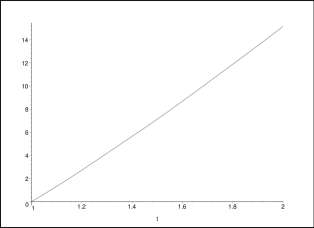
Figure 1: Tangent of the polarization angle as a function of the comoving time for a given photon energy, the behavior is of the form $\tan(\theta)\propto t^{4/3}$.

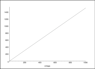
Figure 2: Tangent of the polarization angle as a function of the wave frequency for fixed $t$. The graph shows a linear behavior.

From the above considerations, we conclude that, through its flight time, the polarization direction of an electromagnetic wave will be rotating a frequency dependent angle $\theta(\omega)$. If a source emits a wave packet with a continuum spectrum, the high frequency photons will rotate a larger angle than the less energetic ones, the net result being a loss of linear polarization. The fact that we observe, nevertheless, light coming from cosmological sources with a high level of linear polarization is indicative that the effect, if present, is very small (some orders of magnitude below the sensitivity of the current instruments). Even more, we could use the available observational data to put a bound on the coupling constant $\xi$. Clearly, that bound would differ form the value obtained in [3, 4], since there a quadratic effect was assumed.

Just for completeness, suppose two photons are emitted simultaneously by a cosmological source located at distance $L$ with identical (linear) polarization state, and with wavelengths $\lambda_{1}$ and $\lambda_{2}$. Then, at the detection time their respective polarization directions would rotate in such a way that the difference between the corresponding angles would be given by

$$\Delta\theta=\xi_{rw}\ell_{P}\alpha\ (cL)^{4/3}\frac{c}{2\pi}\left(\frac{1}{\lambda_{1}}-\frac{1}{\lambda_{1}}\right).$$ (36)

To derive this expression we used (35) and, based on observational arguments, assumed $\theta\ll 1$ and therefore $\tan(\theta)\simeq\theta$. We have also considered only the leading terms in (35) since we are dealing with high frequencies and large distances. Hence, by using (36) we could, if we knew the constant $\alpha$, obtain the desired bound for $\xi$. However, we do not have enough information on the parameters of the universe to determine $\alpha$, which makes it extremely difficult to estimate that bound. On the other hand, for the curvature effects to be appreciable, we should have observations of sources at very high redshift, and we believe that, for the available data, the flat background approximation suffices and the bound obtained in [3, 4] is the most reliable.

Remarks:

• One thing worth mentioning is that, for non-stationary geometries, the assumption that it is possible to construct a weave state that is peaked at that specific metric for all times is a very strong one. If the 3-metric has, indeed, a non-trivial evolution, it is encoded in its conjugated variable (directly related to the extrinsic curvature of the hypersurface) and, since the weave does not satisfy the properties of a coherent sate (namely, that it approximates the configuration variable and its canonical conjugate), when one takes expectation value there is no control on $\partial_{t}\langle\hat{q}_{ab}\rangle$ and it could happen that $\langle\hat{q}_{ab}\rangle$ deviates significantly form the classical value after a short time.

• Even more, there are indications that for arbitrary curved spaces, the weave states might not be solutions of the Hamiltonian Constraint [7].  Thus, if the weave states cannot be considered physical, the results showed in this section may not reflect the real propagation of light on a semiclassical FRW spacetime, assuming of course one can find a suitable definition of semiclassical states.
  

• Note also that, in the derivation of the above equations, we have not taken into account the back reaction effects on the background geometry. It could happen that, even if the resulting equations locally preserve Lorentz invariance (for example if one only considers stationary backgrounds), this invariance could be broken if one considers the back reaction effect. This possibility is analyzed in the next section.

3 Lorentz Invariance and back reaction effects

In the previous sections we have considered wave propagation on a fixed background geometry, that is, we have neglected back reaction effects on the metric due to the electromagnetic field. However, Einstein’s equations couple gravity to any other forms of energy, in particular, with the Maxwell field, and we expect, therefore, that not only the quantum geometry will affect the propagation of electromagnetic waves, but also that the latter will modify, in turn, the spacetime itself. Here we will try to account for this back reaction effect by applying the formalism developed in section 3 to the full Einstein-Maxwell theory. To do so, we first have to analyze if it is reasonable to consider that we are within the assumptions made in that section, namely, that we have a classical metric expressed in the appropriate gauge, and a weave state that approximates that particular metric.

The classical equations that describe the Einstein-Maxwell theory are

$$G_{\mu\nu}=8\pi T_{\mu\nu},$$ (37)

$$\nabla^{\mu}F_{\mu\nu}=0,$$ (38)

where the Einstein tensor $G_{\mu\nu}$ is determined by the stess-energy tensor associated to the Maxwell field $F_{\mu\nu}$, that is

$$T_{\mu\nu}=\frac{1}{4\pi}\left(F_{\mu\sigma}F_{\nu}{}^{\sigma}-\frac{1}{4}g_{\mu\nu}F_{\delta\rho}F^{\delta\rho}\right),$$ (39)

and $\nabla^{\mu}$ is the covariant derivative consistent with $g_{\mu\nu}$.

The idea is to solve this system of equations with an approximation scheme were at the zeroth order the electromagnetic field propagates on a flat background. In other words the deviation from flatness arises from the electromagnetic stress energy tensor.

As stated above, there are two things that need to be considered:

• that there is a classical metric solution of (37) written in the gauge where $g_{tt}=-1$ and $g_{ta}=0$ (that is, we introduce a foliation adapted to the time field $t^{\mu}$, such that the lapse and shift functions are $N=1$ and $N^{a}=0$ respectively), and

• that it is reasonable to assume that we can construct a semiclassical state $|\psi\rangle$ that approximates the 3-metric $q_{ab}$ induced in the spacial hypersurfaces of the above mentioned foliation, that is, such that $\langle\psi|{\hat{q}}_{ab}|\psi\rangle=q_{ab}$ plus corrections of order $\ell_{P}$.

If we are able to affirm these two statements, then we can assume that the field equation for the electromagnetic field, within the semiclassical approximation of LQG, is given by eq. (13), with $H^{ab}$ and $e_{abc}$ the ones corresponding to the 3-metric $q_{ab}$ associated to the solution of (37).

The classical metric

We have to solve the field equation (37), with $T_{\mu\nu}$ given by (39). Since by assumption the Maxwell field introduces a small perturbation to the Minkowski metric $\eta_{\mu\nu}$, we will assume that the electromagnetic tensor is given by $\epsilon F_{\mu\nu}$, with $\epsilon$ a small parameter that will allow us to solve the equations by means of a perturbation expansion. Then, the classical metric will be given by

$$g_{\mu\nu}=\eta_{\mu\nu}+\epsilon g^{(1)}_{\mu\nu}+\epsilon^{2}g^{(2)}_{\mu\nu}+...$$ (40)

Besides, we will set the data (in the initial surface) of $g^{(1)}_{\mu\nu}$, $g^{(2)}_{\mu\nu}$, etc, equal to zero, since we are interested in the case where there are no incoming gravitational waves, and all the perturbation is generated by the interaction with the Maxwell field.

If we introduce (40) into (37), and consider a similar perturbative expansion for the electromagnetic field (and hence for the stress-energy tensor) given by

$$F_{\mu\nu}=\epsilon(F^{(1)}_{\mu\nu}+\epsilon F^{(2)}_{\mu\nu}+...),$$ (41)

$$T_{\mu\nu}=\epsilon^{2}(T^{(2)}_{\mu\nu}+\epsilon T^{(3)}_{\mu\nu}+...),$$ (42)

we can solve the coupled equations order by order in a recursive way, such that each order is determined by the previous ones. In this work we will focus on the first non trivial corrections to the free fields.

The term of Equation (37) that corresponds to linear order in $\epsilon$ is simply

$$G^{(1)}_{\mu\nu} = 8\pi T^{(1)}_{\mu\nu}$$ (43)

$$= 0,$$ (44)

since, the first non zero term of the stress-energy tensor is of order $\epsilon^{2}$, and, hence, we get the familiar result form linearized gravity [11]

$$\partial^{\delta}\partial_{(\mu}\bar{g}^{(1)}_{\nu)\delta}-\frac{1}{2}\;\partial^{\delta}\partial_{\delta}\bar{g}^{(1)}_{\mu\nu}-\frac{1}{2}\;\eta_{\mu\nu}\;\partial^{\rho}\partial^{\delta}\bar{g}^{(1)}_{\rho\delta}=0,$$ (45)

where $\bar{g}^{(1)}_{\mu\nu}=g^{(1)}_{\mu\nu}-\frac{1}{2}\eta_{\mu\nu}g^{(1)}$ with $g^{(1)}=\eta^{\mu\nu}g^{(1)}_{\mu\nu}$. Of course the above equation reduces to the well known wave equation $\partial^{\delta}\partial_{\delta}\bar{g}^{(1)}_{\mu\nu}=0$ in the Lorentz gauge. We will not, however, consider that gauge but another one consistent with (13). We will go back to this issue later.

The only solution of eq. (45) is $g^{(1)}_{\mu\nu}=0$, since, as mentioned before, the data for this perturbation in the initial surface is zero. On the other hand, looking at the first order in $\epsilon$ of eq (38) we get

$$\partial^{\mu}F^{(1)}_{\mu\nu}=0,$$ (46)

which sates, as expected, that $F^{(1)}_{\mu\nu}$ is the free Maxwell field in flat background.

Hence, the non trivial correction for both the electromagnetic field and metric tensor are at least of order $\epsilon^{2}$. The field equation for $g^{(2)}_{\mu\nu}$ is, in analogy to (45),

$$\partial^{\delta}\partial_{(\mu}\bar{g}^{(2)}_{\nu)\delta}-\frac{1}{2}\;\partial^{\delta}\partial_{\delta}\bar{g}^{(2)}_{\mu\nu}-\frac{1}{2}\;\eta_{\mu\nu}\;\partial^{\rho}\partial^{\delta}\bar{g}^{(2)}_{\rho\delta}=8\pi T^{(2)}_{\mu\nu},$$ (47)

with

$$T^{(2)}_{\mu\nu}=\frac{1}{4\pi}\left(F^{(1)}_{\mu\sigma}F^{(1)}_{\nu}{}^{\sigma}-\frac{1}{4}\eta_{\mu\nu}F^{(1)}_{\delta\rho}F^{(1)\delta\rho}\right),$$ (48)

and where all the indices are raised and lowered with $\eta_{\mu\nu}$. The above expressions prove that the first correction to the metric due to back reaction effects is generated by the free Maxwell filed. We will write, for simplicity,

$$g_{\mu\nu}=\eta_{\mu\nu}+\epsilon^{2}\gamma_{\mu\nu}$$ (49)

with $\gamma_{\mu\nu}$ such that $\bar{\gamma}_{\mu\nu}$ is a solution of (47 ).

Now, the formalism developed in the previous section requires that the metric is written in coordinates in which it takes the form

$$ds^{2}=-dt^{2}+q_{ab}dx^{a}dx^{b}.$$ (50)

This can be easily done if we use the gauge freedom in eq (47) that corresponds, precisely, to a coordinate choice. It is well known that, under the transformation $x^{\mu}\mapsto x^{\mu}+\epsilon\;\xi^{\mu}$, the perturbation changes according to $\gamma_{\mu\nu}\mapsto\gamma_{\mu\nu}+\partial_{\mu}\xi_{\nu}+\partial_{\nu}\xi_{\mu}$. In order to satisfy (50), the gauge choice must be such that $\gamma_{t\nu}=0$, which gives the four necessary conditions to fix the transformation generator $\xi^{\mu}$, namely

$$\partial_{t}\xi_{\nu}+\partial_{\nu}\xi_{t}=-\gamma_{t\nu}.$$ (51)

Hence, it is always possible to express the metric tensor in the form (50), and, in that particular gauge, $\gamma_{\mu\nu}$ has only spacial components.

To obtain the corrections to the electromagnetic field due to back reaction effects, we insert the solution (49) in the Maxwell equation $\nabla^{\mu}F_{\mu\nu}=0$. By doing so, we obtain

$$\partial^{\mu}F^{(2)}_{\mu\nu} = 0,$$ (52)

$$\partial^{\mu}F^{(3)}_{\mu\nu} = \gamma^{\mu\sigma}\partial_{\sigma}F^{(1)}_{\mu\nu}+\eta^{\mu\sigma}\left(\Gamma^{(2)\delta}_{\mu\sigma}F^{(1)}_{\delta\nu}+\Gamma^{(2)\delta}_{\nu\sigma}F^{(1)}_{\mu\delta}\right),$$ (53)

with $\Gamma^{(2)\sigma}_{\mu\nu}$ the Christoffel symbol given by

$$\Gamma^{(2)\sigma}_{\mu\nu}=\frac{1}{2}\eta^{\sigma\delta}(\partial_{\mu}\gamma_{\nu\delta}+\partial_{\nu}\gamma_{\mu\delta}-\partial_{\delta}\gamma_{\mu\nu}).$$ (54)

The above equations tell us that the first non-trivial correction to the Maxwell field is $F^{(3)}_{\mu\nu}$, since we can use an analogous argument to the one used to conclude that $g^{(1)}_{\mu\nu}=0$; namely, we consider that the only incoming waves are the ones given by the free Maxwell field $F^{(1)}_{\mu\nu}$ and hence, since there is no source to generate it, $F^{(2)}_{\mu\nu}$ must be zero. Therefore, the electric and magnetic fields will be of the form

$$E_{a} = \epsilon E^{(1)}_{a}+\epsilon^{3}E^{(3)}_{a}+...,$$ (55)

$$B_{a} = \epsilon B^{(1)}_{a}+\epsilon^{3}B^{(3)}_{a}+....$$ (56)

In the perturbative formalism described, we saw that each order in the perturbative expansion can be obtained from the previous ones, both for the metric and for the electromagnetic field. We will stop the calculation here, however, because we are just interested in the first non-trivial corrections, which, for the Einstein-Maxwell theory, are given by eqs (47) and (52).

We have proved statement i), namely, that it is possible to find a classical metric solution of Einstein-Maxwell equations and write it in the gauge where $g_{tt}=-1$ and $g_{ta}=0$. It only remains to prove the existence of a semiclassical state that approximates that metric (statement ii).



The semiclassical state

We assume there exists a semiclassical state that satisfies the following condition:

• It is peaked at the classical 3-metric, i.e.,

  $$\langle\psi|{\hat{q}}_{ab}|\psi\rangle = q_{ab\;class}+\mathcal{O}(\ell_{P})$$ (57)

  $$= \delta_{ab}+\epsilon^{2}\gamma_{ab}+\mathcal{O}(\ell_{P}).$$ (58)

We will derive here a formal solution of the above stated condition.

In the perturbative approach we are considering, the Hamiltonian is given by

$$\mathcal{H}=\mathcal{H}_{0}+\epsilon^{2}\mathcal{H}_{2},$$ (59)

where $\mathcal{H}_{0}$ is the Hamiltonian constraint corresponding to pure gravity, and $\mathcal{H}_{2}$ is the perturbation introduced by the Maxwell field (which is the usual “$q_{ab}(E^{a}E^{b}+B^{a}B^{b})$” term) and that describes the coupling between the two fields. Similarly, we propose a semiclassical state of the form

$$|\psi\rangle=|\psi_{0}\rangle+\epsilon^{2}|\psi_{2}\rangle,$$ (60)

where $|\psi_{0}\rangle$ is the known state for the unperturbed Hamiltonian (that is, for instance, the weave state $|\Delta\rangle$), and hence satisfies $\mathcal{H}_{0}|\psi_{0}\rangle=0$ and $\langle\psi_{0}|{\hat{q}}_{ab}|\psi_{0}\rangle=\delta_{ab}+\mathcal{O}(\ell_{P})$, while $|\psi_{2}\rangle$ is a correction due to the electromagnetic field.

Now, in order that the peakedness condition stated above be satisfied, the perturbation $|\psi_{2}\rangle$ must be such that

$$2Re(\langle\psi_{0}|{\hat{q}}_{ab}|\psi_{2}\rangle)=\gamma_{ab}$$ (61)

modulo corrections of the order of $\ell_{P}$.

In the following we will assume that it is possible to find a state $|\psi_{2}\rangle$ that satisfies this expression and, hence, approximates the classical metric derived in the previous subsection, up to corrections of order $\ell_{P}$. Hence, we are within the assumptions made to derive eq. (13), which allows us to apply the formalism developed in section 3.

3.1 The field equations: semiclassical photon propagation with back reaction

Recall from section 3 that the field equations are given by

$$\partial_{t}A = -E_{a},$$ (62)

$$\partial_{t}(H^{ab}E_{b}) = H^{ab}e_{b}{}^{cd}\nabla_{c}B_{d}.$$

where the metric operator $H^{ab}$ associated to the classical 3-metric $q_{ab}$ is

$$H^{ab}=\sqrt{det(q)}\left(q^{ab}+2\xi\sqrt{det(q)}\;e^{abc}\nabla_{c}\right).$$ (63)

In the case under consideration, the metric and the electromagnetic field are both given as perturbative expansions, i.e., keeping only the first non-trivial correction

$$q_{ab} = \delta_{ab}+\epsilon^{2}\gamma_{ab},$$ (64)

$$F_{\mu\nu} = \epsilon F_{\mu\nu}^{(1)}+\epsilon^{3}F_{\mu\nu}^{(2)},$$ (65)

and therefore, the metric operator $H^{ab}$ is also given in perturbative way

$$H^{ab}=H^{(0)ab}+\epsilon^{2}H^{(2)ab}$$ (66)

with

$$H^{(0)ab} = \delta^{ab}+2\xi\epsilon^{abc}\partial_{c},$$ (67)

$$H^{(2)ab} = \left(\frac{1}{2}\delta^{ab}\gamma-\gamma^{ab}\right)+2\xi\left((\tilde{e}^{abc}+\gamma\epsilon^{abc})\partial_{c}+\epsilon^{abc}\nabla^{(2)}_{c}\right).$$ (68)

In these expressions $\gamma$ is the trace of $\gamma_{ab}$, i.e., $\gamma=\delta^{ab}\gamma_{ab}$, and $\tilde{e}^{abc}$ and $\nabla^{(2)}_{a}$ are the first non trivial corrections to $e^{abc}$ and the covariant derivative respectively,

$$\tilde{e}^{abc}=\frac{1}{2}\gamma\epsilon^{abc}-3\epsilon^{[ab}{}_{d}\;\gamma^{c]d},$$ (69)

while $\nabla_{a}^{(2)}$ applied to a co-vector $C_{b}$ is given by

$$\nabla^{(2)}_{a}C_{b}=-\frac{1}{2}(\partial_{a}\gamma_{bd}+\partial_{b}\gamma_{ad}-\partial_{d}\gamma_{ab})\delta^{cd}C_{c}.$$ (70)

Notice that the zeroth order of the metric operator (eq. (67)) is, as expected, just the flat operator obtained in previous works [6, 12].

On the other hand, the perturbative expansion (64) gives rise to similar expansions for the electric and magnetic fields (see eqs. (LABEL:pert_E) and (55)) which, inserted in the field equations (62) lead to

$$\partial_{t}\vec{A}^{(1)} = -\vec{E}^{(1)},$$ (71)

$$\partial_{t}(\vec{E}^{(1)}+2\xi\nabla\times\vec{E}^{(1)}) = \nabla\times(\vec{B}^{(1)}+2\xi\nabla\times\vec{B}^{(1)}),$$ (72)

for the first order, corresponding to the free Maxwell field propagating in a flat background (here we have adopted vectorial notation for simplicity), and

$$\partial_{t}A_{a}^{(3)} = -E_{a}^{(3)},$$

$$\partial_{t}(H^{(0)ab}E_{b}^{(3)})-H^{(0)ab}\epsilon_{b}{}^{cd}\partial_{c}B_{d}^{(3)} = -[\partial_{t}(H^{(0)ab}E_{b}^{(1)})-H^{(2)ab}\epsilon_{b}{}^{cd}\partial_{c}B_{d}^{(1)}]$$

$$+H^{(0)ab}[\tilde{e}_{b}{}^{cd}\partial_{c}+\epsilon_{b}{}^{cd}\nabla_{c}^{(2)}]B_{d}^{(1)},$$

for the correction generated by back reaction effects. The equations for the free field (71) and (72) coincide, of course, with the ones obtained in [6] and [12], and preserve Lorentz invariance, while the above corrections will break that symmetry. The easiest way to see this is by considering the wave-like equation to be satisfied by the potential (eq. (14)), where it becomes clear which term breaks covariance. From this expression we can see that Lorentz Invariance will be broken whenever the time derivative of $\sqrt{det(q)}$ is different form zero. In our perturbative approach this quantity is given by

$$\sqrt{det(q)}=1+\frac{1}{2}\;\epsilon^{2}\gamma,$$ (73)

whose time derivative is in general non vanishing. Hence, even for a flat background, if we take into account back reaction effects on the metric, the resulting propagation equations for the electromagnetic field will break Lorentz Invariance.

Just for completeness, this wave equation in the case of interest reads, for the free Maxwell field

$$\square A_{b}^{(1)}=0,$$ (74)

and, for the back reaction correction,

$$[(1-2\xi\nabla\times)\square A^{(3)}]^{a} = -\partial_{t}(H^{(2)ab}E_{b}^{(1)})$$

$$+\left(\epsilon_{b}{}^{cd}(H^{(0)ab}\nabla_{c}^{(2)}+H^{(2)ab}\partial_{c})+\tilde{e}_{b}{}^{cd}H^{(0)ab}\partial_{c}\right)B_{d}^{(1)}.$$

4 Summary and conclusions

We have studied the propagation of light in two different scenarios

1. On an arbitrary quantum curved spacetime in the semiclassical approximation of Loop Quantum Gravity.

2. On a deviation from the quantum flat metric were the non trivial part is the back reaction effect of the Maxwell field.

For the first part we obtained the effective interaction Hamiltonian for the gravitational and electromagnetic fields and derived the corresponding field equations, which can be combined to obtain a wave like equation for the Maxwell potential.

In the particular case of a flat background, this wave equation reduces to the usual Lorentz invariant propagation. This result is also valid for any stationary background geometry, but it is no longer true for the general case, in which the wave equation contains a covariance breaking term that is related to the time derivative of the determinant of the 3-dimensional metric.

As an example of this we studied light propagation in flat FRW cosmology dominated by matter, and solved the wave equation to obtain an effect that in principle can be observed, namely, that the polarization direction of an initial linearly polarized plane wave rotates with a frequency dependent angle. However, it is not clear if the assumptions made to obtain these results were too restrictive. It could happen that the assumptions cannot be maintained for the time of flight of the photons and thus there are no physical predictions to be made. On the other hand, if the set of assumptions are valid there are observational consequences, such us the loss of polarization of a linearly polarized wave packet with a frequency spectrum. Note also that the polarization direction has a linear dependence on the photon energy, a different result from that obtained by Gambini and Pullin where the dependence is quadratic [2]. However, the fact that we do observe light with a large amount of linear polarization tells us that, if this effect actually exists, it must be much smaller than expected, and, moreover, using recent observational data it is possible to put a very severe bound on the phenomenological constant $\xi$ [3].

A second and for us more important problem was to analyze the propagation of light taking into account back reaction effects. We have seen that Lorentz invariance is also broken and, although we have not solved the equations, it is reasonable to believe that wave propagation would present similar effects to the ones obtained for a FRW background. However, in this case, any induced effect, if present, would be much more difficult to observe since it is of higher order: the corrections are second order in the small parameter $\epsilon$ and, besides, of order $\xi\ell_{p}$.

It is worth mentioning that polarized light travelling on a media with an index of refraction induced by the quantum spacetime is a very sensitive tool to study these corrections and it is a worthwhile problem to obtain a predicted value for the rotation of the polarization direction.

As a final comment we would like to mention that it is surprising to obtain noncovariant semiclassical equations of motion coming from a covariant formalism. Loop quantum gravity is by construction a covariant theory, although the 3+1 splitting hides this fact. The only possible place where this covariance can be broken is in the use of semiclassical states. These states are only gauge invariant with respect to the rotation group on the spacial surface but do not satisfy the hamiltonian constraint (otherwise they cannot be peaked around a classical metric). Maybe it is impossible to define a covariant semiclassical approximation of loop quantum but this would be a rather unwanted feature on the theory.

References

- [1] Amelino-Camelia G, Ellis J, Mavromatos N E, D.Nanoupolos D V and Sarkar S 1998 Nature 393 323
- [2] Gambini R and Pullin J 1999 Phys. Rev. D 59 124021
- [3] Gleiser R J and Kozameh C N 2001 Phys. Rev. D 64 083007.
- [4] Jacobson T., Liberati S., and Mattingly D. 2003 Nature 424 1019-1021.
- [5] Ellis J, Farakos K, Mavromatos N E, Mitson V A and Nanopoulos D V 2000 Astrophys. J. 535 139 Ellis J, Mavromatos N E and Nanoupolos D V 1999 Preprint gr-qc/9909085
- [6] Kozameh C N and Parisi F 2004 Class. Quantum Grav. 21 2617-2621.
- [7] J. Zegwaard, Weaving of Curved Geometries, Phys.Lett. B, 300, 217, [hep-th/9210033] (1993).
- [8] T. Thiemann, “Anomaly-free formulation of non-perturbative, four-dimensional, Lorentzian quantum gravity”, Harvard University Preprint HUTMP-96/B-350, gr-qc/960688, Physics Lett. N 380 (1996) 257-264
-
[9]
T. Thiemann, “Quantum Spin Dynamics (QSD)”, Harvard
University Preprint HUTMP-96/B-359, gr-qc/96066089
T. Thiemann, “Quantum Spin Dynamics (QSD) II : The Kernel of the Wheeler-DeWitt Constraint Operator”, Harvard University Preprint HUTMP-96/B-352, gr-qc/9606090
- [10] Sahlmann H and Thiemann T 2002 Towards the QFT on Curved Spacetime Limit of QGR II: A Concrete Implementation Preprint gr-qc/0207031
- [11] Wald, R. 1984 General Relativity, The University of Chicago Press 466.
- [12] Gleiser R J, Kozameh C N and Parisi F 2003 Class. Quantum Grav. 20 4375 - 4385.