Generation of strongly chaotic beats

Abstract

The letter proposes a procedure for generation of strongly chaotic beats that have been hardly obtainable hitherto. The beats are generated in a nonlinear optical system governing second-harmonic generation of light. The proposition is based on the concept of an optical coupler but can be easily adopted to other nonlinear systems and Chua’s circuits.

Keywords: Chaotic beats; optical coupler.

I Introduction

In the last few years, an increase in the interest in the study of dynamical systems and design of nonlinear circuits generating chaotic beats has been observed [Grygiel & Szlachetka, 2002; Cafagna & Grassi, 2004-2006; Śliwa et. al., 2007]. Beats in a nonlinear oscillator appear if the oscillator becomes quasi-periodic for any reason, for example, due to the frequency detuning [Minorski, 1962]. Usually, in nonlinear systems, we observe repeated sequences of complicated revivals and collapses [Eberly et. al., 1980; Abdalla et. al., 2005]. Chaotic revivals and collapses, in contradistinction to the quasi-periodic ones, do not have any repeated structure. The degree of chaoticity of beats generated in a dynamical system is usually confirmed with the Lyapunov exponents. This approach seems to be necessary as intricate quasi-periodic beats frequently resemble chaotic beats and vice versa. In particular, the numerical procedure proposed by Wolf [Wolf et. al., 1985] is a useful and efficient method to get such exponents (ordered from maximal to minimal value), known also as the spectrum of Lyapunov exponents. The first exponent is traditionally named the maximal Lyapunov exponent (MLE), and its positive value is indicated of a chaotic motion. Two positive Lyapunov exponents denote hyperchaotic behaviour. One way to get chaotic beats from their quasi-periodic counterpart is to decrease damping in the quasi-periodic system. This action, usually, leads to generation of weakly chaotic beats [Śliwa et. al., 2007]. Therefore, the problem is to find a way of generation of strongly chaotic beats. In this letter, we propose a solution to this problem, by way of example, in a simple nonlinear optical process – second-harmonic generation of light, using the concept of a typical optical coupler [Peŕina, Jr. & Peŕina , 2000] that is made of two identical systems interacting linearly with each other. Let us first consider the generation of chaotic beats in a single system.

II Beats in single SHG-system

We study the following dynamical system [Drummond et. al., 1980; Mandel & Erneux , 1982; Gao, 2004]:

$$\frac{da}{dt} = -i\omega a-\gamma_{a}a+\epsilon a^{*}b+Fe^{-i\Omega_{a}t}\,,$$ (1)

$$\frac{db}{dt} = -i2\omega b-\gamma_{b}b-0.5\epsilon a^{2}\,,$$ (2)

where the complex variables $a$ and $b$ represent the amplitudes of the fundamental and second-harmonics modes, respectively. The parameter $\epsilon$ governs the nonlinear interactions between both modes. The quantities $\omega$ and $2\omega$ are the frequencies of the fundamental and second-harmonic modes, respectively. The terms $\gamma_{a}a$ and $\gamma_{b}b$ describe the mechanism of loss. Moreover, the system is pumped by an external field $Fe^{-i\Omega_{a}t}$, where $F$ is an electric field amplitude at the frequency $\Omega_{a}$. The parameters, $\omega$, $\gamma_{a}$, $\gamma_{b}$, $\epsilon$, $F$, and $\Omega_{a}$ are taken to be real. If $\gamma_{a}>>\gamma_{b}$, the loss mechanism in the second harmonic mode is usually neglected, that is we assume $\gamma_{b}=0$. This simplification is frequently called a good frequency conversion limit. The system (1)–(2) has three periodic solutions. Namely, two coexisting solutions, when $\gamma_{b}=0$ and $\Omega_{\pm}=\omega\pm 0.5F/\gamma_{a}$   [Śliwa et. al., 2007]:

$$a_{\pm}(t) = \frac{F}{\gamma_{a}}e^{-i\Omega_{\pm}t}\,,$$ (3)

$$b_{\pm}(t) = \mp\frac{i}{2}\frac{F}{\gamma_{a}}e^{-i2\Omega_{\pm}t}\,,$$ (4)

and the resonance solution, when $\Omega=\omega$   [Mandel & Erneux , 1982]:

$$a(t) = (A+B)e^{-i\omega t}\,,$$ (5)

$$b(t) = -\frac{\epsilon}{2\gamma_{b}}(A+B)^{2}e^{-i2\omega t}\,,$$ (6)

$$A = \sqrt[3]{\frac{\gamma_{b}F}{\epsilon^{2}}+\sqrt{\left(\frac{2\gamma_{a}\gamma_{b}}{3\epsilon^{2}}\right)^{3}+\left(\frac{\gamma_{b}F}{\epsilon^{2}}\right)^{2}}}\,,$$

$$B = \sqrt[3]{\frac{\gamma_{b}F}{\epsilon^{2}}-\sqrt{\left(\frac{2\gamma_{a}\gamma_{b}}{3\epsilon^{2}}\right)^{3}+\left(\frac{\gamma_{b}F}{\epsilon^{2}}\right)^{2}}}\,.$$

We may expect that revivals and collapses (beats) appear in the neighbourhood of the periodic solutions if the conditions of periodicity are not held. For solutions (3)–(4) the region of beat frequencies is situated between the frequencies $\Omega_{-}$ and $\Omega_{+}$ (see Fig.2 in [Śliwa et. al., 2007]). Beats in this region are either quasi-periodic or chaotic depending on the value of the damping constant $\gamma_{a}$. Beats can also be generated in the neighbourhood of solutions (5)–(6) if $\Omega_{a}\approx\omega$. However, the generation of beats when the second harmonic mode is damped ($\gamma_{b}\neq 0$), is much less efficient than in the good frequency conversion limit, where $\gamma_{b}=0$. Let us shortly consider this problem by way of a numerical example. The results are presented in Fig.1. The Lyapunov map shows the regions of quasi-periodic beats, chaotic beats and purely periodic behaviour; individual colours correspond to the values of the maximal Lyapunov exponents. The case of beats generation corresponds the inside of the parabola , while the periodic states correspond to the region outside it. As seen, the regions corresponding to chaotic beats (positive value of MLE) are in the lower part of the parabola ( blue and yellow areas). MLE’s are of the rank $10^{-3}$. Therefore, beats generated in the neighbourhood of the resonance $(\Omega_{a}=\omega)$ are weakly chaotic. An attempt at enhancing the chaoticity of the beats by increasing the amplitude $F$ has proved ineffective. Assuming e.g. $F=20$ instead of $F=5$ the chaoticity increases but the structure of the beats is destroyed. Therefore, the problem arises how to force the system $(a,b)$ to generate strongly chaotic beats in the presence of large damping that allows only generation of periodic states or quasi-periodic beats. In what follows, we propose a solution to this problem.

III Beats in SHG-coupler system

Let us consider the system $(a,b)$ and its copy $(A,B)$ and join both systems linearly in the following way:

$$\frac{da}{dt} = -i\omega a-\gamma_{a}a+\epsilon a^{*}b+Fe^{-i\Omega_{a}t}+s_{1}A\,,$$ (7)

$$\frac{db}{dt} = -i2\omega b-\gamma_{b}b-0.5\epsilon a^{2}+s_{1}B\,,$$ (8)

$$\frac{dA}{dt} = -i\omega A-\gamma_{A}A+\epsilon A^{*}B+Fe^{-i\Omega_{A}t}-s_{2}a\,,$$ (9)

$$\frac{dB}{dt} = -i2\omega B-\gamma_{B}B-0.5\epsilon A^{2}-s_{2}b\,.$$ (10)

In nonlinear optics, systems of this type are usually called two-core couplers. Therefore, the subsystem $(a,b)$ interacts with the subsystems $(A,B)$ via the $s_{1}$-terms and vice versa $(A,B)$ interacts with $(a,b)$ via the $s_{2}$-terms. If, for example, $s_{2}$-terms are turned off then the interaction is unidirectional and, consequently, $(a,b)$ plays the role only of a receiver whereas $(A,B)$ is simply a transmitter. This type of interaction can be useful to generate chaotic beats within $(a,b)$ even if the free system $(a,b)$ is not able to generate (due to the large damping) chaotic beats itself. Let us consider two simple examples.

III.1 Generation of chaotic beats in a periodic system forced by external quasi-periodic beats

Let us first consider the dynamics of the system described by equations (7)-(10) if the interaction between the subsystems $(a,b)$ and $(A,B)$ is turned off ($s_{1}=s_{2}=0$). Then, the system $(a,b)$ for $\omega=10$, $\gamma_{a}=0.5$, $\gamma_{b}=0.005$, $\epsilon=0.1$, $F=5$, $\Omega_{a}=10.5$ and for the initial conditions $a(0)=10$, $b(0)=-5i$, generates a periodic state (or tends to this periodic state, as a steady state, if it starts from arbitrary initial conditions). The periodic behaviour in $Re\,b(t)$-component is shown in Fig.2a.

The system $(A,B)$ for $\omega=10$, $\gamma_{A}=0.5$, $\gamma_{B}=0.05$, $\epsilon=0.1$, $F=5$ and $\Omega_{A}=9.9$ and for the initial conditions $a(0)=10$ and $b(0)=-5i$, generates quasi-periodic beats (the spectrum of Lyapunov exponents has the form $\{-0.0396,-0.2203,-0.2214,-0.2346\}$). The beats are presented in Fig.2b.

To get chaotic beats, we now turn on the coupling in (7)-(8) unidirectionally , in such a way that the subsystem $(a,b)$ plays the role of a receiver ($s_{1}\neq 0$) whereas $(A,B)$ is a transmitter ($s_{2}=0$). Then, the quasi-periodic beats are transmitted from the subsystem $(A,B)$ into the periodic subsystem $(a,b)$ but not vice versa. The coupling can be turned on at an arbitrarily requested time $t$. For $t=40$, $s_{1}=1.8$ and $s_{2}=0$ the initially periodic system $(a,b)$ begins to generate chaotic beats (Fig.3c). The choticity of the beats is confirmed by the spectrum of Lyapunov exponents $\{0.0436,-0.1311,-0.4905,-0.8791\}$. Therefore, the MLE ($\lambda_{1}=0.0257$) is two orders of magnitude greater than its counterpart obtained in Section II.

The situation presented in Fig.2c changes rapidly if at the time $t=40$, the feedback ($s_{2}\neq 0$) is turned on between the subsystems $(a,b)$ and $(A,B)$. Numerically, we have put $s_{1}=s_{2}=1.8$. The new geometric structure of beats in $Re\,b(t)$-component is now presented in Fig.2d. As seen, after $t>95$ the transient behaviour vanishes and finally we observe beats. Also the structure of the beats in the subsystem $(A,B)$ changes due to the mutual interactions between the subsystems $(a,b)$ and $(A,B)$ . After $t>90$ we observe in $Re\,B(t)$-component repeated sequences of two different beats (Fig.2e). It is obvious that beats in Figs.2d-e are typically quasi-periodic, in contrast to those in Fig.2c. The lack of chaoticity is confirmed by the spectrum of Lyapunov exponents $\{-0.1555,-0.1556,-0.1559,-0.1560\}$. Therefore, the feedback interaction between $(a,b)$ and $(A,B)$ damages the chaos within beats in the subsystem $(a,b)$.
The degree of stability of beats for different values of the coupling parameter $s_{1}$ if $s_{2}=0$ is shown in Fig.3 (blue line). Beats appear for $s_{1}>0.1$. For $0.1<s_{1}<1.43$ the beats are quasi-periodic, and in the range $1.43<s_{1}<5$ they behave chaotically. In this region the maximal Lyapunov exponent $\lambda_{1}$ increases exponentially with increasing value of the coupling parameter $s_{1}$, and generated beats become more and more chaotic. The numerical investigation shows that the system generates chaotic beats since $s_{1}<10$. For $s_{1}>10$ the beats disappear at all but the system still remains chaotic.
It is worth noting that all the maximal Lyapunov exponents in Fig.3 become negative if we turn on additionally the feedback interaction ($s_{2}=s_{1}$) between the receiver and the transmitter. Both subsystems still generate beats but they are not chaotic.

III.2 Generation of chaotic beats in a quasi-periodic system forced by other quasi-periodic beats

The periodic behavior presented in Fig.2a does not appear if, instead of the external frequency $\Omega_{a}=10.5$, we put $\Omega_{a}=9.84$. Physically, it means that the detuning between the frequencies $\omega=10$ and $\Omega_{a}$ is now much smaller. And consequently, in the subsystem $(a,b)$ instead of the periodic behavior, beats appear (Fig.4a). Let us now suppose that the subsystem $(A,B)$ is in the same state as in Subsection A (Fig.2b) and try to generate chaotic beats in the unidirectional regime $(A,B)\Rightarrow(a,b)$. For $t=40$, $s_{1}=1.8$ and $s_{2}=0$ the receiver $(a,b)$ generates beats having complex geometrical structure but they are not chaotic which is confirmed by the Lyapunov exponents $\{-0.0221,-0.1550,-0.4972,-0.7829\}$. The coupling is simply too week to generate chaos within beats. However, a stronger coupling allow us to generate chaos. For example, for $s_{1}=2.75$ and $s_{2}=0$ we observe distinctly chaotic beats in the subsystem $(a,b)$ which is confirmed by the Lyapunov coefficients $\{0.0257,-0.0867,-0.5607,-0.8354\}$. As follows, the MLE $(\lambda_{1}=0.0257)$ is of the same order as that specified in Subsection A. The geometric structure of beats in $Re\,b(t)$-component is presented in Fig.4 .The degree of chaoticity of beats for different values of the coupling parameter $s_{1}$ (if $s_{2}=0$) in the range $0<s_{1}<5$ is illustrated in Fig.3 (green line). Quasi-periodic beats occur for $0<s_{1}<2.62$ and $2.81<s_{1}<2.92$. Chaotic beats are generated in the range $2.63<s_{1}<2.81$ and $2.97<s_{1}<5$. Similarly as in Subsection A, on turning on the feedback interaction ($s_{2}=s_{1}=2.75$) both subsystems generate beats but they lose their chaotic nature.

IV Final remarks

We have proposed a procedure to obtain beats of a higher degree of chaoticity than that hitherto obtained. Let us emphasize that the method presented (unidirectional coupling between a receiver and a transmiter) can be easily realized in arbitrarily dynamical systems. The degree of chaos in the beats generated in the proposed optical transmiter-receiver system is of the same order as in the Rössler system [Rössler, 1979]. The coupling transmiter-receiver could be easily applied also in Chua’s circuits, where weakly chaotic beats have also been obtained [Cafagna & Grassi, 2004-2006].

V Figure Captions

Figure 1. The values of the maximal Lyapunov exponents marked by separate colors for the system (1)-(2) with $\omega=10$, $\epsilon=0.1$, $\gamma_{a}=0.5$, $F=5$, $0<\gamma_{b}<0.2$ and $9.5<\Omega_{a}<10.5$.

Figure 2. Time evolution of $Re\,b(t)$ and $Re\,B(t)$ for the system (7)-(10), where $\omega=10$, $\gamma_{a}=0.5$, $\gamma_{b}=0.005$, $\Omega_{a}=10.5$, $\gamma_{A}=0.5$, $\gamma_{B}=0.05$, $\Omega_{A}=9.9$, $\epsilon=0.1$, $F=5$, and:
(a)-(b) $s_{1}=s_{2}=0$;
(c) $s_{1}=0$, $s_{2}=0$ if $t<40$ and $s_{1}=1.8$, $s_{2}=0$ if $t>40$;
(d)-(e) $s_{1}=s_{2}=0$ if $t<40$ and $s_{1}=s_{2}=1.8$ if $t>40$.
The initial conditions are: $a(0)=10$, $b(0)=-5i$, $A(0)=10$ and $B(0)=-5i$.

Figure 3. The values of maximal Lyapunov exponents $\lambda_{1}$, for the system (7)-(10) as a function of the coupling constant $s_{1}$, where $s_{2}=0$, $\omega=10$, $\gamma_{a}=0.5$, $\gamma_{b}=0.005$, $\gamma_{A}=0.5$, $\gamma_{B}=0.05$, $\epsilon=0.1$, $F=5$, $\Omega_{A}=9.9$ and $\Omega_{a}=10.5$ (blue line), $\Omega_{a}=9.84$ (green line).

Figure 4. Time evolution of $Re\,b(t)$ and $Re\,B(t)$ for the system (7)-(10), where $\omega=10$, $\gamma_{a}=0.5$, $\gamma_{b}=0.005$, $\Omega_{a}=9.84$, $\gamma_{A}=0.5$, $\gamma_{B}=0.05$, $\Omega_{A}=9.9$, $\epsilon=0.1$, $F=5$, and:
(a) $s_{1}=s_{2}=0$;
(b) $s_{2}=0$, $s_{1}=0$ if $t<40$ and $s_{1}=2.75$, $s_{2}=0$ if $t>40$.
The initial conditions are: $a(0)=10$, $b(0)=-5i$, $A(0)=10$ and $B(0)=-5i$.

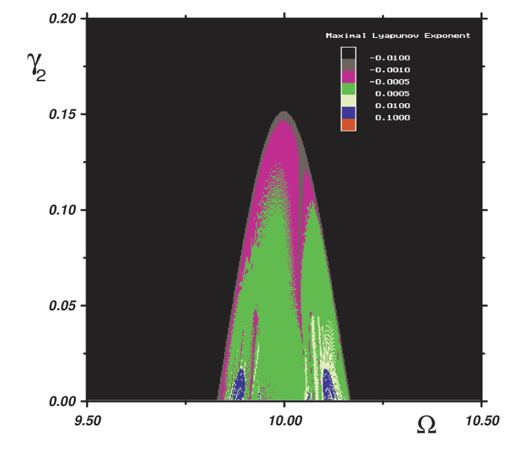
Figure 1:

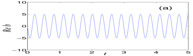
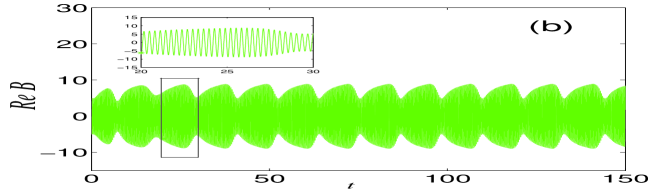
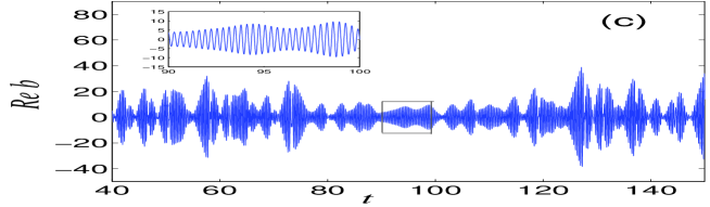
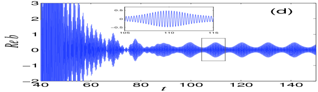
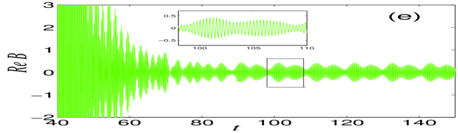
Figure 2:

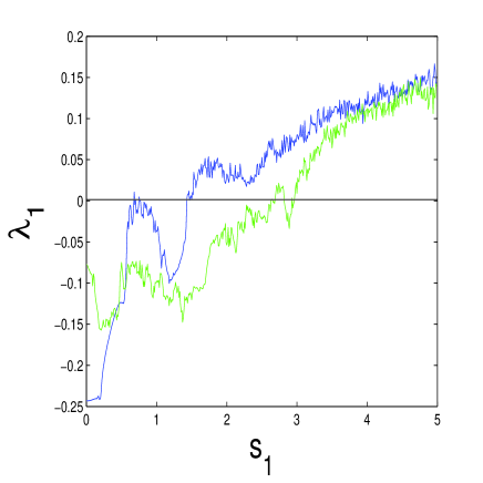
Figure 3:

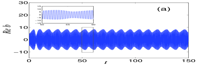
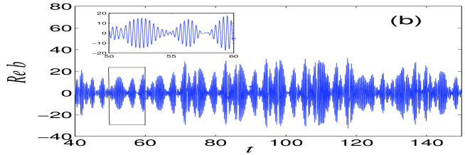
Figure 4:

References

- (1) Grygiel, K. & Szlachetka, P. [2002] ”Generation of chaotic beats”, Int. J. Bifurcation and Chaos 12, 635-644.
- (2) Cafagna, D. & Grassi, G. [2004] ”A new phenomenon on nonautonomous Chua’s circuits: generation of chaotic beats”, Int. J. Bifurcation and Chaos 14, 1773-1788.
- (3) Cafagna, D. & Grassi, G. [2004] ”Chaotic beats in a modified Chua’s circuits: dynamic behavior and circuit design”, Int. J. Bifurcation and Chaos 14, 3045-3064.
- (4) Cafagna, D. & Grassi, G. [2005] ”On the generation of chaotic beats in simple nonautonomous circuits”, Int. J. Bifurcation and Chaos 15, 2247-2256.
- (5) Cafagna, D. & Grassi, G. [2006] ”Generation of chaotic beats in a modified Chua’s circuit part I:Dynamic behaviour”, Nonlinear Dynamics 44(1-4), 91-99.
- (6) Cafagna, D. & Grassi, G. [2006] ”Generation of chaotic beats in a modified Chua’s circut part II:Circuit design”, Nonlinear Dynamics 44(1-4), 101-108.
- (7) Śliwa, I., Szlachetka, P. & Grygiel, K. [2007] ”Chaotic beats in a nonautonomous system governing second-harmonic generation of light”, Int. J. Bifurcation and Chaos in press - arXiv:nlin.CD/0609062.
- (8) Minorsky, N. [1962] Nonlinear Oscillations, Van Nostrand, Princeton.
- (9) Eberly, J. H., Narozhny, N. B., & Sanchez-Mondrogon, J. J. [1980] ”Periodic spontaneous collapse and revivals in a simple quantum model”, Phys. Rev. Lett. 44, 1323-1326.
- (10) Abdalla, M. S., Hassan, S. S., & Abdel-Aty, M. [2005] ”Entropic uncertainty in the Jaynes-Cummings model in presence of a second harmonic generation”, Opt. Commun. 244, 431-443.
- (11) Wolf, A., Swift, J.B., Swinney H.L. & Vastano, J.A. [1985] ”Determining Lyapunov exponents from a time series”, Physica D 16, 285-317.
- (12) Peŕina, J.Jr. & Peŕina, J. [2000] ”Quantum Statistics of Nonlinear Optical Couplers in Optics”, edited by E. Wolf (Elsevier Science), Vol. 41, 361-419.
- (13) Drummond, P. D., McNeil, K. J. & Walls, D. F. [1980] ”Non-equilibrium transitions in sub/second harmonic generation I. Semiclassical theory”, Opt. Acta 27(3), 321-335.
- (14) Mandel, P. & Erneux, T. [1982] ”Amplitude self-modulation of interactivity second-harmonic generation”, Opt. Acta 29, 7-21.
- (15) Gao, W. ”Study on statistical properties of chaotic laser light”, Phys. Lett. A 331, 292-297.
- (16) Rössler [1979] ”An equation for hyperchaos”, Phys. Lett. A 71, 155-157.