A New Proof of Pappus’s Theorem

Abstract.

Any stretching of Ringel’s non-Pappus pseudoline arrangement when projected into the Euclidean plane, implicitly contains a particular arrangement of nine triangles. This arrangement has a complex constraint involving the sines of its angles. These constraints cannot be satisfied by any projection of the initial arrangement. This is sufficient to prove Pappus’s theorem. The derivation of the constraint is via systems of inequalities arising from the polar coordinates of the lines. These systems are linear in $\mathbf{r}$ for any given $\boldsymbol{\theta}$, and their solubility can be analysed in terms of the signs of determinants. The evaluation of the determinants is via a normal form for sums of products of sines, giving a powerful system of trigonometric identities. The particular result is generalized to arrangements derived from three edge connected totally cyclic directed graphs, conjectured to be sufficient for a complete analysis of angle constraining arrangements of lines, and thus a full response to Ringel’s slope conjecture. These methods are generally applicable to the realizability problem for rank 3 oriented matroids.

1. Introduction

A more accurate, but less snappy, title for this paper might have been: “New Approaches to Angles and Arrangements of Lines and Pseudolines applied to Pappus’s Theorem”. This paper does contain a new proof of Pappus’s theorem, but it is fairly laborious and ugly. In particular, it is strangely asymmetric given the beauty and symmetry of the theorem being proved. The reader only wishing to be convinced of the truth of Pappus’s theorem is best advised to go elsewhere.

The hope is that the reader will find:

• A new appreciation of the complex constraints between angles in line arrangements, without regard to any distances in the arrangement.

• An awareness of the power of polar coordinates in addressing the pseudoline stretching problem.

• New techniques for decomposing pseudoline arrangements into partial arrangements by considering the orientations of only some of the triangles.

• A normal form for sums of products of sines, useful for finding complex trigonometric identities.

• A concept of twisted graph, allowing the derivation of angle constraining arrangements of lines from three edge connected graphs.

• An understanding of the potential for solving problems set in the projective plane by an analysis in the Euclidean plane.

• And, a new proof of Euclid’s porism, usually known as Pappus’s theorem.

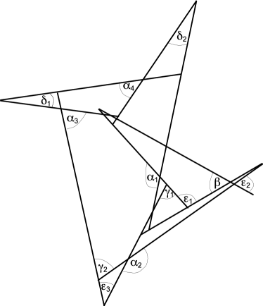
(a) The main result (E)

(b) $\mathbf{Rin}(9)$ (from [Grünbaum, 1969]) (P)

Figure 1.

1.1. Main Result

In figure 1(a), we have:

(1) $$\sin(\alpha_{1})\sin(\alpha_{2})\sin(\alpha_{3})\sin(\alpha_{4})\sin(\beta)\\ +\sin(\beta)\sin(\gamma_{1})\sin(\gamma_{2})\sin(\delta_{1})\sin(\delta_{2})\\ >\sin(\delta_{1})\sin(\delta_{2})\sin(\epsilon_{1})\sin(\epsilon_{2})\sin(\epsilon_{3})$$

This result is sufficient to show that the 9-line non-Pappus pseudoline arrangement of [Ringel, 1956], fig. 1(b), cannot be stretched, i.e. drawn with straight lines. Reversing Ringel’s non-stretchability proof from Pappus, proves Pappus from equation (1). The main result is first proved fairly directly, from Motzkin’s PhD thesis, and then as a special case of a general result which gives similar conditions to an infinite class of diagrams, for example, derivable from every cubic graph.

1.2. Angles

This paper studies the relationship between angles and the topology of line arrangements in the Euclidean plane. This presents a significant departure from previous approaches to geometry, in which either the metric plays a central role, or which abstract both from the metric and the protractor. The relationships of interest are nontrivial relationships constraining products of sines of the angles which do not involve any of the distances. Some initial examples are shown in figures 2(a), 2(b) and 2(c). For each of these the following inequality holds:

(2) $$\Pi_{i=1}^{n}\sin(\beta_{i})>\Pi_{i=1}^{n}\sin(\alpha_{i})$$

This result is derived in [Carroll, 2006], by a simple application of the sine formula to each of the exscribed larger triangles.

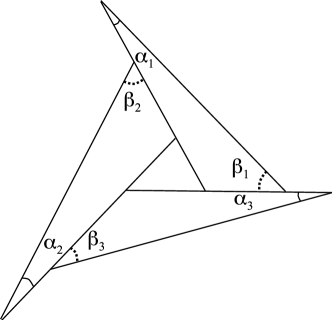
(a) n=3

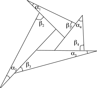
(b) n=4

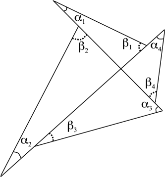
(c) n=4

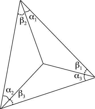
(d) Ceva

Figure 2. Circular Saws (E)

The first of these, when taken to the limit amounts to the trigonometric variation of Ceva’s theorem [Ceva, 1678] that in figure 2(d), $\Pi_{i=1}^{3}\sin(\beta_{i})=\Pi_{i=1}^{3}\sin(\alpha_{i})$.

The longterm goal of this work is to solve the pseudoline stretching problem: to provide a useable algorithm that, given a pseudoline arrangement, either provides an equivalent line arrangement or provides a proof that none exists.

2. Outline of Paper

To help the reader navigate this overly long paper, we give a detailed outline.

The next section gives an overview of the broad context of this study. Some specific conventions and notations are described in section 4; while our specific approach to polar coordinates of lines is given in section 6. The relationship between our use of polar coordinates and the chirotope of oriented matroids is given in section 6.2, which should be omitted by the reader unfamiliar with oriented matroids.

Results from the literature are given throughout the paper:

section 5:

describes pseudoline arrangements, and the stretchability problem.

section 9:

summarizes Motzkin’s version of Carver’s results concerning system of strict linear inequalities.

section 12:

discusses the oriented matroids derived from directed graphs and total orders.

The new contributions start with the statement of the main theorem in section 7.

This is used in section 8 to prove the nonstretchability of Ringel’s non-Pappus pseudoline arrangement. From this we derive Pappus’s theorem. This derivation is included principally to justify the title of this paper. The specialist reader may wish to skip it. The more general reader may find that it relates the somewhat esoteric topic of oriented matroid realizability with something more familiar. Section 8 starts with a brief look at Pappus’s own work, including, notably, two of Pappus’s own diagrams, again aimed at the more general reader.

The first proof of the main theorem is given in section 11. This tedious proof involves the computation of the signs of twenty two determinants of sub-matrices from a particular nine by ten matrix, encapsulating fig.  1(a).

The computations in that proof depend on the manipulation of sums of products of sines. Hence, section 10 explores such sums, giving a simple method of expanding them to normal form, much simplifying section 11. Unfortunately, the methods used to prove the correctness of the normal form depend on multisets and I was unable to find an appropriate treatment in the literature, so that section 10.1 gives a quick overview, extending the description from Wikipedia to permit a finite power multiset operation. Thus section 10 consists of two digressions, and should probably be omitted at first reading, except the introductory paragraphs (on the other hand, the digression is interesting in itself, and a different reader may prefer to read only that section, and omit the rest of the paper).

The most interesting new work concerns generalisations of the techniques used to prove the main theorem. These are given in sections 13, 14 and 15. The first of these introduces the notion of a twisted graph, generalizing the line arrangement studied in the main theorem. Section 15 shows that results similar to the main theorem can be derived for many twisted graphs, including all totally cyclic, simply three edge connected, directed cubic graphs. Conjectures of stronger results are made.

The final discussion, in section 16, concerns how these results may be relevant to the pseudoline stretching problem, giving (without proof), a cryptomorphic axiom system for rank 3 acyclic oriented matroids, suited for studying partial line arrangements in the Euclidean plane. We suggest that every unrealizable rank 3 oriented matroid contains a line arrangement that is a counterexample to Ringel’s slope conjecture, thus showing that the proof technique used to prove the unstretchability of the non-Pappus arrangement is general. We discuss future directions for this work.

The paper closes with a brief conclusion.

3. Context and Related Work

3.1. Euclidean Geometry

Euclidean geometry is the oldest area of mathematical study, but is nowadays seen as essentially completed and not an area for research. One of the claims of this paper is that angles have not been studied adequately independently of the metric in Euclidean geometry (unlike the metric independently of angles). As well as the angular variant of Ceva’s theorem, there is a small amount of recent work on angles independent of distance, such as the study of the angles formed by $n$-points in the plane, specifically the greatest least angle [Jaudon and Parlier, 2006] and the least greatest angle [Sendov, 1995].

The ancients accounted for linear constraints on angles, such as the angle sum of a triangle, and the angles formed by a transversal of parallel lines. However, their emphasis was on results whose primary focus is distance or area, such as Pythagoras’ theorem.

Later, the introduction of Cartesian coordinates put a further emphasis on distance, at the expense of angles. Trigonometry, of course, does give angles a central role, but rarely to the exclusion of distance.

As modern geometry developed, either both angles and distances were retained (e.g. hyperbolic geometry), or angles got abstracted away (projective geometry) , or both distances and angles vanish in the abstraction.

3.2. Pseudoline Arrangements

Pseudolines were introduced by [Levi, 1926], who along with most authors (such as [Ringel, 1956]), work in the projective plane. A seminal paper is ‘The Importance of Being Straight’ [Grünbaum, 1969]. A core problem in the study of pseudolines is stretchability: given a pseudoline arrangement is there an equivalent line arrangement.

In this paper, because of the focus on angles, we work primarily in the Euclidean plane. This preference is shared with some other authors such as [Felsner, 1997, Felsner and Weil, 1999, Sharir and Smorodinsky, 2001, Agarwal and Sharir, 2002, Shor, 1991]. The definition used by most of these is that a pseudoline is an $x$-monotone curve in the Euclidean plane; and in an arrangement of pseudolines every pair meet exactly once, at a point where they cross. This definition commits to a Cartesian coordinate system, whereas we work in polar coordinates. [Shor, 1991] works in the Euclidean plane and allows more general pseudolines (“the image of a line under a homeomorphism of the plane”) and permits ‘parallel’ pseudolines that do not meet. In contrast, we follow [Felsner and Kriegel, 1999], and define pseudolines in the projective plane, but work in the Euclidean plane.

We note that line arrangements (in the Euclidean plane) were a major focus of mathematics for over a millennium.

The pseudoline stretchability problem is known to be NP-hard [Shor, 1991]. Moreover, via the relationship to oriented matroids, it is known to be polynomial time equivalent to the existential theory of the reals, (i.e. multivariate polynomial programming) [Mnëv, 1988].

3.3. Oriented Matroids

The projective plane appears most forcefully in the correspondence between pseudolines and oriented matroids given by the topological representation theorem of [Folkman and Lawrence, 1978]. In this, the problem of pseudoline stretchability is equivalent to the problem of rank 3 oriented matroid realizability. Every rank 3 oriented matroid can be represented by a pseudoline arrangement. Realizable oriented matroids can be represented by a line arrangement. Other authors study oriented matroids via the chirotope, which, in line arrangements, corresponds naturally to determinants of homogeneous coordinates (in the projective plane). Most progress on oriented matroid realizability has been made in such terms. For example, Bokowski’s algorithm for finding biquadratic final polynomials can be applied to the oriented matroid $\mathbf{Rin}(9)$ to prove its nonrealizability. The main result of this paper is equivalent. The invaluable standard reference for oriented matroids is [Björner et al., 1999].

3.4. Ringel’s Slope Conjecture

[Ringel, 1956] conjectured that in an arrangement of lines in general position the slopes could be arbitrarily prescribed. This conjecture was disproved first by [Las Vergnas, 1986] using oriented matroid techniques over a 32 point dual construction. [Richter-Gebert and Sturmfels, 1991] improved this to give a 6 line counterexample (fig. 2(c)), still demonstrating the slope constraint using oriented matroid techniques. [Felsner and Ziegler, 2001] give a different proof of the counterexample using higher Bruhat orders. [Carroll, 2006] demonstrates the result using schoolbook geometry. The main theorem of this paper is another counter-example. The theme of the more general analysis of this paper, sections 13 to 16, is the search for all minimal counter-examples to this conjecture.

3.5. Venn Triangles

This paper builds on my earlier work which suffers from complete ignorance of the field. This was motivated by a specific pseudoline stretching problem, relating to drawing diagrams of 6-Venn triangles [Carroll, 2000c]. While I produced a pseudoline stretching program that stretched the diagrams of interest to me at that time, I could not adequately explain why it worked. This paper is a move towards an explanation. The key insight of my earlier work, that is not in the literature, is that the use of polar coordinates allow the pseudoline stretching problem to be divided into two separate phases: first determine the $\boldsymbol{\theta}$ coordinates of the lines, and second, use linear programming techniques to determine the $\mathbf{r}$ coordinates. The latter step is a solved problem, although issues are presented by the linear program being over the reals rather than the rationals; and by the extensive use of strict inequalities. Thus, my primary interest is the first problem of what are the nonlinear constraints placed on angles by line arrangements, such as those illustrated by figures 1(a) and 2.

4. Notation and Conventions

4.1. Geometry of Diagrams

Some of the diagrams, e.g. fig. 1(a), illustrate the Euclidean plane, and the choice of the line at infinity is significant. These are marked with an (E). Others, e.g. fig. 1(b), illustrate the projective plane, and no significance should be read into the particularly choice of the projection used for the illustration. These are marked with a (P). Figs. 7(a) and 7(b) on page 7(a), explicitly show the line at infinity, as an oval around the diagram.

4.2. Graphs, Directed Graphs

We use simple graphs and directed graphs, both restricted to be loop free and without parallel or antiparallel edges. Fig. 9 on page 9 shows a simple graph and a directed graph, the latter also intended to have a Euclidean reading.

4.3. Polar Coordinates

We use polar coordinates extensively. They always refer to lines rather than points. A pair of polar coordinates $(r_{i},\theta_{i})$ refer to the $i$th line, with $r_{i}$ being the perpendicular distance from the origin to the line, and $\theta_{i}$ is the angle that the perpendicular makes with the polar direction.

In diagrams, we always place the origin at the far lower edge of the plane, in an unbounded region, which is not cut by any of the lines (or their extensions), in the picture. We represent the origin either: as in figure 3(a), like:

to indicate its exact position; or, as in figure 4, like:

to indicate that the origin lies directly below the indicated position, sufficiently far to lie in an unbounded region.

This choice of positioning ensures that in the diagrams $r_{i}>0$ and $0<\theta_{i}<180$ for all lines $i$, and is formally validated in lemma 6.1.

4.4. Sines

This paper deals extensively with the relationships between the sines of different angles in line arrangements. In terms of the polar coordinates such sines are $\sin(\theta_{j}-\theta_{i})$. We abbreviate this as $S^{j}_{i}$. i.e.

(3) $$S^{j}_{i}=\sin(\theta_{j}-\theta_{i})$$

4.5. Partial and Total Orders

We use $\prec$ to represent partial orders, and $<$ to represent total orders. The distinction is particularly pertinent in sections 13 to 15.

4.6. Matrices

We make extensive use of matrices with a specific form. Each row has three non-zero entries. If the non-zero columns are $i,j,k$ then the non-zero values are either: $\sin(\theta_{k}-\theta_{j}),-\sin(\theta_{k}-\theta_{i}),\sin(\theta_{j}-\theta_{i})$ or $-\sin(\theta_{k}-\theta_{j}),\sin(\theta_{k}-\theta_{i}),-\sin(\theta_{j}-\theta_{i})$. In all cases the sines themselves are positive. For example,

(4) $$M=\left(\begin{smallmatrix}&S^{6}_{4}&&-S^{6}_{2}&&S^{4}_{2}\\ S^{3}_{2}&-S^{3}_{1}&S^{2}_{1}&&&\\ -S^{5}_{4}&&&S^{5}_{1}&-S^{4}_{1}&\\ &&-S^{6}_{5}&&S^{6}_{3}&-S^{5}_{3}\end{smallmatrix}\right)$$

abbreviates:

(5) $$M=\left(\begin{smallmatrix}0&\sin(\theta_{6}-\theta_{4})&0&-\sin(\theta_{6}-\theta_{2})&0&\sin(\theta_{4}-\theta_{2})\\ \sin(\theta_{3}-\theta_{2})&-\sin(\theta_{3}-\theta_{1})&\sin(\theta_{2}-\theta_{1})&0&0&0\\ -\sin(\theta_{5}-\theta_{4})&0&0&\sin(\theta_{5}-\theta_{1})&-\sin(\theta_{4}-\theta_{1})&0\\ 0&0&-\sin(\theta_{6}-\theta_{5})&0&\sin(\theta_{6}-\theta_{3})&-\sin(\theta_{5}-\theta_{3})\end{smallmatrix}\right)$$

For large such matrices, for convenience, we add explicit row and column labels, e.g.

(6) $$M=\begin{pmatrix}&(1)&(2)&(3)&(4)&(5)&(6)\\ (A)&&S^{6}_{4}&&-S^{6}_{2}&&S^{4}_{2}\\ (B)&S^{3}_{2}&-S^{3}_{1}&S^{2}_{1}&&&\\ (C)&-S^{5}_{4}&&&S^{5}_{1}&-S^{4}_{1}&\\ (D)&&&-S^{6}_{5}&&S^{6}_{3}&-S^{5}_{3}\end{pmatrix}$$

We represent submatrices formed by columns using the notation $M\left[2,3,6\right]$. Thus:

(7) $$M\left[2,3,6\right]=\begin{pmatrix}S^{6}_{4}&0&S^{4}_{2}\\ -S^{3}_{1}&S^{2}_{1}&0\\ 0&0&0\\ 0&-S^{6}_{5}&-S^{5}_{3}\end{pmatrix}$$

5. Pseudolines

Most authors, following Levi, work in the projective plane. [Grünbaum, 1969]:

an arrangement of pseudolines is a finite family [with at least two member] of simple closed curves in the projective plane, such that every two curves have exactly one point in common, each crossing the other at this point, while no point is common to all the curves.

A pseudoline $L$, like a projective line, is such that $\mathbb{P}^{2}\setminus L$ is connected. A family of non-coincident lines in the projective plane satisfy this definition, so that every arrangement of lines is an arrangement of pseudolines.

Two pseudoline arrangements are equivalent if there is a homeomorphism from one to the other. A pseudoline arrangement is stretchable if it is equivalent to a line arrangement.

Our use of polar coordinates commits to a Euclidean viewpoint, and not the usual one of $x$-monotone lines. Following [Felsner and Kriegel, 1999] we use Levi’s definition, but fix a line at infinity, with a homeomorphism followed by a projection, and then work in the Euclidean plane.

6. Polar Coordinates of Line Arrangements

6.1. Polar Coordinates

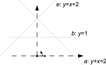
(a) A positive triangle

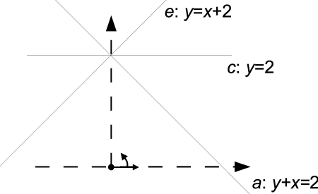
(b) Coincident lines

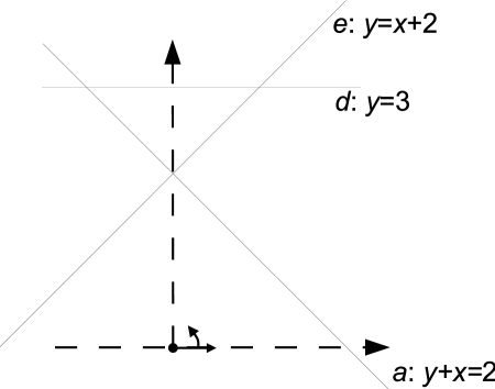
(c) A negative triangle

Figure 3. Arrangements of three lines (E)

The polar coordinates of a line are given as the coordinates of the point where a perpendicular to the origin can be drawn. In figure 3(a), for line (a) the point has cartesian coordinates $(1,1)$, or polar coodinates $(\surd{2},45)$. Similarly, line (b) is given by $(1,90)$, and line (e) by $(\surd{2},135)$.

For any three coincident lines as in fig. 3(b), if the lines have coordinates $(r_{i},\theta_{i})$, with $i$ from 1 to 3, and $\theta_{i}$ increasing, the following identity holds:

(8) $$r_{1}\sin(\theta_{3}-\theta_{2})-r_{2}\sin(\theta_{3}-\theta_{1})+r_{3}\sin(\theta_{2}-\theta_{1})=0$$

If the three lines form a positively oriented triangle, with the origin in an unbounded face with three edges, as in fig. 3(a), then this identity becomes an inequality:

(9) $$r_{1}\sin(\theta_{3}-\theta_{2})-r_{2}\sin(\theta_{3}-\theta_{1})+r_{3}\sin(\theta_{2}-\theta_{1})>0$$

If the three lines form a negatively oriented triangle, with the origin in an unbounded face with two edges, as in fig. 3(c), then the inequality is reversed in sign:

(10) $$-r_{1}\sin(\theta_{3}-\theta_{2})+r_{2}\sin(\theta_{3}-\theta_{1})-r_{3}\sin(\theta_{2}-\theta_{1})>0$$

These results can be proved directly using schoolbook geometry. [Carroll, 2000a] uses trilinear coordinates [Coxeter, 1995, Plücker, 1835].

We do not consider the case when the origin is inside a triangle, preferring to only use coordinate systems with origins towards the edge of the plane, to ensure that this does not happen. We also choose the coordinate system (particularly the location of the origin), so that $0<\theta<180$ for all angles $\theta$ of interest. In the next subsection, we derive both the above inequalities, and formalize the choice of coordinate system in terms of oriented matroid theory. This can be skipped by the uninterested reader.

6.2. Chirotopes and the Choice of Polar Origin (optional)

Given a line arrangement in the Euclidean plane, we have argued above that the polar origin can always be placed in such a way that all the lines have angles between 0 and 180. In this section, we formalise the argument in terms of the chirotope of a rank 3 acyclic oriented matroid. Given such a line arrangement, indexed by a set $X$, we can form a set $E=X\cup\{\omega\}$, and take homogenous coordinates for $E$, with $\omega$ representing the line at infinity. We label some face adjacent to $\omega$ and not between parallel lines, as the positive tope, and hence choose an acylic orientation for the matroid, along with a particular realization. We can then apply the following lemma, which shows how to compute polar coordinates with the desired property, and hence locate a polar origin.

Lemma 6.1.

For a rank 3 acyclic oriented matroid $\mathcal{M}$, with chirotope $\chi:E^{3}\rightarrow\{-1,0,1\}$ with $E=X\mathaccent 0{\cdot}\cup\{\omega\}$, with $\omega$, not being a coloop, nor parallel or antiparallel, to any other element, and with distinct positive cocircuits $A$, $B$ neither containing $\omega$, such that for all $a\in A\setminus B$ and $b\in B\setminus A$, $\chi(\omega,a,b)=1$, and with a realization given by $\mathbf{v}_{e}=\left(\begin{smallmatrix}x_{e}\\ y_{e}\\ z_{e}\end{smallmatrix}\right)\in\mathbb{R}^{3}$, for each $e\in E$, then the $\mathbf{v}_{e}$ can be chosen such that:

1. $\mathbf{v}_{\omega}=\left(\begin{smallmatrix}0\\ 0\\ 1\end{smallmatrix}\right)$

2. $x_{a}^{2}+y_{a}^{2}=1$ for all $a\in X$

3. There are $\theta_{a}\in[0,360)$, such that $x_{a}=-cos(\theta_{a})$, $y_{a}=-sin(\theta_{a})$ for each $a\in X$.

4. There are $\theta_{a}\in[0,180)$, such that $x_{a}=-cos(\theta_{a})$, $y_{a}=-sin(\theta_{a})$ for each $a\in X$.

5. There are $\theta_{a}\in(0,180)$, such that $x_{a}=-cos(\theta_{a})$, $y_{a}=-sin(\theta_{a})$ for each $a\in X$.

6. $z_{a}>0$ for each $a\in X$

7. There are $(r_{a},\theta_{a})_{a\in X}\in\mathbb{R}^{+}\times(0,180)$ such that equations (8, 9, 10) hold, depending on whether the corresponding value of $\chi$ is 0, 1 or -1, respectively.

8. $(r_{a},\theta_{a})_{a\in X}$ are polar coordinates for the realization, given an appropriate origin.

Proof.

If this is not true, then for one of the claims we can find a realization $\mathbf{v}_{e}$ that satisfies the previous claims, and there is no realization that satisfies both the previous claims and the new claim. We will show this leads to a contradiction, by constructing a realization $\mathbf{v^{\prime}}_{e}$.

At each stage, we do one of:

• take $\mathbf{v^{\prime}}_{e}=\mathbf{v}_{e}$ for all $e\in E$.

• Give a matrix $P$ with positive determinant, and take $\mathbf{v^{\prime}}_{e}=P\mathbf{v}_{e}$ for all $e\in E$.

• Give $\lambda_{e}>0$ for each $e\in E$, and take $\mathbf{v^{\prime}}_{e}=\lambda_{e}\mathbf{v}_{e}$

Each of these steps leaves the signs of the subdeterminants unchanged, so that $\mathbf{v^{\prime}}_{e}$ is a realization of $\mathcal{M}$.

We use a total order $\leq$ over $E\setminus\{\omega\}$, defined by:

(11) $$x\leq y\text{ if and only if }\chi(\omega,x,y)\geq 0$$

This is transitive and reflexive since $\chi(\omega,x,y)$ is the chirotope of the acyclic rank 2 oriented matroid, $\mathcal{M}\setminus\{\omega\}$.

1. From the two cocircuits we can find $a,b\in X$, with $a<b$. Take $P=\begin{pmatrix}\mathbf{v}_{a}&\mathbf{v}_{b}&\mathbf{v}_{\omega}\end{pmatrix}^{-1}$.

2. Take

   (12) $$\lambda_{e}=\begin{cases}1_{e}&e=\omega\\ (x_{a}^{2}+y_{a}^{2})^{-1/2}&\text{otherwise}\end{cases}$$

3. Unchanged.

4. Take $a\in A\setminus B$, then for all $b\in X$, $a\leq b$. Take

   (13) $$P=\begin{pmatrix}cos(\theta_{a})&sin(\theta_{a})&0\\ -sin(\theta_{a})&cos(\theta_{a})&0\\ 0&0&1\end{pmatrix}$$

   Since $\chi(\omega,a,b)=1$, for $b\in X$, we have $\sin(\theta^{\prime}_{b}-\theta^{\prime}_{a})>0$, and $\theta^{\prime}_{a}=0$, this ensures that $\theta^{\prime}_{b}<180$.

5. For some sufficiently small $\epsilon$, take

   (14) $$P=\begin{pmatrix}cos(\epsilon)&-sin(\epsilon)&0\\ sin(\epsilon)&cos(\epsilon)&0\\ 0&0&1\end{pmatrix}$$

6. For every $a\in X$, $y_{a}=-sin(\theta_{a})<0$. So we can choose some $\mu$ sufficiently large such that, for all $a\in X$, $\mu>z_{a}/y_{a}$ so that $z_{a}-\mu y_{a}>0$. Take

   (15) $$P=\begin{pmatrix}1&0&0\\ 0&1&-\mu\\ 0&0&1\end{pmatrix}$$

7. Take $r_{a}=z_{a}$.

8. Nothing to prove.

∎

While the conditions on this theorem seem a bit restrictive, they do not hinder our purposes, for a Euclidean line arrangement, the process of adding $\omega$ as the line at infinity, ensures the constraints on $\omega$ hold; and we can then find an acyclic orientation with an appropriate positive tope, such that $X$ is a positive vector, and satisfying the conditions on the positive cocircuits $A$ and $B$. The only resulting constraint is that we cannot place the origin between parallel lines, which is obvious.

7. Statement of Main Theorem

Using the notion of positively and negatively oriented triangles, we can now formally state the main theorem, which is illustrated in figure 4. The labels correspond to the figures in the next section: the numbers labelling the lines, the letters labelling shaded regions.

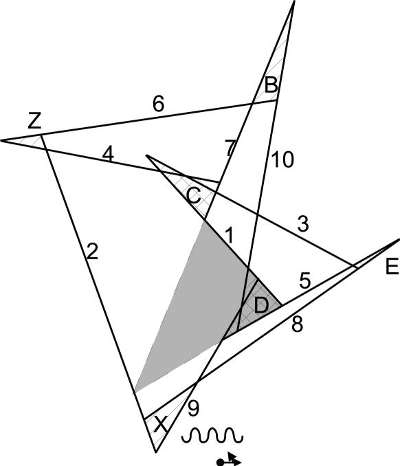
Figure 4. Illustrating the main theorem (E)

Theorem 7.1.

In any arrangement of 10 lines with polar coordinates $\{(r_{i},\theta_{i}):i=1,\ldots 10\}$, in which the triangles $(2,4,6)$, $(1,5,9)$, $(1,5,10)$, $(1,5,7)$ are positively oriented, and the triangles $(1,3,7)$, $(1,4,7)$, $(3,5,8)$, $(2,8,9)$, $(6,7,10)$, are negatively oriented, we have:

(16) $$\sin(\theta_{9}-\theta_{8})\sin(\theta_{10}-\theta_{1})\sin(\theta_{4}-\theta_{2})\sin(\theta_{5}-\theta_{3})\sin(\theta_{7}-\theta_{6})\\ +\sin(\theta_{6}-\theta_{4})\sin(\theta_{9}-\theta_{1})\sin(\theta_{10}-\theta_{7})\sin(\theta_{5}-\theta_{3})\sin(\theta_{8}-\theta_{2})\\ -\sin(\theta_{6}-\theta_{4})\sin(\theta_{8}-\theta_{3})\sin(\theta_{10}-\theta_{7})\sin(\theta_{9}-\theta_{2})\sin(\theta_{5}-\theta_{1})>0$$

where, for each of the nine specified triangles, $(i,j,k)$, we have $0<\theta_{i}<\theta_{j}<\theta_{k}<180$.

Note, that except as specified, we do not require $\theta_{i}<\theta_{j}$ when $i<j$. For example, $\theta_{2}$ may be less than or equal to $\theta_{1}$, as in fig. 4.

Two proofs are given, the first in section 11, is a direct computation specific to this figure. This approach is then generalised in section 15, and this specific result is derived on page 15.2 from a more general theorem.

From the discussion in section 6, we see that such a figure can be drawn if, and only if, the following system of inequalities is soluble:

(17) $$\left(\begin{smallmatrix}&&-S^{8}_{5}&&S^{8}_{3}&&&-S^{5}_{3}&&\\ &-S^{9}_{8}&&&&&&S^{9}_{2}&-S^{8}_{2}&\\ &S^{6}_{4}&&-S^{6}_{2}&&S^{4}_{2}&&&&\\ &&&&&-S^{10}_{7}&S^{10}_{6}&&&-S^{7}_{6}\\ -S^{7}_{3}&&S^{7}_{1}&&&&-S^{3}_{1}&&&\\ -S^{7}_{4}&&&S^{7}_{1}&&&-S^{4}_{1}&&&\\ S^{9}_{5}&&&&-S^{9}_{1}&&&&S^{5}_{1}&\\ S^{10}_{5}&&&&-S^{10}_{1}&&&&&S^{5}_{1}\\ S^{7}_{5}&&&&-S^{7}_{1}&&S^{5}_{1}&&&\end{smallmatrix}\right)\boldsymbol{r}>\boldsymbol{0}$$

The resulting $\boldsymbol{r}$ gives the $r_{i}$ coordinates of a drawing of the figure.

For fixed $\boldsymbol{\theta}$, this is a linear program in $\boldsymbol{r}$. The solubility of linear programs is a well-understood problem, and we spend section 9 reviewing some results from Motzkin’s PhD thesis.

8. Pappus’s Theorem

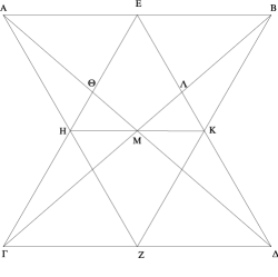
(a) Pappus folio 161v (E)

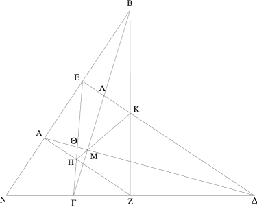
(b) Pappus folio 162 & Jones’s fig. 139 (E)

Figure 5. Figures from [Pappus, c340], [Pappus and Jones, 1986a]

In [Pappus, c340], Pappus of Alexandria proves numerous lemmas concerning Euclid’s Porisms [Euclid, c300BC]. The combination of several, have become known as Pappus’s Theorem. A porism may have been a general statement linked to more specific examples, in which case, Pappus’s contribution of enumerating the cases and proving each, would indeed merit the general attribution of the theorem to him. Concerning the origin of the general statement, even Pappus’s attribution to Euclid may be insufficiently ancient: at least some commentators view Euclid as a master compiler, rather than a deep original thinker, which would suggest that Euclid’s lost Porisms, would in turn credit yet older work.

Pappus’s statement of the lemmas, follows the convention that the order of points on a line, and the definition of points that are the intersections of lines is often left to the reader’s consulting of the drawing, see [Pappus and Jones, 1986a]. The two drawings for these lemmas are taken from the earliest extant, tenth century, copy of [Pappus, c340], held in the Vatican library. We’ve copied Jones’ copies [Pappus and Jones, 1986b], including his correction to fig. 5(b) of an error in the Vaticanus, detailed on his page 624. Jones notes in [Pappus and Jones, 1986a] that Pappus’s diagrams, following the conventions of the time, have a pronounced preference for symmetry and regularization. In particular, line $HMK$ need not be horizontal in figure 5(a), and none of the lines need be perpendicular in figure 5(b).

Two of the relevant lemmas of Pappus are:

Lemma 8.1.

Figure 5(a). [Pappus, c340] (folio 161v in Vatican copy) Now that these things have been proved, let it be required to prove that, if $AB$ and $\Gamma\Delta$ are parallel, and some straight lines $A\Delta$, $AZ$, $B\Gamma$, $BZ$ intersect them, and $E\Delta$ and $E\Gamma$ are joined, it results that the (line) through $H$, $M$ and $K$ is straight.

Lemma 8.2.

Figure 5(b). [Pappus, c340] (folios 161v, 162, in Vatican copy) But now let $AB$ and $\Gamma\Delta$ not be parallel, but let them intersect at $N$. That again the (line) through $H$, $M$ and $K$ is straight.

Combined, with the other cases considered by Pappus, these form a single theorem, which we state in the projective plane, with more modern sensibilities, illustrated with the less regular figure 6(a), which is labelled with Latin rather than Greek letters.

(a) Pappus’s Theorem

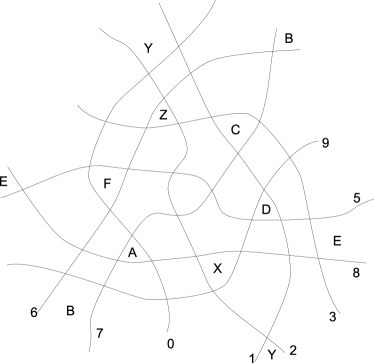
(b) $\mathbf{Rin}(9)$ labelled

Figure 6. Pappus and non-Pappus (P)

Theorem 8.3.

In the projective plane, if A, B, and C are three points on one line, D, E, and F are three points on another line, and AE meets BD at X, AF meets CD at Y, and BF meets CE at Z , then the three points X, Y, and Z are collinear.

8.1. Ringel’s non-Pappus Arrangement

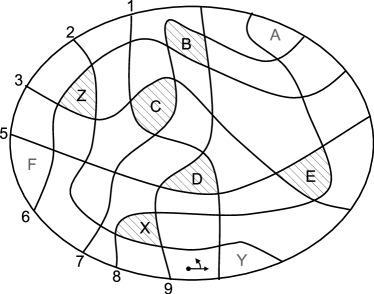
(a) Projecting on 0

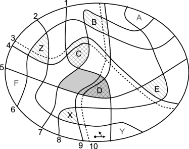
(b) Adding $4\parallel 3$ and $10\parallel 9$

Figure 7. Stretching $\mathbf{Rin}(9)$ in the Euclidean plane

We start by proving that $\mathbf{Rin}(9)$ is unstretchable. Our proof below is new, and, I assert, interesting! The result is well-known: [Ringel, 1956] works from Pappus, and [Björner et al., 1999] provide a final polynomial (see our equation (96) on page 96) which proves this independently of Pappus.

The remainder of the proof of Pappus, is an unsurprising reversal of Ringel’s argument.

The two proofs in this section proceed by contradiction, and are heavily illustrated. Thus, we need to draw impossible illustrations. We do this by representing hypothesised lines by actual pseudolines, hypothesised to be straight. The proofs argue to some extent ‘from the picture’. These arguments fundamentally concern the relative ordering of various points, on various lines, where the illustrations serve to capture the relative orderings, and what is known about them. For such arguments, pseudoline arrangements suffice. Indeed, in this paper, as in most of the literature, Ringel’s non-Pappus arrangement is not even defined, except by a picture. Formally, we could give a chirotope of the oriented matroid, this would then relate to equation (8) and its variations, to describe the significant relationships between sets of three lines in each picture; however, we choose not to.

The labels in figures 6(a), 7, 8(a), 8(c) and 8(e), are all consistent with each other and figs 4 and 9. For example, the triangle labelled $E$ in fig. 4 corresponds to the point labelled $E$ in figs 6(a) and 8(c) and to the vertex labelled $E$ in fig. 9.

We use the following technical lemma:

Proposition 8.4.

For any real $\theta_{a},\theta_{b},\theta_{c}$ and $\theta_{d}$:

(18) $$\sin(\theta_{c}-\theta_{a})\sin(\theta_{d}-\theta_{b})=\sin(\theta_{b}-\theta_{a})\sin(\theta_{d}-\theta_{c})+\sin(\theta_{d}-\theta_{a})\sin(\theta_{c}-\theta_{b})$$

The proof is an exercise. We will only use this with $a<b<c<d$. This allows us to expand any sum of products of sines of angles in a line arrangement into a sum of products of non-overlapping angles (i.e. every pair of pairs is disjoint or nested). Section 10 is an in-depth study of consequences of this lemma.

In the following proof, we project one of the pseudolines of $\mathbf{Rin}(9)$ to the line at infinity, so that we have a Euclidean arrangement of eight pseudolines. This technique was suggested by [Lawrence, 1983], and drawn explicitly in figure 1 in [Gioan and Las Vergnas, 2004].

Lemma 8.5.

$\mathbf{Rin}(9)$ is unstretchable.

Proof.

Refer to fig. 6(b). Take the line 0, and project the figure onto the Euclidean plane, with line 0 as the line at infinity, see fig. 7(a). If $\mathbf{Rin}(9)$ is stretchable, then we can take 6(b) as a line arrangement. The projection is then also a line arrangement. We choose a coordinate system with polar origin as indicated in the face bounded by lines 0, 1, 2 and 9. We draw a line 10 parallel to line 9, and a line 4 parallel to line 3; in the simplest version, we draw these two parallel lines directly on top of lines 9 and 3 respectively. In the illustration 7(b), we have drawn them slightly to one side, but leaving the relationship with the other lines, and the origin, unchanged. Fig. 7(b), being a line diagram (despite appearances), then satisfies the conditions for theorem 7.1. Moreover:

• $\theta_{3}=\theta_{4}$

• $\theta_{9}=\theta_{10}$

• and $\theta_{i}<\theta_{j}$ and $\sin(\theta_{j}-\theta_{i})>0$ for all $i<j$

Therefore, we have:

(19) $$S^{9}_{8}S^{9}_{1}S^{3}_{2}S^{5}_{3}S^{7}_{6}+S^{6}_{3}S^{9}_{1}S^{9}_{7}S^{5}_{3}S^{8}_{2}-S^{6}_{3}\mathbf{{\boldsymbol{S}}^{8}_{3}}S^{9}_{7}\mathbf{{\boldsymbol{S}}^{9}_{2}}\mathbf{{\boldsymbol{S}}^{5}_{1}}>0$$

from theorem 7.1.

We apply proposition 8.4 twice to part of the last term. We use bold terms to indicate the parts to be expanded.

(20) $$S^{8}_{3}\mathbf{{\boldsymbol{S}}^{5}_{1}}\mathbf{{\boldsymbol{S}}^{9}_{2}}$$

(21) $$= \mathbf{{\boldsymbol{S}}^{8}_{3}}S^{9}_{1}\mathbf{{\boldsymbol{S}}^{5}_{2}}+S^{8}_{3}S^{2}_{1}S^{9}_{5}$$

(22) $$= S^{9}_{1}S^{8}_{2}S^{5}_{3}+S^{9}_{1}S^{3}_{2}S^{8}_{5}+S^{8}_{3}S^{2}_{1}S^{9}_{5}$$

Substituting this into (19), and simplifying gives:

(23) $$S^{9}_{8}S^{9}_{1}S^{3}_{2}S^{5}_{3}S^{7}_{6}-\mathbf{{\boldsymbol{S}}^{6}_{3}}\mathbf{{\boldsymbol{S}}^{9}_{7}}S^{9}_{1}S^{3}_{2}\mathbf{{\boldsymbol{S}}^{8}_{5}}-S^{6}_{3}S^{9}_{7}S^{8}_{3}S^{2}_{1}S^{9}_{5}>0$$

Again, we expand one part of the middle term:

(24) $$S^{6}_{3}\mathbf{{\boldsymbol{S}}^{9}_{7}}\mathbf{{\boldsymbol{S}}^{8}_{5}}$$

(25) $$= \mathbf{{\boldsymbol{S}}^{6}_{3}}\mathbf{{\boldsymbol{S}}^{7}_{5}}S^{9}_{8}+S^{6}_{3}S^{9}_{5}S^{8}_{7}$$

(26) $$= S^{5}_{3}S^{7}_{6}S^{9}_{8}+S^{7}_{3}S^{6}_{5}S^{9}_{8}+S^{6}_{3}S^{9}_{5}S^{8}_{7}$$

Substituting into equation (23) gives

(27) $$-S^{9}_{1}S^{3}_{2}S^{7}_{3}S^{6}_{5}S^{9}_{8}-S^{9}_{1}S^{3}_{2}S^{6}_{3}S^{9}_{5}S^{8}_{7}-S^{6}_{3}S^{9}_{7}S^{8}_{3}S^{2}_{1}S^{9}_{5}>0$$

which is a contradiction, proving the lemma. ∎

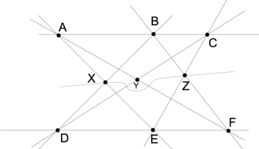
(a) A counterexample (E)

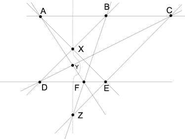
(b) A 2nd counterexample (E)

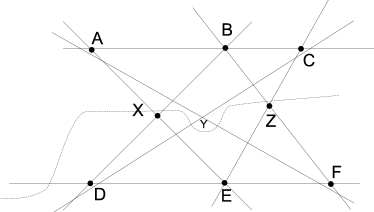
(c) Perturbing lines AF,CD,XY (E)

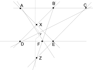
(d) Perturbing lines AF,CD,XY (E)

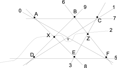
(e) Perturbing lines AC,DF (P,E)

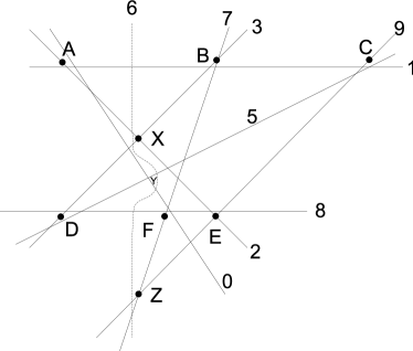
(f) Perturbing lines AC,DF (P,E)

Figure 8. Illustrating the proof

8.2. Relationship with Pappus

Proof of Pappus’s theorem 8.3.

Let N be the point of intersection of the two lines.

If N, A, B, C, D, E and F are not all distinct, then the theorem is trivial.

Take a counterexample to the theorem.

By relabelling we can assume that A and C are both adjacent to N on one line, and that D is adjacent to N on the other. Since A, B, D, E are in general position, we can project them to the corners of a square, fig. 8(a). Since C is adjacent to the point of intersection N, that lies at infinity, C is mapped to a point to the right of B as illustrated. Since D is adjacent to N, either F lies to the right of E as in fig. 8(a), or between D and E, as in fig. 8(b). In the first case, X and Z are distinct because neither can be E and X lies on AE and Z lies on CE. The line XZ is either parallel to DE, or not. If not, then it either intersects DE to the right of E or to the left. If it intersects to the right, we can relabel the projective points by swapping A and C, and D and F, and hence X and Z. So, in the first case, without loss of generality, we have XZ intersecting DE as illustrated, or XZ is parallel to DE.

By hypothesis Y does not lie on the line XZ. Without loss of generality we can assume that Y lies on the same side of XZ as A. Since, if not, in the first of the two cases, we can relabel the projective points swapping A and D, B and E, C and F, leaving X, Y and Z unchanged, but the newly labelled A lies in the same half plane of XZ as Y. In the second, E is adjacent to N, and we can relabel the projective points, swapping A and D, B and F and C and E, so that the points X and Y are swapped too.

Given either of these two diagrams, we can draw the corresponding diagram fig. 8(c) or 8(d) by: selecting a point P within the triangle XYZ and drawing new lines parallel and close to XY, XZ and YZ, strictly between the original line and P, while maintaining the incidence properties of the original line, with the other lines in the diagram, except at the points that lie on it. In the first case, if XY is parallel to DE we can twist the new line through a small angle, maintaining all the incidence properties, except that it intersects DE to the left of E, thus arriving at fig. 8(c).

We then draw lines parallel but close to lines AC and DE. To draw fig. 8(e) from 8(c), we add new lines below the old lines, but close enough not to flip any triangles. To draw fig. 8(f) from 8(d), we add new lines below AC and above DE.

We map the resulting line arrangement back into the projective plane.

So, to summarize, given an arrangement of nine lines in the projective plane, a counterexample to Pappus’s theorem, we can project it onto either fig. 8(a) or 8(b), considered as recording the relative incidence properties of the lines. By a sequence of operations, we can construct a different arrangement of nine lines, in the projective plane, either fig. 8(e) or 8(f), again recording the arrangement of the lines. However, the numbering of the lines in these last two figures, corresponds to the numbering in fig. 6(b), with the same incidence properties, e.g. line 0 crosses lines 1, 2, 3, 5, 6, 7, 8, 9 in order; and line 8 crosses lines 1, 9, 2, 0, 7, 6, 5 and 3 in order; these statements are true of all three diagrams. Hence they represent the same pseudoline arrangement. Thus we have constructed a stretched version of $\mathbf{Rin}(9)$, which is not possible: so Pappus is proved. ∎

9. Linear Programming

In section 7, we saw that the main theorem amounts to a question of linear programming.

This section reviews, without proof, results from [Motzkin, 1933], his seminal PhD thesis on systems of linear inequalities. These results are all expressed in terms of vertical simplexes, and with a system of $n$ unknowns and $m$ inequalities being expressed by an $m$-by-$n$ matrix $M$, multiplying a column vector of size $n$. Actually, we only care about such systems where the $n$ unknowns are the $r_{i}$ polar coordinates, and each row of the matrix $M$, has three non-zero elements, the $i$-th being $\pm\sin(\theta_{k}-\theta_{j})$, the $j$-th being $\mp\sin(\theta_{k}-\theta_{i})$ and the $k$-th being $\pm\sin(\theta_{j}-\theta_{i})$, for some $i$, $j$ and $k$.

Definition 9.1.

A matrix $M$ with $r+1$ rows and $r$ columns is a simplex if, up to multiplication by a constant, there is precisely one positive linear dependency between the rows.

Theorem 9.2.

A matrix $M$ with $r+1$ rows and $r$ columns is a simplex if and only if its $r+1$ $r$-by-$r$ subdeterminants alternate in sign.

Theorem 9.3.

Given an $m$-by-$n$ matrix $M$, the system $Mx>0$ is a minimal insoluble system if and only if there is some $m$-by-$m-1$ submatrix $S$ of $M$ such that:

• $S$ is a simplex.

• for all columns $c$ of $M$, the $m$-by-$m$ matrix $Sc$ has determinant zero.

The spirit of these results is anticipated by [Carver, 1922]; Motzkin’s statements clarify that it is sufficient to examine determinants of submatrices, which Carver mentions in passing.

Carver’s key theorem is:

Theorem 9.4.

A necessary and sufficient condition that a given system $S$ be inconsistent is that there exist a set of $m+1$ constants $k_{1},k_{2},\cdots k_{m+1}$, such that

(28) $$\sum_{i=1}^{m}k_{i}L_{i}(x)+k_{m+1}\equiv 0,$$

at least one of the $k$’s being positive, and none of them being negative.

In the terms of this paper, $k_{m+1}$ is always $0$, since our inequalities always compare with $0$. Thus, we can rearticulate this as:

Theorem 9.5.

Given an $m$-by-$n$ matrix $M$, the system $Mx>0$ is insoluble if and only if there is a non-negative, non-zero linear dependency between the rows of $M$.

10. A Normal Form for Products of Sines

In the previous section we saw that the solubility issues for the linear program introduced in section 7 are to be addressed by looking at determinants. The matrix in question has non-zero entries of the from $\sin(\theta_{j}-\theta_{i})$. Hence, we are going to consider sums of products of many such terms. We have already seen one fairly laborious application of the identity (18) to equation (19) to derive (27). The reader may fear that this process will be repeated.

Fear not!

We will show that repeated application of (18), with $a<b<c<d$ until it can no longer be applied, leads to a normal form. Despite the many choices faced while making such a derivation, the process terminates, and always at the same answer. Then, with the remainder of the paper, whenever we need to show a trigonometric identity, like that used in the proof of lemma 8.5, we will simply say, by normalization. The suspicious reader, will need, like the author, to write a simple computer program to perform the computation.

Theorem 10.1.

Given a formal expression being a sum of products of sines of differences between unknown angles, repeated expansion using equation (18) with $a<b<c<d$, always terminates at a uniquely determined normal form.

Apart from this result, this fairly long section is unused elsewhere in the paper. It is suggested that on first reading, you skip to page 11.

10.1. Multisets

We wish to represent an expression such as $\sin(\theta_{4}-\theta_{2})\sin(\theta_{3}-\theta_{1})$ as a set of pairs $\{\{2,4\},\{1,3\}\}$. However, if we use a set then the different expressions $\sin(\theta_{3}-\theta_{1})\sin(\theta_{3}-\theta_{1})$ and $\sin(\theta_{3}-\theta_{1})$ would be represented as the same set $\{\{1,3\}\}$. Therefore we will work with multisets. Unfortunately, I have failed to find an appropriate paper introducing multisets, so, in this subsection, I will give a quick introduction based on the Web page at Wikipedia

We will use the set

(29) $$\mathbb{N}^{+}=\mathbb{N}\cup\{\infty\}$$

for counting. Formally, by $\infty$ we mean $\aleph_{0}$, and the arithmetic we are using is cardinal arithmetic so that, for example:

(30) $$2-3 =0$$

(31) $$\infty+1 =1+\infty=\infty$$

(32) $$5 <\infty$$

We will also have the convention that

(33) $$\infty-\infty=0$$

Given a fixed set $X$, then a multiset $A$ is formally defined by an indicator function $\boldsymbol{1}_{A}:X\rightarrow\mathbb{N}^{+}$, which gives the multiplicities of the elements of $X$. We define the usual set operators, $\in,\cap,\cup,\setminus,\subset,|\cdot|$ over multisets. We also define three multiset specific operators $\uplus,\uparrow,\downarrow$.

(34) $$x\in A \>\>\textrm{when }\boldsymbol{1}_{A}(x)\geq 1$$

(35) $$\boldsymbol{1}_{A\cap B}(x) =\min\{\boldsymbol{1}_{A}(x),\boldsymbol{1}_{B}(x)\}$$

(36) $$\boldsymbol{1}_{A\cup B}(x) =\max\{\boldsymbol{1}_{A}(x),\boldsymbol{1}_{B}(x)\}$$

(37) $$\boldsymbol{1}_{A\setminus B} =\boldsymbol{1}_{A}-\boldsymbol{1}_{B}$$

(38) $$\boldsymbol{1}_{A\uplus B} =\boldsymbol{1}_{A}+\boldsymbol{1}_{B}$$

(39) $$A\subset B \>\>\textrm{when for all }x\in X,\;\boldsymbol{1}_{A}(x)\leq\boldsymbol{1}_{B}(x)$$

(40) $$|A| =\Sigma_{x\in X}\boldsymbol{1}_{A}(x)$$

(41) $$\boldsymbol{1}_{\downarrow A}(x) =\begin{cases}0&\textrm{when }\boldsymbol{1}_{A}(x)=0\\ 1&\textrm{otherwise}\end{cases}$$

(42) $$\boldsymbol{1}_{\uparrow A}(x) =\begin{cases}0&\textrm{when }\boldsymbol{1}_{A}(x)=0\\ \infty&\textrm{otherwise}\end{cases}$$

The sum and product operators, $\sum$, $\prod$, are defined in terms of the standard ones, using multiplicity, i.e.

(43) $$\sum_{a\in A}f(a) =\sum_{x\in X}\boldsymbol{1}_{A}(x)f(x)$$

(44) $$\prod_{a\in A}f(a) =\prod_{x\in X}f(x)^{\boldsymbol{1}_{A}(x)}$$

We see in these two expressions that the expression $a\in A$ is in some circumstances understood as itself having a multiplicity. This is particular significant in definitions of multisets in terms of other multisets, e.g.

(45) $$A =\{2,3,3,4,4,4\}$$

(46) $$B =\{a+3:a\in A\}$$

(47) $$B =\{5,6,6,7,7,7\}$$

so that the multiplicities in $A$ carry across to the multiplicities in $B$. A second example:

(48) $$A =\{2,3,3,4,4,4\}$$

(49) $$C =\{a\mod 2:a\in A\}$$

(50) $$C =\{0,0,0,0,1,1\}$$

Formally, given a multiset $A$, a predicate $P(x)$ assigning truth values to each $x\in A$ and a partial function $f:X\rightharpoonup X$ defined on all $x\in A$ with $P(x)$, we can construct the multiset $\{f(x):x\in A,P(x)\}$, with indicator function defined:

(51) $$\boldsymbol{1}_{\{f(x):x\in A,P(x)\}}(y)=\sum_{\{x\in X:\boldsymbol{1}_{A}(x)>0,P(x),y=f(x)\}}\boldsymbol{1}_{A}(x)$$

where the sum is over a set (not a multiset). If more than one occurrence of the multiset membership operator occurs in such a set definition then the second is introduced with words (like ‘such that’) indicating that it is to be read as a true/false predicate, ignoring multiplicities.

In contrast the multiset subset operator is simply a predicate, with a true or false value.

The most complex multiset operator we use is $\mathfrak{p}$ for finite powermultisets. The finite powermultiset $\mathfrak{p}A$ of a multiset $A$ contains precisely each of the finite multisets that are subsets of $A$, and each has an infinite multiplicity in $\mathfrak{p}A$:

(52) $$\mathfrak{p}A=\uparrow\{B\in X:B\subset A,|B|<\infty\}$$

Notice that this differs from the normal set definition of powerset. We will make $X$ large enough so that $B\in X$ is not restrictive .

In that definition we see that any subset of $X$ can be considered as a multiset, whose indicator function takes values in $\{0,1\}$. Likewise, any multiset whose indicator function only takes values $0$ or $1$, can be considered as a set. In particular, for any multiset $A$, $\downarrow A$ can be considered a set.

A final multiset operator is $\biguplus$, which additively combines all members of a multiset of multisets. This can be defined by:

(53) $$\boldsymbol{1}_{\biguplus A}=\sum_{a\in A}\boldsymbol{1}_{a}$$

The base set $X$ can usually be chosen large enough to contain everything of interest for a particular discussion, and hence can be ignored. Formally, for this section we will take $X$ as the smallest set containing both $\mathbb{N}$ and $\mathfrak{p}\uparrow X$. i.e. for any $x\notin X$, $\mathfrak{p}\uparrow X$ when defined over a ground of $X\cup\{x\}$ has the same elements as when defined over $X$.

Thus $X$ contains many multisets. Since $\mathfrak{p}$ introduces only finite multisets, this is adequately limited to avoid paradox, and could, with just a little bit more effort, be fully formalized within ZF. We make no further reference to $X$.

10.2. On Pairs of Integers

The set $\mathbb{N}^{(2)}$ is the set of all pairs of natural numbers. If $\{a,b\}\in\mathbb{N}^{(2)}$ then $a\neq b$.

We use a function $\tau$ to map members of $\mathbb{N}^{(2)}$ to formal expressions over a vector $\boldsymbol{\theta}$, corresponding to the sine function. i.e.

(54) $$\tau(\{a,b\})=\begin{cases}\sin(\theta_{b}-\theta_{a})&a<b\\ \sin(\theta_{a}-\theta_{b})&b<a\end{cases}$$

Technically, the range of $\tau$ is a free algebra. Given values for $\boldsymbol{\theta}\in\mathbb{R}^{\mathbb{N}}$, we can evaluate $\tau(\alpha)$, by substituting in the values for $\boldsymbol{\theta}$. We write $\tau(\alpha)(\boldsymbol{\theta})$ for this value.

The expressions of interest are those such as in equation (16). We will separate out the positive and negative terms, so that we have two expressions, each being the sum of products of sines of differences of pairs of angles.

To express products of sines, we will use finite submultisets of $\uparrow\mathbb{N}^{(2)}$, i.e. any member of $P$

(55) $$P=\mathfrak{p}\uparrow\mathbb{N}^{(2)}$$

We extend the definition of $\tau$ for $p\in P$, with

(56) $$\tau(p)=\prod_{x\in p}\tau(x)$$

For example:

(57) $$\tau(\{\{2,4\},\{2,4\},\{1,3\}\})=\sin(\theta_{4}-\theta_{2})\sin(\theta_{4}-\theta_{2})\sin(\theta_{3}-\theta_{1})$$

To express sums of products of sines, we use finite submultisets of $P$, i.e: any member of $S$

(58) $$S=\mathfrak{p}P$$

We similarly extend $\tau$ to $S$, to give the following definition of $\tau$ on $\mathbb{N}^{2}\cup P\cup S$:

(59) $$\tau(x)=\begin{cases}\sin(\theta_{b}-\theta_{a})&x=\{a,b\}\in\mathbb{N}^{(2)},a<b\\ \prod_{y\in x}\tau(y)&\textrm{when }x\in P\\ \sum_{y\in x}\tau(y)&\textrm{when }x\in S\end{cases}$$

We then define an equivalence relationship over $S$ by:

(60) $$\alpha\equiv\beta\textrm{ if and only if }\tau(\alpha)(\boldsymbol{\theta})=\tau(\beta)(\boldsymbol{\theta})\textrm{ for all }\boldsymbol{\theta}\in\mathbb{R}^{\mathbb{N}}$$

Trigonometric identities, such as in equation (106), can then be verified by gathering together the positive and negative terms, to give two members of $S$ and using the combinatoric methods of this section, to show that they are equivalent.

We are interested in the applicability of formula (18) to members of $P$ and $S$. We say

Definition 10.2.

A pair of pairs $\{x,y\}\in P$ is expandable, if there are $a,b,c,d\in\mathbb{N}$, with

(61) $$a <b<c<d$$

(62) $$x =\{a,c\}$$

(63) $$y =\{b,d\}$$

We also define the multiset $B\subset S$ (resp. $B_{0}\subset P$) of atomic elements $\alpha$ of $S$ (resp. $P$) such that formula (18) is not applicable to $\tau(\alpha)$:

(64) $$B_{0} =\{p\in P:\textrm{There is no expandable }q\subset p\}$$

(65) $$B =\mathfrak{p}B_{0}$$

In contrast, we can expand any $\alpha\in S\setminus B$ corresponding to an application of (18) to $\tau(\alpha)$.

Proposition 10.3.

For any $\alpha\in S\setminus B$, we can expand $\alpha$ to some $\beta\in S$, by taking $p\in\alpha$, with $\{a,b\},\{c,d\}\in p$, such that $a<b<c<d$, and $q,r\in P$, such that:

(66) $$q =\{\{a,c\},\{b,d\}\}\cup p\setminus\{\{a,b\},\{c,d\}\}$$

(67) $$r =\{\{a,d\},\{b,c\}\}\cup p\setminus\{\{a,b\},\{c,d\}\}$$

(68) $$\beta =\{q,r\}\uplus\alpha\setminus\{p\}$$

In such a case, we write $\alpha\mapsto_{1}\beta$.

We use $\mapsto$ as the transitive closure of $\mapsto_{1}$.

Inductively, from proposition 8.4, we have:

Proposition 10.4.

If $\alpha\mapsto\beta$ then $\alpha\equiv\beta$.

Lemma 10.5.

For each $\alpha\in S$, there exists at least one $\beta\in B$ with $\alpha\mapsto\beta$.

Proof.

Given such an $\alpha$, if $\alpha\in B$, then we are done. Otherwise, there is some $p\in\alpha$ which can be expanded to $q$ and $r$ as in proposition 10.3.

We can do this repeatedly to arrive at some $\beta\in B$. We need to prove termination of such a derivation.

We do so with the size function:

(69) $$s: \downarrow S\rightarrow\mathbb{N}\times\mathbb{N}$$

(70) $$s_{1}(\alpha) =\max_{p\in\alpha\setminus B}\prod_{\{a,b\}\in p}|a-b|$$

(71) $$s_{2}(\alpha) =|\{p\in{\alpha\setminus B}:\prod_{\{a,b\}\in p}|a-b|=s_{1}(\alpha)\}|$$

(72) $$s(\alpha) =(s_{1}(\alpha),s_{2}(\alpha))$$

A $p$ in (70) on which the maximum is realized, can be expanded using proposition 10.3. This gives an $\alpha^{\prime}$, with $\alpha\mapsto_{1}\alpha^{\prime}$ and either $s_{1}(\alpha^{\prime})<s_{1}(\alpha)$ or $s_{1}(\alpha^{\prime})=s_{1}(\alpha)$ and $s_{2}(\alpha^{\prime})<s_{2}(\alpha)$.

Induction then proves the result. ∎

We prove uniqueness in several steps. We use two values computed from any $\alpha\in S$. $E_{\alpha}$ is the multiset formed from the numbers that appear in any pair in any product in $\alpha$, each with the multiplicity it has in the product in which it appears most often, and $n_{\alpha}$ is the greatest of these. i.e.

(73) $$E_{\alpha} =\bigcup\left\{\biguplus p:p\in\alpha\right\}$$

(74) $$n_{\alpha} =\max E_{\alpha}$$

Now, each expansion step of proposition 10.3 leaves the multipliticies in $\biguplus q$ and $\biguplus r$ the same as the multiplicities in $\biguplus p$, so that if $\alpha\mapsto_{1}\beta$ we have $E_{\alpha}=E_{\beta}$. Inductively, we have:

Proposition 10.6.

If $\alpha\mapsto\beta$ then $E_{\alpha}=E_{\beta}$.

The same observation leads to the following definition, and proposition.

Definition 10.7.

An $\alpha\in S$ is regular, if, for every $p\in\alpha$ $E_{p}=E_{\alpha}$.

Proposition 10.8.

If $\alpha$ is regular, and $\alpha\mapsto\beta$ then $\beta$ is regular.

The following definitions and lemmas provide an inductive step for proving uniqueness.

Definition 10.9.

Given $p\in P$, with $\{n_{p}-1,n_{p}\}\notin p$ then the contraction $p^{*}$ of $p$ is:

(75) $$p^{*}=\left\{\{a,b\}:\{a,b\}\in p,a,b<n_{p}\right\}\uplus\left\{\{a,n_{p}-1\}:\{a,n_{p}\}\in p\right\}$$

Definition 10.10.

Given $\alpha\in S$, the contraction $\alpha^{*}$ is given by:

(76) $$\alpha^{*}=\left\{p^{*}:p\in\alpha,n_{p}=n_{\alpha},\{n_{\alpha}-1,n_{\alpha}\}\notin p\right\}\uplus\left\{p:p\in\alpha,n_{p}<n_{\alpha}\right\}$$

Lemma 10.11.

If $p,q\in B_{0}$, with $E_{p}=E_{q}$, $\{n_{p}-1,n_{p}\}\notin p\cup q$ and $p^{*}=q^{*}$, then $p=q$.

Proof.

Consider the multiset:

(77) $$M=\{a:\{a,n_{p^{*}}\}\in p^{*}\}$$

$|M|$ is the same as the number of occurrences of $n_{p^{*}}$ in $p^{*}$, which by construction is the same as the sum of the number of occurrences in $p$ of $n_{p}$ and of $n_{p}-1$, i.e.

(78) $$|M|=\boldsymbol{1}_{E_{p}}(n_{p})+\boldsymbol{1}_{E_{p}}(n_{p}-1)$$

Since $p$ is not expandable, the pairs in $p$ giving rise to $M$ must be nested. So that the first $\boldsymbol{1}_{E_{p}}(n_{p})$ members of $M$ are paired with $n_{p}$ in $p$, and the remaining $\boldsymbol{1}_{E_{p}}(n_{p}-1)$ members of $M$ are paired with $n_{p}-1$. Thus, we can find $M_{1},M_{2}$ with

(79) $$M =M_{1}\uplus M_{2}$$

(80) $$|M_{1}| =\boldsymbol{1}_{E_{p}}(n_{p})$$

(81) $$|M_{2}| =\boldsymbol{1}_{E_{p}}(n_{p}-1)$$

(82) $$a\in M_{1}, b\in M_{2}\Rightarrow a\leq b$$

(83) $$p=\left\{\{a,b\}\in p^{*}:a,b<n_{p}-1\right\}\\ \uplus\left\{\{a,n_{p}\}:a\in M_{1}\right\}\uplus\left\{\{b,n_{p}-1\}:b\in M_{2}\right\}$$

Since $\boldsymbol{1}_{E_{p}}=\boldsymbol{1}_{E_{q}}$ we find an identical formula for $q$, so that $p=q$. ∎

Lemma 10.12.

If $\beta,\gamma\in B$ are regular with $E_{\beta}=E_{\gamma}$ and $\beta\equiv\gamma$ then $\beta=\gamma$.

Proof.

Suppose not. Then we can find such a regular counterexample with least $n_{\beta}$, and secondarily, with $\sum_{p\in\beta}|p|$ as small as possible, and $\beta\neq\gamma$.

We can divide $\beta$ and $\gamma$ into those products that involve $\{n_{\beta}-1,n_{\beta}\}$ and those that don’t:

(84) $$\beta_{1} =\{p:p\in\beta\textrm{ such that }\{n_{\beta}-1,n_{\beta}\}\in p\}$$

(85) $$\beta_{2} =\{p:p\in\beta\textrm{ such that }\{n_{\beta}-1,n_{\beta}\}\notin p\}$$

(86) $$\beta =\beta_{1}\uplus\beta_{2}$$

(87) $$\gamma_{1} =\{p:p\in\gamma\textrm{ such that }\{n_{\beta}-1,n_{\beta}\}\in p\}$$

(88) $$\gamma_{2} =\{p:p\in\gamma\textrm{ such that }\{n_{\beta}-1,n_{\beta}\}\notin p\}$$

(89) $$\gamma =\gamma_{1}\uplus\gamma_{2}$$

If $\beta_{1}$ and $\beta_{2}$ are both empty, then $E_{\beta}$ is empty, and so is $E_{\gamma}$ and $\beta=\emptyset=\gamma$, and this was not a counterexample.

Otherwise consider any $\boldsymbol{\theta}\in\mathbb{R}^{\mathbb{N}}$, with $\theta_{n_{\beta}}=\theta_{n_{\beta}-1}$, then:

(90) $$\tau(\beta_{1})(\boldsymbol{\theta}) =0=\tau(\gamma_{1})(\boldsymbol{\theta})$$

(91) $$\tau(\beta_{2})(\boldsymbol{\theta}) =\tau(\beta_{2}^{*})(\boldsymbol{\theta})$$

(92) $$\tau(\gamma_{2})(\boldsymbol{\theta}) =\tau(\gamma_{2}^{*})(\boldsymbol{\theta})$$

i.e. every term in $\tau(\beta_{1})$ and $\tau(\gamma_{1})$ contains a factor $\sin(\theta_{n_{\beta}}-\theta_{n_{\beta}-1})$ and so they vanish, whereas, the evaluation of $\beta_{2}$ and $\beta_{2}^{*}$ is the same, since they differ only by replacing all $\theta_{n_{\beta}}$ with $\theta_{n_{\beta}-1}$ which have the same value.

Thus:

(93) $$\tau(\beta_{2}^{*})(\boldsymbol{\theta})=\tau(\gamma_{2}^{*})(\boldsymbol{\theta})$$

and so $\beta_{2}^{*}\equiv\gamma_{2}^{*}$. Since $n_{\beta_{2}^{*}}<n_{\beta}$ by the minimality of $\beta$ we have that $\beta_{2}^{*}=\gamma_{2}^{*}$, and hence that $\beta_{2}=\gamma_{2}$, by the previous lemma. As a consequence, $\beta_{2}\equiv\gamma_{2}$, and so $\beta_{1}\equiv\gamma_{1}$, and in addition $\beta_{1}\neq\gamma_{1}$.

Thus, by minimality of $\sum_{p\in\beta}|p|$, we have $\sum_{p\in\beta_{1}}|p|=\sum_{p\in\beta}|p|$, and so $\beta_{2}$ is empty. But, consider:

(94) $$\beta^{\prime} =\{p\setminus\{\{n_{\beta}-1,n_{\beta}\}\}:p\in\beta_{1}\}$$

(95) $$\gamma^{\prime} =\{p\setminus\{\{n_{\beta}-1,n_{\beta}\}\}:p\in\gamma_{1}\}$$

We have $\tau(\beta)=\sin(\theta_{n_{\beta}}-\theta_{n_{\beta}-1})\tau(\beta^{\prime})$ and $\tau(\gamma)=\sin(\theta_{n_{\beta}}-\theta_{n_{\beta}-1})\tau(\gamma^{\prime})$, so that (noting the continuity of $\tau(\beta^{\prime})$ and $\tau(\gamma^{\prime})$) for the case $\theta_{n_{\beta}}=\theta_{n_{\beta}-1}$, we have $\beta^{\prime}\equiv\gamma^{\prime}$. However, $\sum_{p\in\beta^{\prime}}|p|<\sum_{p\in\beta}|p|$, and so $\beta^{\prime}=\gamma^{\prime}$, and hence $\beta=\gamma$. ∎

Lemma 10.13.

If $\alpha\in S$ and $\beta,\gamma\in B$ with $\alpha\mapsto\beta$ and $\alpha\mapsto\gamma$ then $\beta=\gamma$.

Proof.

If $|\alpha|=1$ then $\beta$ and $\gamma$ are regular, and satisfy the conditions for the previous lemma, so that $\beta=\gamma$.

Otherwise, for each member of $\alpha$, we have a unique expansion, as just proved. The process of expanding each member is separate and independent, since it works on one product $p\in\alpha$ at a time, without reference to other members of $\alpha$. Thus we find a unique expansion in $B$ of $\alpha$ as the join of the unique expansions in $B$ of the members of $\alpha$. ∎

Proof of theorem 10.1.

This follows from lemmas 10.5 and 10.13. ∎

11. First Proof of Main Theorem

We now give the first, very direct, proof of the main theorem. In the following sections, we will give a more illuminating and general proof.

This section can be skipped in its entirety; it is tedious and mechanical. It’s value is two fold: first, it illustrates how the general techniques of the next sections apply in practice; second, it shows that, once we have found the appropriate matrix, and simplex, that the rest of the process can be automated.

The tedious computation of this section, should be compared and contrasted with the equally tedious computation needed to verify, from first principles, the final polynomial for $\mathbf{Rin}(9)$:

(96) $$\begin{split}[246][184][175][437][197]&+[129][184][175][437][467]+\\ [138][194][247][175][467]&+[156][184][247][437][197]+\\ [345][184][247][176][197]&+[489][247][175][176][143]+\\ [597][247][184][176][143]&+[678][247][175][194][143]+\\ [237][194][184][175][467]&=0\end{split}$$

where, for indeterminates, $x_{i},y_{i},z_{i}$,

(97) $$[ijk]=\begin{vmatrix}x_{i}&x_{j}&x_{k}\\ y_{i}&y_{j}&y_{k}\\ z_{i}&z_{j}&z_{k}\end{vmatrix}$$

This is taken from [Björner et al., 1999] p 349, note that the numbering of the lines is different from ours.

At heart, we may conjecture that these two computations are cryptomorphic, and hence, the tedium of this section is unsurprising.

We have already argued that the conditions of theorem 7.1 amount to requiring that the system (98,99) is soluble.

Throughout this section we will use $M_{9}$ for the matrix from (17), i.e. we are considering the system

(98) $$M_{9}\boldsymbol{r}>\boldsymbol{0}$$

where

(99) $$M_{9}=\left(\setcounter{MaxMatrixCols}{11}\begin{smallmatrix}&(1)&(2)&(3)&(4)&(5)&(6)&(7)&(8)&(9)&(10)\\ (A)&&&-\mathbf{{\boldsymbol{S}}^{8}_{5}}&&\mathbf{{\boldsymbol{S}}^{8}_{3}}&&&-\mathbf{{\boldsymbol{S}}^{5}_{3}}&&\\ (B)&&-\mathbf{{\boldsymbol{S}}^{9}_{8}}&&&&&&\mathbf{{\boldsymbol{S}}^{9}_{2}}&-\mathbf{{\boldsymbol{S}}^{8}_{2}}&\\ (C)&&\mathbf{{\boldsymbol{S}}^{6}_{4}}&&-\mathbf{{\boldsymbol{S}}^{6}_{2}}&&\mathbf{{\boldsymbol{S}}^{4}_{2}}&&&&\\ (D)&&&&&&-\mathbf{{\boldsymbol{S}}^{10}_{7}}&S^{10}_{6}&&&-\mathbf{{\boldsymbol{S}}^{7}_{6}}\\ (E)&-S^{7}_{3}&&\mathbf{{\boldsymbol{S}}^{7}_{1}}&&&&-S^{3}_{1}&&&\\ (F)&-S^{7}_{4}&&&\mathbf{{\boldsymbol{S}}^{7}_{1}}&&&-S^{4}_{1}&&&\\ (G)&S^{9}_{5}&&&&-\mathbf{{\boldsymbol{S}}^{9}_{1}}&&&&\mathbf{{\boldsymbol{S}}^{5}_{1}}&\\ (H)&S^{10}_{5}&&&&-\mathbf{{\boldsymbol{S}}^{10}_{1}}&&&&&\mathbf{{\boldsymbol{S}}^{5}_{1}}\\ (I)&S^{7}_{5}&&&&-\mathbf{{\boldsymbol{S}}^{7}_{1}}&&S^{5}_{1}&&&\end{smallmatrix}\right)$$

The 9 by 8 submatrix formed from columns 2-6 and 8-10, shown in bold, above, is referred to as $S_{9}$.

We also consider extensively the submatrix $M_{8}$ formed from the first eight rows:

(100) $$M_{8}=\left(\setcounter{MaxMatrixCols}{11}\begin{smallmatrix}&(1)&(2)&(3)&(4)&(5)&(6)&(7)&(8)&(9)&(10)\\ (A)&&&-\mathbf{{\boldsymbol{S}}^{8}_{5}}&&S^{8}_{3}&&&-\mathbf{{\boldsymbol{S}}^{5}_{3}}&&\\ (B)&&-\mathbf{{\boldsymbol{S}}^{9}_{8}}&&&&&&\mathbf{{\boldsymbol{S}}^{9}_{2}}&-\mathbf{{\boldsymbol{S}}^{8}_{2}}&\\ (C)&&\mathbf{{\boldsymbol{S}}^{6}_{4}}&&-\mathbf{{\boldsymbol{S}}^{6}_{2}}&&\mathbf{{\boldsymbol{S}}^{4}_{2}}&&&&\\ (D)&&&&&&-\mathbf{{\boldsymbol{S}}^{10}_{7}}&S^{10}_{6}&&&-\mathbf{{\boldsymbol{S}}^{7}_{6}}\\ (E)&-S^{7}_{3}&&\mathbf{{\boldsymbol{S}}^{7}_{1}}&&&&-S^{3}_{1}&&&\\ (F)&-S^{7}_{4}&&&\mathbf{{\boldsymbol{S}}^{7}_{1}}&&&-S^{4}_{1}&&&\\ (G)&S^{9}_{5}&&&&-S^{9}_{1}&&&&\mathbf{{\boldsymbol{S}}^{5}_{1}}&\\ (H)&S^{10}_{5}&&&&-S^{10}_{1}&&&&&\mathbf{{\boldsymbol{S}}^{5}_{1}}\end{smallmatrix}\right)$$

The 8 by 7 submatrix formed from columns 2, 3, 4, 6, 8, 9 and 10, shown in bold above, is referred to as $S_{8}$.

Lemma 11.1.

With the conditions on $\boldsymbol{\theta}$ of theorem 7.1, the 8 by 7 matrix $S_{8}$ is a simplex.

Proof.

The eight 7 by 7 subdeterminants are:

(101) $$\begin{pmatrix}-S^{6}_{4}S^{7}_{1}S^{7}_{1}S^{10}_{7}S^{9}_{2}S^{5}_{1}S^{5}_{1}\\ +S^{6}_{4}S^{7}_{1}S^{7}_{1}S^{10}_{7}S^{5}_{3}S^{5}_{1}S^{5}_{1}\\ -S^{9}_{8}S^{7}_{1}S^{7}_{1}S^{10}_{7}S^{5}_{3}S^{5}_{1}S^{5}_{1}\\ +S^{9}_{8}S^{7}_{1}S^{7}_{1}S^{4}_{2}S^{5}_{3}S^{5}_{1}S^{5}_{1}\\ -S^{6}_{4}S^{8}_{5}S^{7}_{1}S^{10}_{7}S^{9}_{2}S^{5}_{1}S^{5}_{1}\\ +S^{9}_{8}S^{7}_{1}S^{6}_{2}S^{10}_{7}S^{5}_{3}S^{5}_{1}S^{5}_{1}\\ -S^{6}_{4}S^{7}_{1}S^{7}_{1}S^{10}_{7}S^{5}_{3}S^{8}_{2}S^{5}_{1}\\ +S^{9}_{8}S^{7}_{1}S^{7}_{1}S^{4}_{2}S^{5}_{3}S^{5}_{1}S^{7}_{6}\end{pmatrix}$$

Since the constraints on the angles in the statement of the main theorem require that $S^{j}_{i}>0$ for all pairs $i,j$ appearing in these subdeterminants, the signs of the subdeterminant alternate, and theorem 9.2 applies. ∎

Lemma 11.2.

With the conditions on $\boldsymbol{\theta}$ of theorem 7.1, if

(102) $$S^{9}_{8}S^{10}_{1}S^{4}_{2}S^{5}_{3}S^{7}_{6}+S^{6}_{4}S^{9}_{1}S^{10}_{7}S^{5}_{3}S^{8}_{2}-S^{6}_{4}S^{8}_{3}S^{10}_{7}S^{9}_{2}S^{5}_{1}=0$$

then the system (98) is insoluble.

Proof.

From above, $S_{8}$ is a simplex. We can compute the three determinants required by theorem 9.3, as follows:

(103) $$\begin{split}d_{1}=&|M\left[A-H;1,2,3,4,6,8,9,10\right]|=\\ &-S^{10}_{5}S^{9}_{8}S^{7}_{1}S^{7}_{1}S^{4}_{2}S^{5}_{3}S^{5}_{1}S^{7}_{6}\\ &-S^{9}_{5}S^{6}_{4}S^{7}_{1}S^{7}_{1}S^{10}_{7}S^{5}_{3}S^{8}_{2}S^{5}_{1}\\ &+S^{7}_{4}S^{9}_{8}S^{7}_{1}S^{6}_{2}S^{10}_{7}S^{5}_{3}S^{5}_{1}S^{5}_{1}\\ &+S^{7}_{3}S^{6}_{4}S^{8}_{5}S^{7}_{1}S^{10}_{7}S^{9}_{2}S^{5}_{1}S^{5}_{1}\end{split}$$

(104) $$\begin{split}d_{5}=&|M\left[A-H;2,3,4,5,6,8,9,10\right]|=\\ &+S^{6}_{4}S^{7}_{1}S^{7}_{1}S^{8}_{3}S^{10}_{7}S^{9}_{2}S^{5}_{1}S^{5}_{1}\\ &-S^{6}_{4}S^{7}_{1}S^{7}_{1}S^{9}_{1}S^{10}_{7}S^{5}_{3}S^{8}_{2}S^{5}_{1}\\ &-S^{9}_{8}S^{7}_{1}S^{7}_{1}S^{10}_{1}S^{4}_{2}S^{5}_{3}S^{5}_{1}S^{7}_{6}\end{split}$$

(105) $$\begin{split}d_{7}=&|M\left[A-H;2,3,4,6,7,8,9,10\right]|=\\ &+S^{6}_{4}S^{8}_{5}S^{7}_{1}S^{10}_{7}S^{3}_{1}S^{9}_{2}S^{5}_{1}S^{5}_{1}\\ &-S^{9}_{8}S^{7}_{1}S^{7}_{1}S^{4}_{2}S^{10}_{6}S^{5}_{3}S^{5}_{1}S^{5}_{1}\\ &+S^{9}_{8}S^{7}_{1}S^{6}_{2}S^{10}_{7}S^{4}_{1}S^{5}_{3}S^{5}_{1}S^{5}_{1}\end{split}$$

By normalization (theorem 10.1) we can show that:

(106) $$S^{7}_{1}S^{5}_{1}d_{1}=S^{5}_{1}S^{7}_{5}d_{5}=S^{7}_{1}S^{7}_{5}d_{7}$$

Given the premise of the lemma, $d_{5}=0$, and hence so are $d_{1}$ and $d_{7}$. Thus by theorem 9.3 the system:

(107) $$M_{8}\boldsymbol{r}>\boldsymbol{0}$$

is insoluble, and hence so is (98). ∎

Lemma 11.3.

With the conditions on $\boldsymbol{\theta}$ of theorem 7.1, if

(108) $$S^{9}_{8}S^{10}_{1}S^{4}_{2}S^{5}_{3}S^{7}_{6}+S^{6}_{4}S^{9}_{1}S^{10}_{7}S^{5}_{3}S^{8}_{2}-S^{6}_{4}S^{8}_{3}S^{10}_{7}S^{9}_{2}S^{5}_{1}<0$$

then the 9 by 8 matrix $S_{9}$ is a simplex.

Proof.

The first eight of the nine 8 by 8 subdeterminants are the same as in equation 101 multiplied by $-S^{7}_{1}$. The first is positive, the eighth is negative.

The ninth subdeterminant is

(109) $$+S^{6}_{4}S^{7}_{1}S^{7}_{1}S^{8}_{3}S^{10}_{7}S^{9}_{2}S^{5}_{1}S^{5}_{1}-S^{6}_{4}S^{7}_{1}S^{7}_{1}S^{9}_{1}S^{10}_{7}S^{5}_{3}S^{8}_{2}S^{5}_{1}-S^{9}_{8}S^{7}_{1}S^{7}_{1}S^{10}_{1}S^{4}_{2}S^{5}_{3}S^{5}_{1}S^{7}_{6}$$

which is $-S^{7}_{1}S^{7}_{1}S^{5}_{1}$ times the negative value in the premise of the lemma. So the nine values alternate in sign, and theorem 9.2 applies. ∎

Lemma 11.4.

With the conditions on $\boldsymbol{\theta}$ of theorem 7.1, if

(110) $$S^{9}_{8}S^{10}_{1}S^{4}_{2}S^{5}_{3}S^{7}_{6}+S^{6}_{4}S^{9}_{1}S^{10}_{7}S^{5}_{3}S^{8}_{2}-S^{6}_{4}S^{8}_{3}S^{10}_{7}S^{9}_{2}S^{5}_{1}<0$$

then the system (98) is insoluble.

Proof.

From above, $S_{9}$ is a simplex. We can compute the two determinants required by theorem 9.3, as follows:

(111) $$\begin{split}d_{1,5}=&|M\left[A-I;1-6,8-10\right]|=\\ &-S^{7}_{5}S^{9}_{8}S^{7}_{1}S^{7}_{1}S^{10}_{1}S^{4}_{2}S^{5}_{3}S^{5}_{1}S^{7}_{6}\\ &-S^{7}_{5}S^{6}_{4}S^{7}_{1}S^{7}_{1}S^{9}_{1}S^{10}_{7}S^{5}_{3}S^{8}_{2}S^{5}_{1}\\ &+S^{7}_{5}S^{6}_{4}S^{7}_{1}S^{7}_{1}S^{8}_{3}S^{10}_{7}S^{9}_{2}S^{5}_{1}S^{5}_{1}\\ &+S^{10}_{5}S^{9}_{8}S^{7}_{1}S^{7}_{1}S^{7}_{1}S^{4}_{2}S^{5}_{3}S^{5}_{1}S^{7}_{6}\\ &+S^{9}_{5}S^{6}_{4}S^{7}_{1}S^{7}_{1}S^{7}_{1}S^{10}_{7}S^{5}_{3}S^{8}_{2}S^{5}_{1}\\ &-S^{7}_{4}S^{9}_{8}S^{7}_{1}S^{6}_{2}S^{7}_{1}S^{10}_{7}S^{5}_{3}S^{5}_{1}S^{5}_{1}\\ &-S^{7}_{3}S^{6}_{4}S^{8}_{5}S^{7}_{1}S^{7}_{1}S^{10}_{7}S^{9}_{2}S^{5}_{1}S^{5}_{1}\end{split}$$

(112) $$\begin{split}d_{5,7}=&|M\left[A-I;2-10\right]|=\\ &+S^{6}_{4}S^{8}_{5}S^{7}_{1}S^{7}_{1}S^{10}_{7}S^{3}_{1}S^{9}_{2}S^{5}_{1}S^{5}_{1}\\ &-S^{6}_{4}S^{7}_{1}S^{7}_{1}S^{8}_{3}S^{10}_{7}S^{5}_{1}S^{9}_{2}S^{5}_{1}S^{5}_{1}\\ &+S^{6}_{4}S^{7}_{1}S^{7}_{1}S^{9}_{1}S^{10}_{7}S^{5}_{1}S^{5}_{3}S^{8}_{2}S^{5}_{1}\\ &+S^{9}_{8}S^{7}_{1}S^{7}_{1}S^{10}_{1}S^{4}_{2}S^{5}_{1}S^{5}_{3}S^{5}_{1}S^{7}_{6}\\ &-S^{9}_{8}S^{7}_{1}S^{7}_{1}S^{7}_{1}S^{4}_{2}S^{10}_{6}S^{5}_{3}S^{5}_{1}S^{5}_{1}\\ &+S^{9}_{8}S^{7}_{1}S^{6}_{2}S^{7}_{1}S^{10}_{7}S^{4}_{1}S^{5}_{3}S^{5}_{1}S^{5}_{1}\end{split}$$

By normalization (theorem 10.1) these are both zero. Thus by theorem 9.3 the system (98) is insoluble. ∎

The main theorem is thus proved by combining lemmas 11.2 and 11.4.

12. Oriented Matroids

In the remainder of the paper, we assume familiarity with oriented matroids, particularly with results from [Björner et al., 1999].

This section proves one result concerning oriented matroids of directed graphs, which we will use in the next section.

Prior to that, we briefly review two classes of oriented matroids: acyclic uniform rank 2 oriented matroids, and those derived from a directed graph.

We will be interested in strong maps between such oriented matroids, and we briefly review these.

Oriented matroid theory makes extensive use of signed sets. A signed set $A$ is a disjoint pair $(A^{+},A^{-})$. Its ground set $\underline{A}=A^{+}\mathaccent 0{\cdot}\cup A^{-}$. Its opposite $-A=(A^{-},A^{+})$. For every $x$ (in some base set), $A$ acts as a function to $\{+1,0,-1\}$ defined by:

(113) $$A(x)=\begin{cases}+1&x\in A^{+}\\ -1&x\in A^{-}\\ 0&\textrm{otherwise}\end{cases}$$

12.1. Oriented matroids from a total order

Given a finite set $E$, totally ordered by $<$, we can construct a uniform rank 2 oriented matroid $\mathcal{M}(<)$. The circuit space $\mathcal{C}(<)$ signs each of the three element subsets of $E$ (which are the circuits of the uniform rank 2 matroid on $E$).

(114) $$\mathcal{C}(<)=\left\{(\{e_{1},e_{3}\},\{e_{2}\}),(\{e_{2}\},\{e_{1},e_{3}\}):e_{1}<e_{2}<e_{3}\right\}$$

Since, none of these is positive, $\mathcal{M}(<)$ is acyclic, and $\mathcal{M^{*}}(<)$ is totally cyclic (see page 123 of [Björner et al., 1999], proposition 3.4.8). The cocircuits can be given explicitly:

(115) $$\mathcal{C^{*}}(<)=\left\{(\{e^{\prime}:e^{\prime}<e\},\{e^{\prime\prime}:e^{\prime\prime}>e\}),(\{e^{\prime\prime}:e^{\prime\prime}>e\},\{e^{\prime}:e^{\prime}<e\}):e\in E\right\}$$

12.2. Oriented matroids from a directed graph

Given a directed graph $\vec{G}=(V,\vec{E})$, with underlying connected simple graph $G=(V,E)$ (noting that we have restricted ourselves to graphs without loops or parallel or anti-parallel edges), then, we can construct an oriented matroid $\mathcal{M}(\vec{G})$ , on the edge set of $\vec{G}$ in the following fashion, (see page 2 of [Björner et al., 1999]).

The set of circuits of the underlying matroid are simply the cycles of $G$. Each corresponds to two opposite signed sets, by following the cycle in $\vec{G}$, either ‘clockwise’ or ‘anticlockwise’, to get directed pairs of vertices, each being an edge, or an inverted edge. The inverted edges in this cycle are negatively signed, and the remaining edges in the cycle are positively signed. This gives us the set of signed circuits $\mathcal{C}(\vec{G})$.

The cocircuits are similarly defined using minimal cuts of $G$. A minimal cut is a cut dividing $G$ into two components. The edges are signed depending on their direction in $\vec{G}$. More formally, given a connected induced subgraph of $G$ with vertices $A\subset V$, such that the subgraph induced by $V\setminus A$ is also connected, then:

(116) $$C^{*}_{A}=(\{(u,v)\in\vec{E}:u\in A,v\in V\setminus A\},\{(u,v)\in\vec{E}:v\in A,u\in V\setminus A\},)$$

and then

(117) $$\mathcal{C^{*}}(\vec{G})=\left\{C^{*}_{A}:A,V\setminus A\textrm{ connected in }G\right\}$$

We will use later the specific cocircuits which isolate a vertex, for $v\in V$:

(118) $$C^{*}_{v}=C^{*}_{\{v\}}=(\{(u,v)\in\vec{E}:u\in V\},\{(v,u)\in\vec{E}:u\in V\},)$$

We use the oriented matroid notion of totally cyclic:

Definition 12.1.

A directed graph $\vec{G}$ is totally cyclic, if every edge is contained in a directed cycle.

In this case $\mathcal{M}(\vec{G})$ is also totally cyclic.

Since we are restricting ourselves to loop-free and parallel-free graphs, $\mathcal{M}(\vec{G})$ is simple (i.e. has no loops or parallel elements). Moreover, if $G$ is three edge connected, then $\mathcal{M^{*}}(\vec{G})$ is also simple, since a coloop would form a cocircuit of size one, and a pair of coparallel elements would form a cocircuit of size two, either of which would disconnect $G$, by the construction of $\mathcal{C^{*}}(\vec{G})$. Thus:

Proposition 12.2.

If $\vec{G}$ is a directed graph, with an underlying three edge connected simple graph, then $\mathcal{M^{*}}(\vec{G})$ is simple.

12.3. Strong Maps

Strong maps are discussed in [Björner et al., 1999], section 7.7, in particular, proposition 7.7.1 and definition 7.7.2 on page 319. We combine these as:

Definition 12.3.

Given two oriented matroids $\mathcal{M}_{1},\mathcal{M}_{2}$ on the same ground set $E$, then there is a strong map from $\mathcal{M}_{1}$ to $\mathcal{M}_{2}$, and we write $\mathcal{M}_{1}\longrightarrow\mathcal{M}_{2}$ if either of these equivalent conditions hold:

• Every cocircuit of $\mathcal{M}_{2}$ is a covector of $\mathcal{M}_{1}$

• Every circuit of $\mathcal{M}_{1}$ is a vector of $\mathcal{M}_{2}$

12.4. Simple acyclic oriented matroids

We have seen that each finite total order gives a simple acyclic oriented matroid $\mathcal{M}(<)$. For each simple acyclic oriented matroid $\mathcal{M}^{\prime}$ with ground set $E$, we can always find a total order $<$ of $E$ such that there is a strong map from $\mathcal{M}^{\prime}$ to $\mathcal{M}(<)$.

We use the following technical lemma, concerning orthogonality (see page 115 of [Björner et al., 1999]).

Lemma 12.4.

If $X,Y_{1},Y_{2}$ are signed sets over $E$, with $X\perp Y_{1}$ and $X\perp Y_{2}$, and $Y_{1},Y_{2}$ being conformal, then $X\perp Y_{1}\circ Y_{2}$.

Proof.

If $\underline{X}\cap\underline{Y_{1}\circ Y_{2}}$ is empty, then there is nothing to prove. Otherwise, at least one of $\underline{X}\cap\underline{Y_{1}}$ and $\underline{X}\cap\underline{Y_{2}}$ is non-empty. If the former, then there are $e,f\in\underline{X}\cap\underline{Y_{1}}$ with

(119) $$X(e)(Y_{1}\circ Y_{2})(e)=X(e)Y_{1}(e)=-X(f)Y_{1}(f)=-X(f)(Y_{1}\circ Y_{2})(f)$$

If not then there are $e,f\in\underline{X}\cap\underline{Y_{2}}$ with $e,f\notin\underline{Y_{1}}$, so that:

(120) $$X(e)(Y_{1}\circ Y_{2})(e)=X(e)Y_{2}(e)=-X(f)Y_{2}(f)=-X(f)(Y_{1}\circ Y_{2})(f)$$

∎

Corollary 12.5.

The vectors of an oriented matroid are orthogonal to its covectors.

If $\mathcal{M}^{\prime}$ is a simple acyclic oriented matroid, we can use the topological representation theorem, to find a representation of $\mathcal{M}^{\prime}$ as a repetition free arrangement of pseudo-spheres, (see page 234 of [Björner et al., 1999]). Since $\mathcal{M}^{\prime}$ is acyclic, this arrangement has a positive face $F$, labelled $(E,\emptyset)$ and its opposite $-F$. We can draw a jordan curve joining a point inside $F$ to a point inside $-F$, which crosses each pseudo-sphere at distinct points. Each pseudo-sphere corresponds to an $e\in E$, and the order in which the curve crosses the pseudo-spheres induces an order $<$ on $E$.

Formally, we use the tope graph to show the following result. This is explained in section 4.2 of [Björner et al., 1999]; note that their results are stated for simple oriented matroids. The proposition we use (their 4.2.3) says that, in a simple oriented matroid, the distance between two topes $X,Y$ in the tope graph is the size of their separation set, $S(X,Y)=\{e\in E:X_{e}=-Y_{e}\neq 0\}$.

Lemma 12.6.

If $\mathcal{M}^{\prime}$ is a simple acyclic oriented matroid on $E$, then there is a total order $<$ of $E$, such that $\mathcal{M}^{\prime}\longrightarrow\mathcal{M}(<)$.

Proof.

Label the edges of the tope graph with the unique $e\in E$ that has sign zero in the subtope joining the two topes (note this is where simplicity is used). Say that a path crosses $e$ if an edge in the path is labelled with $e$.

Since $\mathcal{M}^{\prime}$ is acyclic, $F=(E,\emptyset)$ is a tope of $\mathcal{M}^{\prime}$.

Using their proposition 4.2.3, we find that the distance in the tope graph from $F$ to $-F$ is $|E|$. Take a path $P$ of this length, joining $F$ and $-F$ in the tope graph.

By induction, using the same proposition, $P$ crosses each $e$ exactly once.

Define $<$ as corresponding to the order of the labels along $P$. Then the subtopes along the path are precisely:

(121) $$\left\{(\{e^{\prime}:e^{\prime}>e\},\{e^{\prime\prime}:e^{\prime\prime}<e\}):e\in E\right\}$$

which along with their opposites are all of the cocircuits of $\mathcal{M}(<)$, which gives the strong map. ∎

Corollary 12.7.

If $\vec{G}=(V,\vec{E})$ is a totally cyclic, simply three edge connected, directed graph then there is some total order $<$ of $\vec{E}$ such that $\mathcal{M^{*}}(\vec{G})\longrightarrow\mathcal{M}(<)$

Proof.

$\mathcal{M^{*}}(\vec{G})$ is simple and acyclic. ∎

13. Twisted Graphs

Consider figure 9.

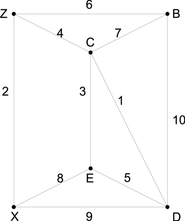
(a) Undirected (G)

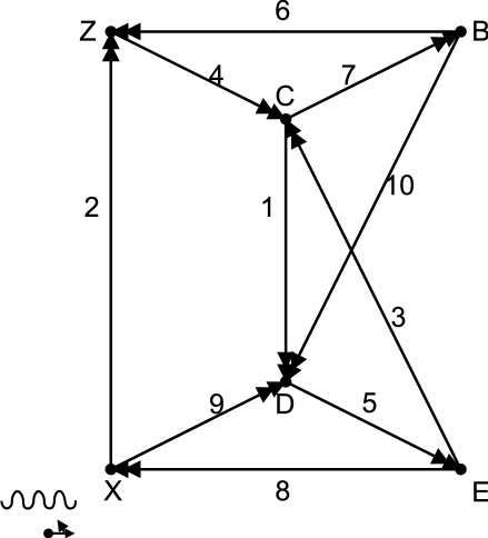
(b) Directed (G,E)

Figure 9. The graph underlying fig. 4

Two different drawings of the same (labelled) graph are shown. The first is an undirected version of the second. Moreover, since we are excluding loops and parallel or anti-parallel edges, we can identify each undirected edge in the first with a directed edge in the second. The second can be converted into fig. 4 (on page 4), using the following recipe. View the picture as a line arrangement in the Euclidean plane. Notice the choice of polar origin. Twist each edge of the graph, just a little, by moving the pointy head further away from the origin, while keeping the other end fixed. Add a pinch of imagination, and we have figure 4.

Let’s formalise that recipe, keeping the pinch of imagination down to a minimum.

We start by observing that the crucial properties of figure 4 that we care about are listed in theorem 7.1. These are the orientations of nine triangles, and the constraints on the ordering of the lines. These constraints describe a partial order, $\prec$. For now, we will ignore the triangle $\{1,5,7\}$ since it clearly plays a special role (for example, it plays no part in the proof of lemma 11.2). Each of the remaining eight triangles corresponds to one of the six vertices in the graph. Vertices $C$ and $D$, having degree 4, have two corresponding triangles.

Given any total order $<$ over $E$ extending $\prec$, then the triangles can be expressed as a subset $A$ of the $\mathcal{C}(<)$.

In order to express this, we extend the idea of the circuits corresponding to an order in the following fashion:

Definition 13.1.

Given a partial order $\prec$ over $E$, the circuits $\mathcal{C}(\prec)$ are those circuits that are circuits of $\mathcal{M}(<)$ for every total order $<$ of $E$ which extends $\prec$.

i.e.

(122) $$\mathcal{C}(\prec)=\bigcap_{<\supseteq\prec}\mathcal{C}(<)$$

For a total order $<$, definition 13.1 and equation (114) are consistent.

Definition 13.2.

A twisted graph $T=(\vec{G},G,\prec,A)$ is a directed graph $\vec{G}=(V,\vec{E})$, with $\prec$ partially ordering $E$, such that:

1. $G=(V,E)$ is the underlying simple graph of $\vec{G}$

2. $G$ is three edge connected

3. $A\subset\mathcal{C}(\prec)$

4. for every total order $<$ of $E$ extending $\prec$ there is a strong map $\mathcal{M^{*}}(\vec{G})\rightarrow\mathcal{M}(<)$.

5. $A$ can be partitioned into $\{A_{v}:v\in V\}$ with $C^{*}_{v}$ (as in equation (118)) being the conformal composition over $A_{v}$ for each $v$.

Essentially, a twisted graph is formed from the signed incidence matrix of $\vec{G}$, by taking every row with more than three entries, and splitting it into rows of $A$ (considered as a matrix), each having three entries. Every row has the form $(-,+,-)$ or $(-,+,-)$ with the rest of the entries being zero.

For example, we take the incidence matrix of fig. 9(b):

(123) $$\left(\setcounter{MaxMatrixCols}{11}\begin{smallmatrix}&(1)&(2)&(3)&(4)&(5)&(6)&(7)&(8)&(9)&(10)\\ (E)&&&-&&+&&&-&&\\ (X)&&-&&&&&&+&-&\\ (Z)&&+&&-&&+&&&&\\ (B)&&&&&&-&+&&&-\\ (C)&-&&+&+&&&-&&&\\ (D)&+&&&&-&&&&+&+\end{smallmatrix}\right)$$

and split the last two rows, because they have more than three entries, to give:

(124) $$\left(\setcounter{MaxMatrixCols}{11}\begin{smallmatrix}&(1)&(2)&(3)&(4)&(5)&(6)&(7)&(8)&(9)&(10)\\ (E)&&&-&&+&&&-&&\\ (X)&&-&&&&&&+&-&\\ (Z)&&+&&-&&+&&&&\\ (B)&&&&&&-&+&&&-\\ (C)&-&&+&&&&-&&&\\ (C^{\prime})&-&&&+&&&-&&&\\ (D)&+&&&&-&&&&+&\\ (D^{\prime})&+&&&&-&&&&&+\end{smallmatrix}\right)$$

which, with the insertion of appropriate $S^{j}_{i}$ values is $M_{8}$ from equation (100).

While we don’t exploit such a view of a twisted graph, for explanatory purposes, we express it more formally as:

Proposition 13.3.

If $T=(\vec{G},G,\prec,A)$ is a twisted graph then there is a function $v:A\rightarrow V$ such that:

1. For each $a\in A$, there is a single vertex $v(a)\in V$ incident with each of the edges in $\underline{a}$.

2. For each $e\in E$, there is some $a\in A$, with $a(e)=1$, and $e=(u,v(a))$, for some $u\in V$

3. For each $e\in E$, there is some $a\in A$, with $a(e)=-1$, and $e=(v(a),u)$, for some $u\in V$

4. For each each $e\in E$, there are $a,a^{\prime}\in A$, with $a(e)=1$ and $a(e)=-1$, and $e=(v(a^{\prime}),v(a))$.

5. Given $a_{1},a_{2}\in A$, and some $e\in E$ for which $a_{1}(e)=a_{2}(e)\neq 0$ then $v(a_{1})=v(a_{2})$.

6. If $a_{1},a_{2}\in A$ are conformal, and $\underline{a_{1}}\cap\underline{a_{2}}\neq\emptyset$ then $v(a_{1})=v(a_{2})$.

Proof.

By construction, each $a\in A$, is in some $A_{v}$. Since $C^{*}_{v}$ is the conformal composition of $A_{v}$, we have for each edge $e\in\underline{a}$ that $a(e)=C^{*}_{v}(e)$. Thus, from (118), for each edge $e\in a$, there is a $u\in V$, such that either $e=(u,v)$ and $a(e)=C^{*}_{v}(e)=1$ or $e=(v,u)$ and $a(e)=C^{*}_{v}(e)=-1$. So $v(a)=v$ is incident with each edge in $a$. If there was some other vertex also incident with each edge in $a$, then we would have three parallel edges, which we have excluded.

For the second point, we note that if $e=(u,v)$, then $C^{*}_{v}(e)=1$, and there is some $A_{v}\subset A$, such that the conformal composition over $A_{v}$ is $C^{*}_{v}$, so there is at least one $a\in A_{v}$ with $a(e)=C^{*}_{v}(e)$. By the previous paragraph, for this $a$, we have $v(a)=v$.

The third point is similar.

The fourth point is a rephrasing of the second and third points.

For the fifth point, $e=(v(a^{\prime}),v(a))$ as in the fourth point, and for the case $v(a_{1})=1$ we can, without loss of generality, take $a=a_{1}$. From the first point, $v(a_{2})$ is incident with $e$, and $a_{2}\neq a^{\prime}$ because $a_{2}(e)\neq a^{\prime}(e)$. Thus $a_{2}=a_{1}$.

The sixth point follows from the fifth by taking any $e\in\underline{a_{1}}\cap\underline{a_{2}}$. ∎

We explore the notion of twisted graphs, with the aim of deriving minimal insoluble systems from them, corresponding to constraints on line arrangements, or the realizations of rank 3 oriented matroids.

Two preliminary definitions:

Definition 13.4.

A directed graph $\vec{G}$ can be twisted if there is a twisted graph $(\vec{G},G,\prec,A)$, for some $A$, and $\prec$.

Definition 13.5.

A simple graph $G$ can be twisted if there is some orientation $\vec{G}$ of $G$, such that $\vec{G}$ can be twisted.

We start by showing that there are infinitely many twisted graphs. Given the requirement for there to be the strong map, we wish to find a totally cyclic orientation of $G$.

Proposition 13.6.

Given a three-edge connected simple graph $G$, then there is a totally cyclic directed graph $\vec{G}$ with underlying graph $G$.

Proof.

Arbitrarily direct edge each of $G$ to get $\vec{G_{0}}$. Take the oriented matroid $\mathcal{M}=\mathcal{M}(\vec{G_{0}})$. Take an arbitrary maximal vector $v$ of $\mathcal{M}$. Reorient $\mathcal{M}$ so that $v$ is positive. Apply the same reorientation to $\vec{G_{0}}$ to get $\vec{G}$. ∎

Lemma 13.7.

Every simply three-edge connected, totally cyclic, directed graph $\vec{G}$, can be twisted.

Proof.

From corollary 12.7 we find a total order $<$ over $E$, with the strong map $\mathcal{M^{*}}(\vec{G})\longrightarrow\mathcal{M}(<)$. For every $v\in V$, $C^{*}_{v}$ is a signed minimal cut of $\vec{G}$, and hence a cocircuit of $\mathcal{M}(\vec{G})$, i.e. a circuit of $\mathcal{M^{*}}(\vec{G})$. By the strong map, $C_{v}$ is a vector of $\mathcal{M}(<)$, and hence a conformal composition of some set of circuits $A_{v}$ of $\mathcal{M}(<)$. We put $A=\bigcup_{v\in V}A_{v}$, and we have a twisted graph, with a total order. ∎

Corollary 13.8.

Every three-edge connected, simple graph $G$ can be twisted.

The definition of twisted graph permits adding more triangles to $A$ than is strictly needed (for some vertices incident with more than four edges). So the following definition is helpful:

Definition 13.9.

A twisted graph $T=(\vec{G},G,\prec,A)$ is irredundant if:

• for all proper subsets $A^{\prime}\subsetneq A$, then $T^{\prime}=(\vec{G},G,\prec,A)$ is not a twisted graph.

• for all partial orders $\prec^{\prime}\subsetneq\prec$, then $T^{\prime}=(\vec{G},G,\prec^{\prime},A)$ is not a twisted graph.

13.1. Why the strong maps?

Definition 13.2 requires the existence of at least one strong map. However, the results in this paper do not depend on that condition, nor even the potentially weaker condition that $\vec{G}$ be totally cyclic.

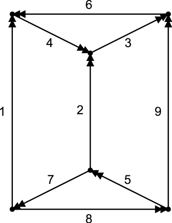
Figure 10. Should this be a twisted graph?

The motivation for this condition is to prevent graphs like in figure 10, from being twisted. The numbering in that figure shows a potential ordering. This satisfies the conclusions of proposition 13.3, and definition 13.2 without the strong map constraint. The positive cut of size three prevents there from being a strong map.

Currently, I think the various conjectures I make in the subsequent sections are more plausible with the strong map condition. This is the motivation.

13.2. Matrices, Realisations and Twisted Graphs

Of course, our interest in twisted graphs is because of their relationship to matrices that express conditions on line arrangements. A twisted graph is realized by a line arrangement $(\mathcal{L}_{e})_{e\in E}$, with a polar frame of reference, if for every $a=(\{e,f\},\{g\})\in A$, the triangle $\{L_{e},L_{f},L_{g}\}$ is positively oriented, and likewise for every $(\{e\},\{f,g\})\in A$ there is a negatively oriented triangle.

To express this in the fashion of the previous sections, given a twisted graph $T$, we consider a vector of angles $\boldsymbol{\theta}$ indexed by $E$, and construct a $|A|$ by $|E|$ matrix $\Sigma=\Sigma(T)$ with entries being either $0$ or $\sin(\theta_{f}-\theta_{e})$ or $-\sin(\theta_{f}-\theta_{e})$ with $e,f\in E$ and $e\prec f$.

The actual entries are given, for each $a\in A$ and $e\in E$ by:

(125) $$\Sigma_{a,e}=\begin{cases}0&e\notin a\\ a(e)\sin(\theta_{e}^{\prime\prime}-\theta_{e}^{\prime})&\underline{a}=\{e,e^{\prime},e^{\prime\prime}\},e^{\prime}\prec e^{\prime\prime}\end{cases}$$

So as we have seen, there is a $T$ corresponding to figure 9(b), with $\Sigma(T)$ being a matrix consisting of the rows of $M_{8}$, equation (100), in some order.

This matrix can be understood either as a matrix of formal expressions over $\boldsymbol{\theta}$ or as a matrix over $\mathbb{R}$, given specific values of $\boldsymbol{\theta}$. So that we can compute signs of determinants, we restrict the values of interest, to those that respect $\prec$.

Definition 13.10.

A vector of real numbers $\boldsymbol{\theta}\in\mathbb{R}^{E}$ respects $\prec$, when:

• For all $e\in E$, $0<\theta_{e}<180$

• For all $e,f\in E$, if $e\prec f$ then $\theta_{e}<\theta_{f}$.

Then a solution in $\boldsymbol{\theta},\boldsymbol{r}\in\mathbb{R}^{E}$, with $\boldsymbol{\theta}$ respecting $\prec$, for the system:

(126) $$\Sigma(T)\boldsymbol{r}>0$$

provides polar coordinates of a line arrangement realizing $T$. If the solution in $\boldsymbol{r}$ is not positive, then the arrangement can still be drawn, interpreting negative values for any $r_{e}$ as in the opposite direction to positive values. Moving the polar origin will then give a solution that is all positive. More formally, we can convert the first set of coordinates into homogeneous coordinates and then use lemma 6.1 to find true polar coordinates. So, without loss of generality, we can take $\boldsymbol{r}>0$.

We have seen in lemma 11.1, that for one twisted graph $T$, and for some $\boldsymbol{\theta}$, that $\Sigma(T)$ is a minimal insoluble system. We ask whether this is generally the case.

Conjecture 13.11.

For every twisted graph $T$, there is some $\boldsymbol{\theta}$ respecting $\prec$, for which $\Sigma(T)\boldsymbol{r}>0$ is not soluble.

To simplify statements of such conjectures and theorems, we introduce the term constraining:

Definition 13.12.

A twisted graph is constraining if there is some $\boldsymbol{\theta}$ respecting $\prec$, for which $\Sigma(T)\boldsymbol{r}>0$ is not soluble, and for which $\Sigma(T)\boldsymbol{r}=0$ has a nontrivial solution.

Conjecture 13.11 can be strengthened to

Conjecture 13.13.

Every irredundant $\prec$-minimal twisted graph $T=(\vec{G},G,\prec,A)$ is constraining.

where $\prec$-minimal is defined as:

Definition 13.14.

A twisted graph $T=(\vec{G},G,\prec,A)$ is $\prec$-minimal if for each $e\in E$, there is no $A^{\prime}$ such that $T=(\vec{G}\setminus e,G\setminus e,\prec\setminus e,A^{\prime})$ is a twisted graph.

If these conjectures are true, then we would also have (by lemma 13.7), the weaker:

Conjecture 13.15.

For every minimal simply three edge connected, totally cyclic directed graph $\vec{G}$, there is a total order $<$, and a constraining twisted graph, $T=(\vec{G},G,<,A)$.

and the, weaker still

Conjecture 13.16.

For every minimal three edge connected simple graph $G$, there is a directed graph $\vec{G}$, total order $<$, and a constraining twisted graph, $T=(\vec{G},G,<,A)$.

We will find an initial class of constraining twisted graphs, including all three edge connected cubic graphs.

We will see that the somewhat surprising proofs of lemmas 11.2 and 11.4 are general, and not sporadic facts about the non-Pappus arrangement.

14. A Representation of $\mathcal{M}(<)$ and $\mathcal{M}(\vec{G})$

We continue, our study of twisted graphs, by a simultaneous representation of both the oriented matroids of interest, within the vector space in $\mathbb{R}^{n}$, where $n=|E|$. We identify $E$ with the numbers $1\ldots n$, such that $e_{i}<e_{j}$ if and only if $i<j$. We take $\boldsymbol{\theta}$ to be an increasing sequence of values in $(0,180)^{n}$, rather than a sequence of formal variables: although we will once or twice, consider the effect of modifying some of these values, we are, in the main, considering $\boldsymbol{\theta}$ as a given vector.

Each circuit and cocircuit of $\mathcal{M}(<)$ is represented as a non-zero point in $\mathbb{R}^{n}$. Each vector and covector are represented by the convex cone formed from non-negative combinations of the rays corresponding to the conforming circuits or cocircuits. Thus, a circuit, when considered as a vector, is represented by a ray from the origin through the point corresponding to the circuit.

The strong map from $\mathcal{M^{*}}(\vec{G})$ to $\mathcal{M}(<)$, then allows each of the cocircuits of $\mathcal{M}(\vec{G})$ to be represented by the cone representing it when considered as a vector of $\mathcal{M}(<)$.

For circuits of the form $+C_{i,j,k}=(\{i,k\},\{j\})$, with $1\leq i<j<k\leq n$, the corresponding point is given by:

(127) $$\widehat{+C_{i,j,k}} =\begin{pmatrix}x_{1}&x_{2}&\cdots&x_{n}\end{pmatrix}$$

(128) $$x_{h} =\begin{cases}\sin(\theta_{k}-\theta_{j})&h=i\\ -\sin(\theta_{k}-\theta_{i})&h=j\\ \sin(\theta_{j}-\theta_{i})&h=k\\ 0&\text{otherwise}\end{cases}$$

We represent the opposite circuits by the opposite points.

For cocircuits of the form $+C^{*}_{i}=(\{j:1\leq j<i\},\{j:n\geq j>i\})$, with $1\leq i\leq n$, the corresponding point is given by

(129) $$\widehat{+C^{*}_{i}}=\begin{pmatrix}S^{i}_{1}&S^{i}_{2}&\cdots&S^{i}_{n}\end{pmatrix}$$

Again, the opposites are represented by the opposite points.

Immediately from proposition 8.4, we have the following:

Proposition 14.1.

For any circuit $C\in\mathcal{C}(<)$ and any cocircuit $C^{*}\in\mathcal{C^{*}}(<)$, $\hat{C}\perp\hat{C^{*}}$.

We can represent any set $X$ of circuits or cocircuits as a non-negative sum of the representations of its members:

(130) $$\hat{X}=\left\{\sum_{x\in X}\lambda_{x}\hat{x}:\lambda_{x}\geq 0\right\}$$

so that if $X$ is symmetric (i.e. $x\in X$ if and only if $-x\in X$), $\hat{X}$ is a vector space.

The basic structure of the representation is then captured in the following proposition:

Proposition 14.2.

With $\hat{}$ as defined above:

1. $\widehat{\mathcal{C}(<)}\perp\widehat{\mathcal{C^{*}}(<)}$

2. $\widehat{\mathcal{C}(<)}$ has rank $n-2$.

3. $\widehat{\mathcal{C^{*}}(<)}$ has rank $2$.

Proof.

The first point follows from the previous proposition.

It then suffices to show $n-2$ independent members of $\widehat{\mathcal{C}(<)}$, and $2$ independent members of $\widehat{\mathcal{C^{*}}(<)}$, since $\operatorname{rank}\widehat{\mathcal{C}(<)}+\operatorname{rank}\widehat{\mathcal{C^{*}}(<)}\leq n$.

The set $\{\widehat{C_{i,n-1,n}}:1\leq i\leq n-2\}$ is independent, by considering the first $n-2$ coordinates.

The set $\{\widehat{C^{*}_{1}},\widehat{C^{*}_{2}}\}$ is independent by considering the first $2$ coordinates. ∎

For a partial order $\prec$, and for any $C\in\mathcal{C}(\prec)$, $\hat{C}$ is independent of the total order $<$ extending $\prec$ used, so that $\hat{C}$ and $\widehat{\mathcal{C}(\prec)}$ are well-defined. In addition, $\widehat{\mathcal{C}(\prec)}\subset\widehat{\mathcal{C}(<)}$, so that:

Proposition 14.3.

For a partial order, $\widehat{\mathcal{C}(\prec)}$ has rank at most $n-2$.

We tie this back in with the previous section:

Proposition 14.4.

If $T=(\vec{G},G,\prec,A)$ is a twisted graph, then $\Sigma(T)=\hat{A}$.

15. Twisted Graphs with Simplexes

The key interesting property of the twisted graph that we studied in section 11, is that the corresponding matrix $\Sigma$ contains a simplex. We will now study such twisted graphs, generalising the treatment in section 11, and providing a condition sufficient for a twisted graph to have such a simplex. This provides an alternative proof of the main theorem.

Definition 15.1.

A twisted graph $T=(\vec{G},G,\prec,A)$ is simplicial on $F\subset E$, if the submatrix of the system $\Sigma=\Sigma(T)$ formed from the columns indexed by $F$ is a simplex, for every $\boldsymbol{\theta}$ respecting $\prec$.

We note that in this case $|F|=|A|-1$.

As an example, consider the twisted graph $T$ corresponding to $M_{8}$, equation (100): lemma 11.1 shows that $T$ is simplicial on $\{2,3,4,6,8,9,10\}$.

If there is a linear dependency between the rows of $\Sigma$ then there is only one (up to multiplication) and it is the unique positive dependency (restricted to $F$), provided by the simplex. Thus, rank $\Sigma$ is either $|A|$ or $|A|-1$. In the example, we saw that which of these held, depends on the choice of $\boldsymbol{\theta}$. Now, $\Sigma$ is also a set of $|A|$ vectors from $\widehat{\mathcal{C}(\prec)}$, which has rank at most $|E|-2$, hence:

Proposition 15.2.

For a simplicial twisted graph $T=(\vec{G},G,\prec,A)$, $|A|\leq|E|-2$.

Now, consider the set $F^{c}=E\setminus F$. This has at least three members. We want to look at the restriction of $\widehat{\mathcal{C}(\prec)}$ to $F^{c}$, i.e. those which are zero on all members of $F$. In the conditions on the main theorem, we saw that the partial order being used totally orders $F^{c}$. This motivates:

Definition 15.3.

A twisted graph $T=(\vec{G},G,\prec,A)$ is strictly simplicial if it is simplicial on $F$ and $E\setminus F$ is totally ordered by $\prec$.

In such a case, taking $<$ as a total order extending $\prec$:

(131) $$\widehat{\mathcal{C}(\prec)}|_{F^{c}} =\widehat{\mathcal{C}(<)}|_{F^{c}}$$

(132) $$=\widehat{\mathcal{C}(<)}\cap\mathbb{R}^{F^{c}}$$

(133) $$=\{c\in\widehat{\mathcal{C}(<)}:c(f)=0\text{ for all }f\in F\}$$

(134) $$=\{c\in\mathbb{R}^{F^{c}}:c\perp\widehat{\mathcal{C^{*}}(<)}\}$$

the last of these, follows from proposition 14.2, and we conclude:

Proposition 15.4.

$\widehat{\mathcal{C}(\prec)}|_{F^{c}}$ has rank $|F^{c}|-2$.

So for a strictly simplicial twisted graph, we can take a basis $\{b_{1},b_{2},\ldots b_{k}\}$ for $\widehat{\mathcal{C}(\prec)}|_{F^{c}}$, with $k=|F^{c}|-2=|E|-|F|-2$. Thus $|A|+k=|E|-1$. Moreover, $\Sigma\cup\{b_{1},b_{2},\ldots b_{k}\}\subset\widehat{\mathcal{C}(\prec)}$, and $|\Sigma\cup\{b_{1},b_{2},\ldots b_{k}\}|=|E|-1>|E|-2\geq\operatorname{rank}\widehat{\mathcal{C}(\prec)}$. Thus, there is a linear dependency amongst $\Sigma\cup\{b_{1},b_{2},\ldots b_{k}\}$.

Also, we can choose the basis such that, for each $i$, $b_{i}=\widehat{C_{i}}$, for some circuit $C_{i}$ in $\mathcal{C}(\prec)$, with $\underline{C_{i}}\subset F_{c}$. By taking $B$ as an appropriate subset (not necessarily proper) of $\{C_{1},C_{2},\ldots C_{k}\}$, we have the following:

Lemma 15.5.

For a twisted graph $T=(\vec{G},G,\prec,A)$, strictly simplicial on $F$, there is some subset $B\subset\mathcal{C}(\prec)\setminus F$, such that there is a homogeneously unique linear dependency $\Lambda$ in $\widehat{A\cup B}$

Proof.

If $\widehat{A}$ has a linear dependency, take $B=\emptyset$, any linear dependency of $\widehat{A}$, is also a linear dependency of the rows of the simplex, and hence homogeneously unique.

Otherwise choose a basis $B_{0}$ for $\widehat{\mathcal{C}(\prec)}|_{F^{c}}$. By considering the rank, we have that $A\cup B_{0}$ is a linearly dependent set, hence, there is some $B\subset B_{0}$, such that $\widehat{A\cup B}$ is a minimal independent set, and has a homogeneously unique linear dependency. ∎

Lemma 15.6.

In the previous lemma, $B$ can be chosen such that $\Lambda>0$.

Proof.

Since $\widehat{B}$ is a linearly independent set, there is some some $a\in A$, with $\lambda_{a}\neq 0$. By multiplying by $-1$ if necessary, $\lambda_{a}>0$. Since $\widehat{B}\subset\mathbb{R}^{F^{c}}$, $\Lambda$ gives a linear dependency for the simplex indexed by $F$, thus $\lambda_{a^{\prime}}>0$ for all $a^{\prime}\in A$. For each $b\in B$, if $\lambda_{b}<0$ we can replace $b$ with $-b$ to get the desired result. ∎

Combining the previous lemma with Carver’s theorem, we get:

Theorem 15.7.

For a strictly simplicial twisted graph $T=(\vec{G},G,\prec,A)$, for every $\boldsymbol{\theta}$ respecting $\prec$, there is some set $B$ of circuits from $\mathcal{C}(\prec)$ such that $\widehat{A\cup B}.\mathbf{r}>0$ is a minimal insoluble system.

Proof.

The previous lemma furnishes a positive linear dependency, showing from theorem 9.5, that the system is insoluble. If there were some proper insoluble subsystem, then the same theorem would furnish a different positive linear dependency, contradicting the uniqueness of the previous lemma. ∎

As in section 11, this system can be analysed in terms of determinants of submatrices of $\widehat{A\cup B}$ to give a set of equations and inequalities that are sufficient for a system to be insoluable. By allowing the $\boldsymbol{\theta}$ to vary, we can find conditions sufficient for the system $\widehat{A\cup B}.\mathbf{r}>0$ to be soluble, i.e. for every subset of $B$, the conditions for insolubility do not hold. We conjecture that for any set $B$ chosen as in lemma 15.6, with some specific $\boldsymbol{\theta}$ respecting $\prec$, such that the system $\widehat{A\cup B}.\mathbf{r}>0$ is not soluble, there is some other $\boldsymbol{\theta^{\prime}}$ which respects $\prec$ for which the system is soluble. This would allow us to represent any simplicial twisted graph as a line arrangement, like figure 4, with some constraint on the angles in that arrangement. Further investigation of this conjecture may depend on converting the various constraints, which all amount to constraints on the signs of differences of pairs of sums of products of sines, into normal form, using section 10, and showing that there is a simultaneous solution.

15.1. Maximal Simplicial Twisted Graphs

We investigate one case further, the easiest, when $|A|=|E|-2$, so that $k=0$ or $k=1$. The analogue of lemma 11.1, requires us to consider the signs of the determinants of three matrices. These signs are all covariant, or contravariant. Precisely which depends on the detail of the relative ordering of the members of $F_{c}$ within $E$, since odd permutations cause sign changes of determinants.

Lemma 15.8.

For a twisted graph $T=(\vec{G},G,\prec,A)$, strictly simplicial on $F$, with $|F|=|E|-3$, then there is a signed set $X$ with $\underline{X}=F_{c}$, such that for each $\boldsymbol{\theta}$ respecting $\prec$, there is a sign $\sigma(\boldsymbol{\theta})\in\{-1,0,+1\}$, and for each $x\in E\setminus F$, the matrix formed from the $F\cup\{x\}$ columns of $\Sigma$ has determinant with sign $X(x)\sigma(\boldsymbol{\theta})$.

Proof.

Given a specific $\boldsymbol{\theta}$ either $\operatorname{rank}\Sigma=|A|-1$ or $\operatorname{rank}\Sigma=|A|$. In the first case, each of the three matrices is singular, and $\sigma(\boldsymbol{\theta})=0$.

In the second case, we write $F_{c}=\{x_{1},x_{2},x_{3}\}$ with $x_{1}\prec x_{2}\prec x_{3}$; we write $C=(\{x_{1},x_{3}\},\{x_{2}\})$. We find the circuit $C^{\prime}$ and $B=\{C^{\prime}\}$ satisfying lemma 15.6. Either $C^{\prime}=C$ or $C^{\prime}=-C$.

We set:

(135) $$\sigma(\boldsymbol{\theta})=\begin{cases}1&C^{\prime}=C\\ -1&C^{\prime}=-C\end{cases}$$

For each $x\in F_{c}$, the positive dependency $\Lambda$ from that lemma is also a positive dependency of the $|A|$ by $|A|+1$ submatrix $\Sigma^{\prime}$ of $\widehat{A\cup\{C^{\prime}\}}$, formed from the columns $F\cup\{x\}$. Moreover, it is unique, because the last row, $\widehat{C^{\prime}}$, of the submatrix, is zero on $F$, and has only the one non-zero entry at $x$, and we know that the other rows and columns have a unique positive dependency, being a simplex.

Thus, $\Sigma^{\prime}$ is a simplex, and the signs of the subdeterminants alternate. The signs of the first $|A|$ subdeterminants are given by the sign of $C^{\prime}(x)$, the position of $x$ with respect to $F$ (and hence the sign of the permutation to move $x$ to the final column of the submatrix), and the sign of the corresponding subdeterminant in the simplex from $\hat{A}$ on $F$. We choose each $X(x)$ to satisfy the lemma for some particular $\boldsymbol{\theta}$. For a different $\boldsymbol{\theta}$, where we also find $C^{\prime}=C$ none of the signs in the derivation change, so that the same $X$ satisfies. On the other hand, if we find $C^{\prime}=-C$, the sign of $C^{\prime}(x)$ has changed, and so has the sign of $\sigma(\boldsymbol{\theta})$, so that once again $X$ satisfies the lemma. ∎

We conjecture that in all such cases, $\sigma$ is surjective, which allows us to draw a line arrangement corresponding to both variations of $A$ and $C$ or $-C$, and a third arrangement in which each $a\in A$ corresponds to a point in the drawing.

Theorem 15.9.

For a twisted graph $T=(\vec{G},G,\prec,A)$, simplicial on $F$, with $E=F\mathaccent 0{\cdot}\cup\{x_{1},x_{2},x_{3}\}$, with $x_{1}\prec x_{2}\prec x_{3}$, and $C$ being either $(\{x_{1},x_{3}\},\{x_{2}\})$ or its opposite, then there is a sign $\sigma_{C}\in\{1,-1\}$, such that $\widehat{A\cup\{C\}}.\mathbf{r}>0$ is soluble for $\boldsymbol{\theta}$ respecting $\prec$ if and only if the sign of the determinant of the square submatrix of $\hat{A}$ on columns $F\cup\{x_{1}\}$ is $\sigma_{C}$. Moreover, $\sigma_{-C}=-\sigma_{C}$.

Proof.

We suppose a specific $\boldsymbol{\theta}$, and taking $\sigma(\boldsymbol{\theta})$ as in the previous lemma, if the specified determinant is zero, then $\sigma(\boldsymbol{\theta})=0$, and all the determinants on columns $F\cup\{x_{i}\}$ are also zero, and hence not equal to $\sigma_{C}$, moreover, the system is insoluble, so this theorem is satisfied.

Otherwise, whether $\widehat{A\cup\{C\}}$ has a simplex or not on $F\cup\{x_{1}\}$ depends only on the sign of $C(x_{1})$, and the sign of the determinant of the square submatrix specified, since $\widehat{A}$ has a simplex on $F$, and $C$ is zero on $F$. Thus we choose $\sigma_{C}$ to be the sign such that this is not a simplex.

Since $\sigma_{C}$ depends on $C(x_{1})$, which is not zero, we have that $\sigma_{-C}=-\sigma_{C}$. ∎

15.2. Positive Sequences

So, given that simplicial twisted graphs have this interesting property, how can we easily tell if a twisted graph is simplicial, other than the laborious computation of determinants that we did in section 11. If $G$ is cubic, then a very quick glance at the matrix, is sufficient to see that any spanning tree of $G$ gives a simplex, for example, we consider an orientation of $K_{4}$, to get:

(136) $$\begin{pmatrix}+&-&+&&&\\ -&&&+&-&\\ &+&&-&&+\\ &&-&&+&-\end{pmatrix}$$

This functions both as the incidence matrix of the directed graph, and the matrix corresponding to the twisted graph, if we interpret the signs as representing signed values $S^{j}_{i}$. If we consider the spanning tree formed from the first three edges, we see that in any linear dependency $\Lambda$ amongst the rows of the 3 by 4 submatrix, the second, third and fourth rows must each have the same sign as the first, by considering the first, second and third columns respectively. For each, the ratio between the values of $\lambda_{i}$ is the inverse of the ratio of the entries in the matrix. Since the submatrix has more rows than columns, there must be at least one linear dependency. Since the signs of each row are the same as the first row, this is a positive linear dependency. Since the ratios are fixed, it is homogenously unique.

We can generalise this argument as follows.

Definition 15.10.

Given a twisted graph $T=(\vec{G},G,\prec,A)$, then a positive sequence for $T$ on $F$ is an ordering $A=\{a_{1},a_{2},\ldots a_{m}\}$ and an ordered subset of $F\subset E$, $F=\{f_{2},\dots f_{m}\}$ with $m=|A|$, such that for each $j$, $2\leq j\leq m$:

• $a_{j}(f_{j})\neq 0$.

• For all $i>j$, $a_{i}(f_{j})=0$.

• For all $i<j$, $a_{i}(f_{j})\in\{0,-a_{j}(f_{j})\}$.

Note, the absence of $f_{1}$.

The ordering $f_{2},f_{3}\ldots$ is not usually related to the order $\prec$.

Proposition 15.11.

If $G$ is cubic, and has a spanning tree $F$, then for any twisted graph $T=(\vec{G},G,<,A)$ has a positive sequence on $F$.

Proof.

Consider any sequence such that the initial subsequences form a connected subgraph of $F$. ∎

Proposition 15.12.

For any positive sequence as in definition 15.10, for every $2\leq j\leq m$, there is an $i<j$, such that $a_{i}(f_{j})=-a_{j}(f_{j})\}$.

Proof.

From proposition 13.3 there is some $a_{i}$ such that $a_{i}(f_{j})=-a_{j}(f_{j})$. From the definition of positive sequence, we then have $i<j$. ∎

We now show that a twisted graph with a positive sequence is simplicial.

Theorem 15.13.

A twisted graph $T=(\vec{G},G,\prec,A)$, with a positive sequence is simplicial.

Proof.

Take $A=\{a_{1},a_{2},\ldots a_{m}\}$ and $F=\{f_{2},f_{3},\dots f_{m}\}\subset E$, as the positive sequence.

Consider the submatrix of $\hat{A}$ formed from the columns corresponding to $F$. There is at least one linear dependency between its rows, since it has more rows than columns, call this $\Lambda=\lambda_{i}$, where the subscripts correspond to the positive sequence on $A$.

From the definition, for each $j>1$, we have

(137) $$\sum_{i=1}^{m}\lambda_{i}\hat{a_{i}}(f_{j}) =0$$

(138) $$\sum_{i=1}^{j}\lambda_{i}\hat{a_{i}}(f_{j}) =0$$

(139) $$\lambda_{j} =-\sum_{i=1}^{j-1}\lambda_{i}\hat{a_{i}}(f_{j})/\hat{a_{j}}(f_{j})$$

By multiplying by a constant we can assume that the first non-zero value in $\Lambda$ is 1.

Suppose that the first non-zero value is $\lambda_{j}$ with $j>1$. Then equation (139) gives a contradiction. Thus $\lambda_{1}=1$.

Now, suppose the first non-positive value is $\lambda_{j}$. Then equation (139) gives a contradiction. Moreover, the same equation shows that the positive dependency is unique. Thus the matrix is a simplex, and we are done. ∎

We can now give a shorter proof for the main theorem. While the ground work for this proof was extensive, the style of the proof can be reused, like final polynomials, but the positive sequence is easier to verify. If using this within a non-stretchability proof, the steps corresponding to lemma 8.5 are also required.

Second proof of theorem 7.1.

Consider the twisted graph $T$ corresponding to figure 9(b), and $M_{8}$ of (100). We can construct a positive sequence from the eight rows in order, and columns $\{8,2,6,3,4,9,10\}$. Hence, $T$ is simplicial. Since $\{1,5,7\}$ is totally ordered by the specified partial order, $T$ is strictly simplicial. We apply theorem 15.9, looking at figure 4. This shows that the system corresponding to (99) is soluble, when $\boldsymbol{\theta}=(42,20,62,80,120,98,158,125,149,170)$. The angles are approximate, measured from the figure.

The determinant of the 8-by-8 submatrix on columns $\{2,3,4,5,6,8,9,10\}$, is given by $d_{5}$, equation (104). In figure 4 this evaluates to approximately $-0.17$, which is negative, hence the value $\sigma$ in theorem 15.9 is -1. Factoring out $S^{7}_{1}S^{7}_{1}S^{5}_{1}$ completes the proof. ∎

A variant of this proof more suited to automation would consider one of the other determinants to provide $\sigma$, rather than a drawing.

16. Pseudoline Stretching and Further Directions

We have studied the realizability of a particular oriented matroid by considering only some of the values from its chirotope. This, of course, is also the case with the method of final polynomials.

This suggests that we may fruitfully study partial oriented matroids. An approach to axiomatising them for the rank 3 case, is to fix a line at infinity, and then provide an abstraction of a Euclidean line arrangement, in terms of the ordering of the angles of the lines, and the orientation (positive, cocurrent or negative) of some of the sets of three lines. We sketch such an approach.

16.1. Euclidean Arrangements

We define a combinatoric object, a Euclidean arrangement, $\mathbf{\mathcal{A}}$ over a set $X$, preordered by $\preccurlyeq$, in terms of a set of ordered triples $A\subset X^{3}$.

Definition 16.1.

A set of triples $A$ is alternating when $(x,y,z)\in A$ if and only if $(y,z,x)\in A$.

This corresponds to the alternating nature of a chirotope. We record negative values from the chirotope with an odd permutation:

Definition 16.2.

If $A$ is a set of triples, then $-A$ is given by:

(140) $$-A=\left\{(y,x,z):(x,y,z)\in A\right\}$$

We also write:

(141) $$A^{0} =A\cap-A$$

(142) $$A^{+} =A\setminus A^{0}$$

(143) $$A^{-} =-A\setminus A^{0}$$

The preorder $\preccurlyeq$ is not strict, so it is helpful to define:

Definition 16.3.

$x,y\in X$ are parallel, if $x\preccurlyeq y$ and $y\preccurlyeq x$.

We write $x\parallel y$ in this case, and $x\prec y$ to mean: $x\preccurlyeq y$ but not $y\preccurlyeq x$. We also use $\parallel$ and $\prec$ to mean the corresponding subsets of $X^{2}$.

Definition 16.4.

Given a set $X$, a transitive and reflexive relation $\preccurlyeq$ over $X$, and an alternating set of triples $A$ from $X$, we can form the Euclidean arrangement $\mathbf{\mathcal{A}}=\left(X,\preccurlyeq,A\right)$, when:

A1:

For all $(x,y,z)\in A$, either $x\preccurlyeq y$ or $y\preccurlyeq x$.

A2:

For all $x,y\in X$ with $x\preccurlyeq y$ then $(x,x,y),(x,y,y)\in A$.

A3:

If $(x,y,z)\in A$ and $x\parallel y\parallel z$ then $(y,x,z)\in A$.

A4:

Each increasing sequence in $X^{4}$ is monotonic, (see definition 16.6).

The notion of monotonic used in the above definition is a variation of that from [Felsner and Weil, 1999]. It corresponds to the observation that given four pseudolines, $\{a,b,c,d\}$, if both $\{a,b,c\}$ and $\{a,b,d\}$ are coincident, then so are all four lines, and more generally to axiom B2, from [Björner et al., 1999] page 126, abstracting the Grassmann-Plücker relations. We use the following subscript conventions, with $i$ from 1 to 4: $x_{i}$ is a $\preccurlyeq$-ordered sequence of elements of $X$; $t_{i}$ is the three element subsequence of $(x_{1},x_{2},x_{3},x_{4})$ excluding $x_{i}$; $s_{i}$ is the three element subsequence of $(t_{1},t_{2},t_{3},t_{4})$ excluding $t_{i}$. In full:

(144) $$t_{1} =(x_{2},x_{3},x_{4}) t_{2} =(x_{1},x_{3},x_{4})$$

$$t_{3} =(x_{1},x_{2},x_{4}) t_{4} =(x_{1},x_{2},x_{3})$$

$$s_{1} =(t_{2},t_{3},t_{4}) s_{2} =(t_{1},t_{3},t_{4})$$

$$s_{3} =(t_{1},t_{2},t_{4}) s_{4} =(t_{1},t_{2},t_{3})$$

Definition 16.5.

For a preorder $\preccurlyeq$ a sequence $(x_{1},x_{2},\ldots,x_{k})\in X^{k}$ is $\preccurlyeq$-increasing if $x_{i}\preccurlyeq x_{i+1}$, for each $i$ from 1 to $k-1$.

In an arrangement $\mathbf{\mathcal{A}}$, a sequence is increasing if it is $\preccurlyeq$-increasing.

We note that both a sequence and a proper permutation of the same sequence can be increasing, since two or more elements may be parallel. We wish to constrain the triangles formed by an increasing sequence of four elements.

Definition 16.6.

In an arrangement $\mathbf{\mathcal{A}}$, an increasing sequence $(x_{1},x_{2},x_{3},x_{4})$ is monotonic, when, with $t_{j}$ and $s_{k}$ as in (144), for every$1\leq i,j\leq 4$: if $s_{i}\in(A\times-A\times A)\cup(-A\times A\times-A)$ then either $t_{j}\in A\cap-A$ or $x_{i}\parallel x_{j}$.

When $A\cup-A=X^{3}$ this is a cryptomorphic form of the normal axioms for an acyclic rank 3 oriented matroid over $X\cup\{\omega\}$, where $\omega$ corresponds to the line at infinity, given by $\preccurlyeq$. This motivates:

Definition 16.7.

An arrangement is complete if $A\cup-A=X^{3}$.

The advantage of this axiomatization is that it does not require complete information about the oriented matroid, but only some of the orientations. Thus, it can be used to represent the partial arrangements such as that in theorem 7.1. Informally, it amounts to permitting a chirotope $\chi$ to take values in $\left\{+1,0,-1,\ast\right\}$, where $\ast$ means ‘unknown’, and distinguishing a simple member $\omega$ of the ground set $E$, such that if $\chi(a,b,c)\neq\ast$ then $\chi(\omega,a,b)\neq\ast$.

This allows us to relate the problem of oriented matroid realizability to Ringel’s conjecture.

We need an appropriate notion of subarrangement, which we define in terms of homomorphisms:

Definition 16.8.

A homomorphism $\phi$ from an arrangement $\mathbf{\mathcal{A}}=(X,\preccurlyeq_{A},A)$ to an arrangement $\mathbf{\mathcal{B}}=(Y,\preccurlyeq_{B},B)$, is a function $\phi:X\rightarrow Y$ such that $\phi(\prec_{A})\subset\prec_{B}$, $\phi(\parallel_{A})\subset\parallel_{B}$ and $\phi(A^{+})\subset B^{+}$, $\phi(A^{0})\subset B^{0}$.

Leading, perhaps, to:

Definition 16.9.

An arrangements $\mathbf{\mathcal{A}}=(X,\preccurlyeq_{A},A)$ is a subarrangement of $\mathbf{\mathcal{B}}=(Y,\preccurlyeq_{B},B)$, if there is a function $\phi:X\rightarrow Y$, such that, for every minimal complete arrangement $\mathbf{\mathcal{C}}=(Y,\preccurlyeq_{C},C)$ extending $\mathbf{\mathcal{B}}$, i.e. $\preccurlyeq_{B}\subset\preccurlyeq_{C}$ and $B\subset C$, $\phi$ extends to a homomorphism $\phi:\mathbf{\mathcal{A}}\rightarrow\mathbf{\mathcal{C}}$.

In this case, we write $\phi:\mathbf{\mathcal{A}}\hookrightarrow\mathbf{\mathcal{B}}$, and $\mathbf{\mathcal{A}}\lesssim\mathbf{\mathcal{B}}$.

We extend definition 13.10

Definition 16.10.

A vector of real numbers $\boldsymbol{\theta}\in\mathbb{R}^{X}$ respects $\preccurlyeq$, when:

• For all $e\in X$, $0<\theta_{e}<180$

• For all $e,f\in X$, with $e\prec f$, $\theta_{e}<\theta_{f}$.

• For all $e,f\in X$, with $e\parallel f$, $\theta_{e}=\theta_{f}$.

A realization of an arrangement $\mathbf{\mathcal{A}}=(X,\preccurlyeq_{A},A)$ is defined in terms of polar coordinates.

Definition 16.11.

A realization of an arrangement $\mathbf{\mathcal{A}}=(X,\preccurlyeq_{A},A)$ is a pair of vectors $\boldsymbol{r},\boldsymbol{\theta}\in\mathbb{R}^{X}$, such that:

• $\boldsymbol{\theta}$ respects $\preccurlyeq$.

• For all $t=\{x,y,z\}\in A\cup-A$, with $x\preccurlyeq y\preccurlyeq z$:

  • if $t\in A^{0}$ equation (8) holds.

  • if $t\in A^{+}$ inequality (9) holds.

  • if $t\in A^{-}$ inequality (10) holds.

For complete arrangements, this is the same notion as oriented matroid realizability; with a coordinate transform from homogeneous coordinates into polar coordinates.

We then consider only the angular realization space:

Definition 16.12.

The realization space $\mathbf{\Theta}(\mathbf{\mathcal{A}})\subset(0,180)^{X}$ of an arrangement $\mathbf{\mathcal{A}}$, is given by:

(145) $$\mathbf{\Theta}(\mathbf{\mathcal{A}})=\left\{\boldsymbol{\theta}:\text{there is }\boldsymbol{r}\text{ such that }\boldsymbol{r},\boldsymbol{\theta}\text{ is a realization of }\mathbf{\mathcal{A}}\right\}$$

Definition 16.13.

Given two arrangements $\mathbf{\mathcal{A}}=(X,\preccurlyeq_{A},A)$ and $\mathbf{\mathcal{B}}=(Y,\preccurlyeq_{B},B)$, with $\phi:\mathbf{\mathcal{B}}\hookrightarrow\mathbf{\mathcal{A}}$, the realization space of $\mathbf{\mathcal{B}}$ in $\mathbf{\mathcal{A}}$ via $\phi$ $\mathbf{\Theta}(\mathbf{\mathcal{B}};\mathbf{\mathcal{A}};\phi)\subset(0,180)^{X}$ is given by:

(146) $$\mathbf{\Theta}(\mathbf{\mathcal{B}};\mathbf{\mathcal{A}};\phi)=\left\{\boldsymbol{\theta}\in(0,180)^{X}:\begin{aligned} &\boldsymbol{\theta}\text{ respects }\preccurlyeq_{A},\\ &\exists\boldsymbol{\theta^{\prime}}\in\mathbf{\Theta}(\mathbf{\mathcal{B}})\\ &\qquad\text{ s.t. for every }y\in Y,\theta^{\prime}_{y}=\theta_{\phi(y)}\end{aligned}\right\}$$

that is, the realization space of $\mathbf{\mathcal{B}}$ in $\mathbf{\mathcal{A}}$ corresponds to those realizations of $\mathbf{\mathcal{B}}$ that respect $\preccurlyeq_{A}$.

We define the notion of a minimal counterexample to Ringel’s conjecture by:

Definition 16.14.

An arrangement $\mathbf{\mathcal{A}}$ is minimally angle constraining if there is $\boldsymbol{\theta}\notin\mathbf{\Theta}(\mathbf{\mathcal{A}})$, for which, for all $\mathbf{\mathcal{B}}\lesssim\mathbf{\mathcal{A}}$, and $\mathbf{\mathcal{B}}\neq\mathbf{\mathcal{A}}$ $\boldsymbol{\theta}\in\mathbf{\Theta}(\mathbf{\mathcal{B}};\mathbf{\mathcal{A}})$

The following conjecture depends on the (unknown) well-foundedness of $\lesssim$.

Conjecture 16.15.

The realization space of an arrangement $\mathbf{\mathcal{A}}$ is the intersection of the realization spaces in $\mathbf{\mathcal{A}}$ of all its minimally angle constraining subarrangements.

In these terms, we have seen that many twisted graphs give rise to angle constraining arrangements. Generalizing:

Conjecture 16.16.

An arrangement is minimally angle constraining if, and only if, it corresponds to a $<$-minimal twisted graph, for some $<$.

16.2. Pseudoline Stretching

Given conjecture 16.16, a combinatoric analysis of a rank 3 oriented matroid, could start by chosing an arbitrary pseudoline as the line at infinity, and then find all such twisted graphs, in the resulting projection. These could be analysed as in this paper, to derive systems of equalities and inequalities between sums of products of sines. These could then be analysed using the techniques of section 10.

In this way, it is hoped that, an algorithm can be developed that either:

• Finds a contradiction between the constraints placed on the angles, hencing proving nonrealizability

• Or finds specific angles satisfying all the constraints, hence proving realizability (since the resulting linear program in $\boldsymbol{r}$ is necessarily soluble).

We further conjecture that:

Conjecture 16.17.

A rank 3 oriented matroid over $n$ has a biquadratic final polynomial if and only if, there is some choice of a line at infinity, such that the remaining $n-1$ pseudolines form an arrangment $\mathbf{\mathcal{A}}$ where there is a subarrangement $\mathbf{\mathcal{B}}$, which is minimally angle constraining and for which $\mathbf{\Theta}(\mathbf{\mathcal{B}};\mathbf{\mathcal{A}})$ is empty, i.e. only one item in the intersection in conjecture 16.15 need be considered.

We have seen in this paper that this is the case for $\mathbf{Rin}(9)$. For the cases for which no biquadratic final polynomial exists, then more than one item would be relevant.

16.3. Isotopy Problems

The above discussion, also raises the hope that these techniques may help explain oriented matroids with non-isotopic realizations. This suggests a study of $\Omega_{14}^{+}$ and $\Omega_{14}^{-}$ from [Richter-Gebert, 1996] to consider both the isotopy question, and the question of non-realizable oriented matroids with no biquadratic final polynomial.

16.4. Drawing With Straight Edge Alone

[Björner et al., 1999], page 364, relate the isotopy issue with projective constructive sequences. In terms of the Euclidean plane, these correspond to the drawings that can be done with straight edge alone: i.e. a simpler version of the classic straight edge and compass problem. When expressed in polar coordinates, this, once again, has an elegant form, and may be more amenable to analysis than the projective version.

16.5. Rank $>3$

It is tempting to want to generalize all of the above to higher rank. Methodologically, I think it is better to concentrate on addressing rank 3 problems, where our geometric intuition is more helpful. The realizability problem for higher rank oriented matroids, can be reduced to ETR, which is equivalent t

17. Final Conclusion

Twisted graphs explain all the examples of counter-examples to Ringel’s slope conjecture, given at the start of this paper. Figs 2(a) and 2(c) are both twistings of $K_{4}$; circular saws [Carroll, 2000d] such as fig. 2(b) are twistings of wheel graphs $W_{n}$; fig. 1(a) has been discussed in depth. Ceva’s theorem, fig. 2(d), is a limiting case, explicable from the uniform variant, fig. 2(a). This points to the possibility of a modified statement of Ringel’s conjecture, which gives a complete account of the slope constraints in a line arrangement, in terms of twisted graphs.

The key step in this paper was at the beginning, in section 6, with the choice to use polar coordinates for lines. With this choice, it is clear that for realizable rank 3 oriented matroids, and an appropriate choice of angles, that a realization can be found by linear programming, (over the reals, which is harder than over the rationals).

Assuming some of the conjectures stated, it may be possible to also use the same technique for automatically finding non-realizability proofs, for all non-realizable cases. A specific example of this, the non-Pappus oriented matroid, has been explored in depth. If this does indeed generalise, then this would also furnish appropriate angles in the realizable cases. For oriented matroids where the techniques of this paper are applicable, the specific proof for that oriented matroid is short, like the second proof of the main theorem, found on page 15.2.

$\ldots$ and Pappus was right.

o rank 3 realizability, [Mnëv, 1988]. I hope that, with an appropriate approach, this can be seen clearly from within oriented matroid theory, rather than stepping out to ETR. In particular, the approach taken to proving the non-realizability of $\mathbf{Rin}(9)$, starts by fixing a line at infinity, and a realization of the rank 2 quotient oriented matroid along that line. Maybe, an approach to rank $n$ realizability that builds on a realization of a rank $n-1$ quotient can be made to work in general.

17.1. A new axiomatization of the Euclidean plane

Line arrangements are pseudoline arrangements with an additional constraint. This paper points to the possibility of being able to formalize those constraints in terms of twisted graphs. With considerable effort, it may be possible to provide a cryptomorphic axiomatization of the Euclidean plane in terms of infinite pseudoline arrangements satisfying those constraints.

The value in this, would be that aspects of the plane that have been neglected, because of an historical emphasis on distance at the expense of angle, may become more apparent.

17.2. Trigonometric Identities

We gave a complete account of a fairly large class of trigonometric identities. With the additional fact that $\sin(90)=1$, these, at first glance, appear to generate many of the conventional identities that we learnt at school.

Thus:

Conjecture 17.1.

All finite trigonometric identities involving products, sums, differences and quotients of the sines and cosines of rational combinations $\sum_{i=1}^{k}q_{i}\theta_{i}+q_{0}$ of a set of unknown angles can be derived from equation (18) and $\sin(90)=1$. i.e. the kernel of the corresponding system is generated by these two equations.

Noting that the identities appeared as determinants in our derivations, we may also ask which of these identities can be derived from the analysis of twisted graphs.

18. Final Conclusion

Twisted graphs explain all the examples of counter-examples to Ringel’s slope conjecture, given at the start of this paper. Figs 2(a) and 2(c) are both twistings of $K_{4}$; circular saws [Carroll, 2000d] such as fig. 2(b) are twistings of wheel graphs $W_{n}$; fig. 1(a) has been discussed in depth. Ceva’s theorem, fig. 2(d), is a limiting case, explicable from the uniform variant, fig. 2(a). This points to the possibility of a modified statement of Ringel’s conjecture, which gives a complete account of the slope constraints in a line arrangement, in terms of twisted graphs.

The key step in this paper was at the beginning, in section 6, with the choice to use polar coordinates for lines. With this choice, it is clear that for realizable rank 3 oriented matroids, and an appropriate choice of angles, that a realization can be found by linear programming, (over the reals, which is harder than over the rationals).

Assuming some of the conjectures stated, it may be possible to also use the same technique for automatically finding non-realizability proofs, for all non-realizable cases. A specific example of this, the non-Pappus oriented matroid, has been explored in depth. If this does indeed generalise, then this would also furnish appropriate angles in the realizable cases. For oriented matroids where the techniques of this paper are applicable, the specific proof for that oriented matroid is short, like the second proof of the main theorem, found on page 15.2.

$\ldots$ and Pappus was right.

19. Acknowledgements

Professionally, I particularly thank the anonymous referee, who gave a damning review of [Carroll, 2000b], pointing out that I had not read the literature, specifically [Shor, 1991]. I hope that this document addresses your concerns. I also thank Peter Cameron’s Combinatorial Study Group and Hewlett-Packard, who funded the initially research into Venn triangles.

At a personal level, there are many too many friends and family to thank for their support over the many years of this research. I single out Chiara Menchini as having been particularly supportive over the whole period. I also thank specifically Janet Sherry and Dr Alex Tsilegkeridis.

References

- [Agarwal and Sharir, 2002] Agarwal, P. and Sharir, M. (2002). Pseudoline arrangements: Duality, algorithms, and applications. In Thirteenth Annual ACM-SIAM Symposium on Discrete Algorithms.
- [Björner et al., 1999] Björner, A., Las Vergnas, M., Sturmfels, B., White, N., and Ziegler, G. M. (1999). Oriented matroids. Cambridge University Press, Cambridge, 2nd edition.
- [Carroll, 2000a] Carroll, J. J. (2000a). Betweenness in polar coordinates. Tech. Report HPL-2000-71, HP Labs.
- [Carroll, 2000b] — (2000b). Drawing straight lines. Tech. Report HPL-2000-72, HP Labs.
- [Carroll, 2000c] — (2000c). Drawing venn triangles. Tech. Report HPL-2000-73, HP Labs.
- [Carroll, 2000d] — (2000d). The sharpness of circular saws. Tech. Report HPL-2000-74, HP Labs.
- [Carroll, 2006] — (2006). Products of sines in two simple arrangements of six lines. Tech. Report HPL-2006-36, HP Labs.
- [Carver, 1922] Carver, W. B. (1922). Systems of linear inequalities. The Annals of Mathematics, 2nd Ser., 23(3):212–220.
- [Ceva, 1678] Ceva, G. (1678). de lineis rectis se invicem secantibus statica constructio. Ludovici Montiae, Mediolanum (Milan).
- [Coxeter, 1995] Coxeter, H. (1995). Some applications of trilinear coordinates. Linear Algebra and its Applications, 226-228:375–388.
- [Euclid, c300BC] Euclid (c300BC). Porisms (lost). Alexandria.
- [Felsner, 1997] Felsner, S. (1997). On the number of arrangements of pseudolines. Discrete Comput. Geom., 18(3):257–267.
- [Felsner and Kriegel, 1999] Felsner, S. and Kriegel, K. (1999). Triangles in Euclidean arrangements. Discrete Comput. Geom., 22(3):429–438.
- [Felsner and Weil, 1999] Felsner, S. and Weil, H. (1999). Sweeps, arrangements and signotopes.
- [Felsner and Ziegler, 2001] Felsner, S. and Ziegler, G. M. (2001). Zonotopes associated with higher Bruhat orders. Discrete Mathematics, 241(1-3):301–312.
- [Folkman and Lawrence, 1978] Folkman, J. and Lawrence, J. (1978). Oriented matroids. J. Combin. Theory Ser. B, 25(2):199–236.
- [Gioan and Las Vergnas, 2004] Gioan, E. and Las Vergnas, M. (2004). Bases, reorientations, and linear programming in uniform and rank 3 oriented matroids. Advances in Applied Mathematics, 32:212–238.
- [Grünbaum, 1969] Grünbaum, B. (1969). The Importance of Being Straight. In Proc. 12th Biennual Intern. Seminar of Canadian Math. Congress, pages 243–254, Vancouver.
- [Jaudon and Parlier, 2006] Jaudon, G. and Parlier, H. (2006). On angles formed by N points of the Euclidean and the hyperbolic planes. arXiv:math/0603156v2.
- [Las Vergnas, 1986] Las Vergnas, M. (1986). Order properties of lines in the plane and a conjecture of G. Ringel. J. Combinatorial Theory Ser. B, 41:246–249.
- [Lawrence, 1983] Lawrence, J. (1983). Lopsided sets and orthant-intersection by convex sets. Pacific J. Math., 104:155–173.
- [Levi, 1926] Levi, F. (1926). Die teilung der projektiven ebene durch gerade oder pseudogerade. Ber. Math.-Phys. Kl Sächs. Akad. Wiss., 78:256–267.
- [Mnëv, 1988] Mnëv, N. E. (1988). The universality theorems on the classification problem of configuration varieties and convex polytopes varieties. In Topology and geometry—Rohlin Seminar, volume 1346 of Lecture Notes in Math., pages 527–543. Springer, Berlin.
- [Motzkin, 1933] Motzkin, T. S. (1933). Contributions to the Theory of Linear Inequalities. PhD thesis, University of Basel. Translated by D.R. Fulkerson, 1952; in [Motzkin, 1983].
- [Motzkin, 1983] Motzkin, T. S. (1983). Theodore S. Motzkin: Select Papers. Birkhäuser.
- [Pappus, c340] Pappus (c340). or Collection . Alexandria.
- [Pappus and Jones, 1986a] Pappus and Jones, A. (1986a). Book 7 of the Collection: Part 1. Introduction, text and translation. Springer-Verlag, New York.
- [Pappus and Jones, 1986b] — (1986b). Book 7 of the Collection: Part 2. Commentary, index, and figures. Springer-Verlag, New York.
- [Plücker, 1835] Plücker, J. (1835). System der analytischen Geometrie, auf neue betrachtungsweisen gegrundet . Duncker und Humblot, Berlin.
- [Richter-Gebert, 1996] Richter-Gebert, J. (1996). Two interesting oriented matroids. Documenta Mathematica, (1):137–148.
- [Richter-Gebert and Sturmfels, 1991] Richter-Gebert, J. and Sturmfels, B. (1991). On the topology and geometric construction of oriented matroids and convex polytopes. Transactions Amer. Math. Soc., 325:389–412.
- [Ringel, 1956] Ringel, G. (1956). Teilungen der Ebene durch Geraden oder topologische Geraden. Math. Z., 64:79–102.
- [Sendov, 1995] Sendov, B. (1995). Minimax of the angles in a plane configuration of points. Acta Mathematica Hungarica, 69(1–2):27–46.
- [Sharir and Smorodinsky, 2001] Sharir, M. and Smorodinsky, S. (2001). On generalized geometric graphs and pseudolines.
- [Shor, 1991] Shor, P. W. (1991). Stretchability of pseudolines is NP-hard. In Gritzmann, P. and Sturmfels, B., editors, Applied geometry and discrete mathematics: the Victor Klee Festschrift, volume 4 of DIMACS series in discrete mathematics and theoretical computer science, pages 531–554. Amer. Math. Soc., Providence, RI.