Quantum Monte Carlo study of ring-shaped polariton parametric luminescence in a semiconductor microcavity

Abstract

We present a quantum Monte Carlo study of the quantum correlations in the parametric luminescence from semiconductor microcavities in the strong exciton-photon coupling regime. As already demonstrated in recent experiments, a ring-shaped emission is obtained by applying two identical pump beams with opposite in-plane wavevectors, providing symmetrical signal and idler beams with opposite in-plane wavevectors on the ring. We study the squeezing of the signal-idler difference noise across the parametric instability threshold, accounting for the radiative and non-radiative losses, multiple scattering and static disorder. We compare the results of the complete multimode Monte Carlo simulations with a simplified linearized quantum Langevin analytical model.

In the last years, semiconductor microcavities in the strong exciton-photon coupling regimereview_Cristiano ; review_Deveaud have been attracting a considerable deal of interest because of their remarkable nonlinear parametric interactions Baumberg ; Nature_Diederichs ; Savvidis_00 ; Gregor_01 ; Gregor_02 : taking advantage of a triply-resonant condition, ultra-low parametric oscillation thresholds have been observed in geometries which look very promising in view of applications. Very recently, experimental and theoretical investigations are starting to address the genuine quantum optical properties of the polariton parametric emission entanglement_Ciuti ; Iac_Crist_1 ; Carusotto_QMC ; Karr_squeeze ; Langbein_complementarity ; degen_Baas ; twin_Karr . The signal-idler pairs generated by the coherent scattering of two pump polaritons are expected to have non-classical properties, such as entanglement and two-mode squeezing, which are interesting e.g. for quantum teleportation. The main limitation of the original non-degenerate parametric scheme where the cavity was pumped by a single incident beam at a finite ’magic’ angleKarr_squeeze ; degen_Baas ; Savvidis_multiple , was the strong intensity asymmetry between the signal and idler photon emission. This signal-idler asymmetry is in fact strongly detrimental in view of the observation of significant extra-cavity quantum correlations to be used for continuous variable experiments.

This difficulty has been overcome in recent experimentsRomanelli_Leyder by using a pair of identical pump beams with small and opposite in-plane wavevectors. In this degenerate parametric scheme, a pair of perfectly symmetric signal and idler beams are emitted at the same frequency and with opposite wavevectors. For symmetry reasons, the momentum-space parametric luminescence pattern is in this case a ring, with approximately the same radius as the pump wavevector. Interestingly, this kind of ring-shaped polariton parametric luminescence can be obtained also with a single pump at normal incidence (zero in-plane wavevector) on a multiple microcavity with multiple photonic branchesDiederichs_Leyder . In order to quantify the performances of this system as a source of correlated photons, it is then important to characterize the robustness of the quantum correlations in the parametric luminescence against competing effects such as radiative and non-radiative losses as well as multimode competition and multiple scattering processes. Given the unavoidable imperfections of any solid-state system, it is also crucial to assess the impact of a weak static disorder on signal-idler correlations: disorder is in fact known to be responsible for the so-called resonant Rayleigh scattering of pump photonsRayleigh , which also produce a ring-shaped pattern in momentum space, yet without any quantum correlation.

In this paper, we make use of the Wigner Quantum Monte Carlo methodCarusotto_QMC for polaritons in semiconductor microcavities to numerically tackle these key issues. The paper is structured as follows. In Sec. I, we present the model Hamiltonian and quantum Monte Carlo technique used to calculate the observables. Results for the ring-shaped polariton parametric luminescence with or without a static disorder are reported in Sec. II. Corresponding numerical results for the quantum correlations are presented in Sec.III and then compared to a simplified quantum Langevin analytical model in Sec. IV. Finally, conclusions are drawn in Sec.V.

I Hamiltonian and quantum Monte Carlo technique

In this paper, we consider the quantum field Hamiltonian introduced in Ref. Iac_Crist_1, :

$$H = \int d\mathbf{x}\sum_{ij=\{X,C\}}\hat{\Psi}^{{\dagger}}_{i}(\mathbf{x})\left[\mathbf{h}^{0}_{ij}+V_{i}(\mathbf{x})\delta_{ij}\right]\hat{\Psi}^{{\dagger}}_{j}(\mathbf{x})$$ (1)

$$+ \frac{\hbar g}{2}\int d\mathbf{x}\hat{\Psi}^{{\dagger}}_{X}(\mathbf{x})\hat{\Psi}^{{\dagger}}_{X}(\mathbf{x})\hat{\Psi}_{X}(\mathbf{x})\hat{\Psi}_{X}(\mathbf{x})$$

$$+\int d\mathbf{x}\hbar F_{\mathbf{p}}(\mathbf{x},t)\hat{\Psi}_{C}^{{\dagger}}(\mathbf{x})+h.c.~{},$$

where $\mathbf{x}$ is the in-plane spatial position. The field operators $\hat{\Psi}_{X,C}(\mathbf{x})$ respectively describe excitons and cavity photons. We assume an exciton density far below the saturation density $n_{sat}$ Cristiano_semi , so the field operators obey the Bose commutation rules : $[\hat{\Psi}_{i}(\mathbf{x}),\hat{\Psi}^{{\dagger}}_{j}(\mathbf{x^{\prime}})]=\delta_{\mathbf{x},\mathbf{x^{\prime}}}\delta_{i,j}$. The linear Hamiltonian $\mathbf{h}^{0}_{ij}$ is:

$$\mathbf{h}^{0}=\hbar\left(\begin{array}[]{cc}{}\omega_{X}(-i\nabla)&\Omega_{R}\\ \Omega_{R}&\omega_{C}(-i\nabla)\end{array}\right)~{},$$ (4)

where $\omega_{C}(\mathbf{k})=\omega_{C}^{0}\sqrt{1+\mathbf{k}^{2}/k_{z}^{2}}$ is the cavity dispersion as a function of the in-plane wavevector $\mathbf{k}$ and $k_{z}$ is the quantized photon wavevector in the growth direction. The exciton dispersion is assumed to be momentum-independent, i.e., $\omega_{X}(\mathbf{k})=\omega_{X}^{0}$. The quantity $\Omega_{R}$ is the vacuum Rabi frequency of the exciton-cavity photon coupling. The eigenmodes of the linear Hamiltonian $h^{0}$ are called Lower and Upper Polaritons $(LP,UP)$. Their energies are respectively $\hbar\omega_{LP}(k)$ and $\hbar\omega_{UP}(k)$. The nonlinear interaction term $g$ is due to the exciton-exciton collisional interactions, which are modelled by a contact potentialCristiano_semi . For the sake of simplicity, we restrict ourselves to the case of a circularly polarized pump beam, which allows us to ignore the spin degrees of freedom and the complex spin dynamics Lagoudakis ; Kavokin_spin ; Kavokin_spin_Hall . The potential due to the static disorder is included in $V_{X,C}(\mathbf{x})$.

The polariton dynamics is studied by means of numerical simulations based on the so-called Wigner quantum Monte Carlo method, explained in detail in Ref.Carusotto_QMC, . Within this framework, the time-evolution of the quantum fields is described by stochastic equations for the $\mathbb{C}$-number fields $\psi_{X,C}(\mathbf{x})$. The evolution equation includes a non-linear term due to interactions, as well as dissipation and noise terms due to the coupling to the loss channels. Actual calculations are performed on a finite two-dimensional spatial grid of $n_{x}\times n_{y}$ points regularly spaced over the integration box of size $L_{x}\times L_{y}$. The different Monte Carlo configurations are obtained as statistically independent realizations of the noise terms.

Expectation values for the observables are then obtained by taking the configuration average of the stochastic fields. As usual in Wigner approaches Carusotto_QMC , the stochastic average over noise provide expectation values for the totally symmetrized operators, namely:

$$\langle O_{1}...O_{N}\rangle_{W}\equiv\frac{1}{N!}\sum_{P}\langle\hat{O}_{P(1)}...\hat{O}_{P(N)}\rangle~{},$$ (5)

the sum being made over all the permutations $P$ of an ensemble of $N$ objects. Each operator $\hat{O}_{a}$ represents here some quantum field component, while ${O}_{a}$ is the corresponding $\mathbb{C}$-number stochastic field.

The relation between real- and momentum-space operators is:

$$\hat{\Psi}_{C}(\mathbf{x})=\frac{1}{\sqrt{L_{x}L_{y}}}\sum_{\mathbf{k}}e^{i\mathbf{k}\mathbf{x}}\,\hat{a}_{\mathbf{k}}~{},$$ (6)

$$\hat{\Psi}_{X}(\mathbf{x})=\frac{1}{\sqrt{L_{x}L_{y}}}\sum_{\mathbf{k}}e^{i\mathbf{k}\mathbf{x}}\,\hat{b}_{\mathbf{k}}~{},$$ (7)

where $\hat{a}_{\mathbf{k}}$ ($\hat{b}_{\mathbf{k}}$) represents the photonic (excitonic) destruction operator for the $\mathbf{k}$-mode, and satisfy the usual Bose commutation rules $[\hat{a}_{\mathbf{k}},\hat{a}^{{\dagger}}_{\mathbf{k}^{\prime}}]=[\hat{b}_{\mathbf{k}},\hat{b}^{{\dagger}}_{\mathbf{k}^{\prime}}]=\delta_{\mathbf{k},\mathbf{k}^{\prime}}$. The expectation value of the in-cavity photon population $\hat{n}_{\mathbf{k}}=\hat{a}^{{\dagger}}_{\mathbf{k}}\,\hat{a}_{\mathbf{k}}$ in the $\mathbf{k}$-mode reads:

$$\langle\hat{n}_{\mathbf{k}}\rangle=\frac{1}{2}\,\langle\hat{a}^{{\dagger}}_{\mathbf{k}}\hat{a}_{\mathbf{k}}+\hat{a}_{\mathbf{k}}\hat{a}^{{\dagger}}_{\mathbf{k}}\rangle-\frac{1}{2}=\overline{|\alpha_{\mathbf{k}}|^{2}}-\frac{1}{2}~{},$$ (8)

where the overlined quantities are stochastic configuration averages, and $\alpha_{\mathbf{k}}$ is the $\mathbb{C}$-number stochastic field value corresponding to the operator $\hat{a}_{\mathbf{k}}$ Because of the weak, but still finite transmittivity of the cavity mirrors, all observables for the in-cavity field transfer Carusotto_QMC ; Walls into the corresponding ones for the extra-cavity luminescence at the same in-plane momentum $\mathbf{k}$.

II Results for the ring-shaped luminescence

II.1 In the absence of disorder

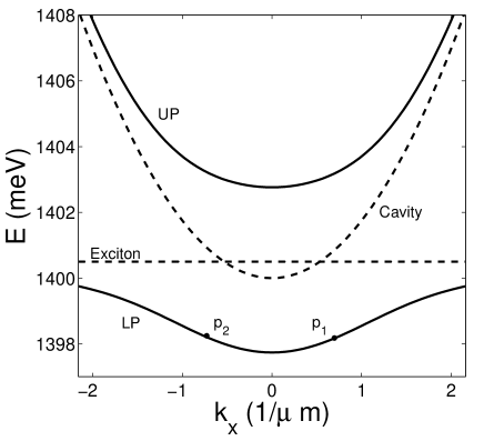
Figure 1: Solid lines: energy dispersion of the Lower and Upper Polariton branches. Dashed lines: the bare quantum well exciton and cavity photon dispersions. The filled circles indicate the wavevectors of the two pumps ($p_{1}$ and $p_{2}$). Note that in the chosen configuration, the photonic fraction of the Lower Polariton at the pump wavevector is $\simeq$ 0.46. Cavity parameters: $\hbar\Omega_{R}=2.5$ meV, $\hbar\omega_{C}^{0}=$ 1400 meV, $\hbar\omega_{X}^{0}=1400.5$ meV, $k_{z}=20\,\mu\textrm{m}^{-1}$. Pump parameters: $k_{p}=0.6981\,\mu\textrm{m}^{-1}$, $\omega_{p}=\omega_{LP}(\mathbf{k}_{p})=1398.2$ meV.

In this work, we will consider the following excitation field:

$$F_{\mathbf{p}}(\mathbf{x},t)=F_{p}\left(e^{-i{k}_{p}{x}}+e^{i{k}_{p}{x}}\right)e^{-i\omega_{p}t}~{}.$$ (9)

This field describes two identical monochromatic plane-wave pumps with opposite wavevectors oriented along the x-axis. Both beams have the same values for the amplitude $F_{p}$ and the frequency $\omega_{p}$. This latter is chosen to be resonant with the LP-branch, i.e. $\omega_{p}=\omega_{LP}(\mathbf{k}_{p})$. Fig. 1 depicts the dispersion of the polariton branches and the position of the pump wavevectors. The scattering process between a pair of $\pm\mathbf{k}_{p}$ pump polaritons via the non-linear interactions, gives rise to a pair of signal/idler polaritons of opposite wavevectors $\pm\mathbf{k}$. Modulo the weak blue-shift of the modes due to interactions, the energy-momentum conservation (phase-matching) is trivially fulfilled if $\omega_{s}=\omega_{i}=\omega_{p}$ and $|\mathbf{k}|={k}_{p}$, that is on the $|\mathbf{k}|={k}_{p}$ parametric luminescence ring.

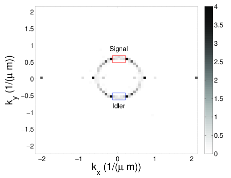
Figure 2: QMC results for the in-cavity photon population $n_{\mathbf{k}}$. Pump amplitude $F_{p}/\gamma=5\,\mu\textrm{m}^{-1}$ (just below the parametric instability threshold). Number of Monte Carlo configurations : 330. The two rectangles denote the areas where the signal and idler are integrated. Cavity parameters: $\hbar\Omega_{R}=2.5$ meV, $\hbar\omega_{C}^{0}=$ 1400 meV, $\hbar\omega_{X}=1400.5$ meV, $k_{z}=$20 $\mu$m^-1, $\hbar\Omega_{R}=2.5$ meV, $\hbar\gamma_{C,X}=\hbar\gamma=0.1$ meV, $\hbar\,g=$ 1.10^-2 meV.$\mu$m^-2. Pump parameters: $k_{p}=$ 0.6981 $\mu$m^-1, $\omega_{p}=\omega_{LP}(\mathbf{k_{p}})=1398.2$ meV. Integration box size $L_{x}=L_{y}=90$ $\mu$m with $n_{x}=n_{y}=64$ points; integration time step $dt=1.7$ fs. Using such a short time step has been necessary in order to obtain sufficient numerical precision on fourth-order field correlation functions.

Fig. 2 shows the numerical results for the stationary state photon population inside the cavity for a value of the pump power below the parametric oscillation threshold: the ring-shaped parametric luminescence pattern is apparent. The interaction-induced blue shift of the polariton modes is responsible for the ring radius being slightly smaller than $k_{p}$. Other interesting features can be observed in addition to the main ring: the strong spots at $\mathbf{k}=\pm 3\mathbf{k}_{p}$ are due to four-wave mixing processes $(\mathbf{k}_{p},\mathbf{k}_{p})\rightarrow(\pm 3\mathbf{k}_{p},\mp\mathbf{k}_{p})$; because of the stimulated nature of the underlying process, these spots fully inherit the coherence of the pump beams. Some luminescence is also observed along the x-axis in the vicinity of $\mathbf{k}_{p}$. Parametric scattering processes involving polaritons from the same pump beam $(\mathbf{k}_{p},\mathbf{k}_{p})\rightarrow(\mathbf{k}_{p}+\delta\mathbf{k},\mathbf{k}_{p}-\delta\mathbf{k})$ with $|\delta\mathbf{k}|\ll|\mathbf{k}_{p}|$ are responsible for this emission. As the pump beams are not tuned at the so-called magic angle, this emission is much weaker than the one on the ring.

In the following, we will focus our attention on signal-idler pairs with wavevectors on the ring, and close to the y-axis ($k_{x}\simeq 0$). To minimize discretization effects, we will average the signal/idler observables on the rectangular areas $\mathcal{D}_{s,i}$ sketched in Fig. 2, which indeed contain quite a number of pixels. The corresponding photon population operators $\hat{N}_{s,i}$ are defined as:

$$\hat{N}_{s,i}=\sum_{\mathbf{k}\in\mathcal{D}_{s,i}}\hat{a}^{{\dagger}}_{\mathbf{k}}\hat{a}_{\mathbf{k}}=N_{D}\hat{n}_{s,i}~{},$$ (10)

where $N_{\mathcal{D}}$ is the number of modes inside $\mathcal{D}_{s,i}$ and $\hat{n}_{s,i}$ are the average photon population operators. In term of the stochastic field, these latter read:

$$\langle\hat{n}_{s,i}\rangle=\frac{1}{N_{D}}\sum_{\mathbf{k}\in\mathcal{D}_{s,i}}\left(\overline{|\alpha_{\mathbf{k}}|^{2}}-\frac{1}{2}\right)~{}.\\$$ (11)

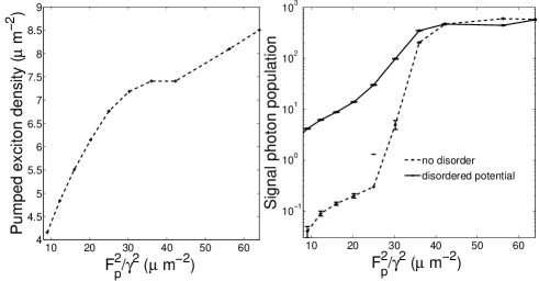
Figure 3: Left panel: QMC results for the density of the pump excitons $\rho_{p}=\langle\hat{b}_{\mathbf{k}_{p}}^{{\dagger}}\hat{b}_{\mathbf{k}_{p}}\rangle/(L_{x}L_{y})$. Right panel: signal/idler photon populations $n_{s,i}$ in the presence (solid line) or absence (dashed line) of the disordered potential. Same cavity and integration parameters as in Fig.2.

The density of pump excitons $\rho_{p}=\langle\hat{b}_{\pm\mathbf{k}_{p}}^{{\dagger}}\hat{b}_{\pm\mathbf{k}_{p}}\rangle/(L_{x}L_{y})$ and the signal/idler populations $n_{s,i}$ are shown as a function of pump power in the left and right panels of Fig. 3 respectively. As previously discussedCarusotto_QMC ; threshold , the pump density $\rho_{p}$ smoothly increases up to the threshold for parametric oscillation. The sub-linear dependence on power stems from the optical limiting effect due to the blue-shift of the $\pm\mathbf{k}_{p}$ modes by the repulsive interactionsIac_Crist_1 . Around the threshold at $F_{p}/\gamma\approx 5.75\,\mu\textrm{m}^{-1}$, $\rho_{p}$ shows a downward kink, while the signal/idler populations have a sudden increase. For the realistic parameters used here, note how the density of excitons at the instability threshold remains moderate, and much lower than the exciton saturation density, $\rho_{\mathbf{k}_{p}}<10^{9}\,{\rm cm}^{-2}\ll\rho_{sat}$. This shows the efficiency of the considered parametric process.

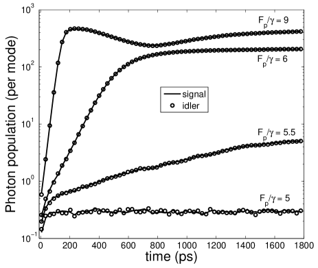
Figure 4: QMC results for $\langle\hat{n}_{s}\rangle$ (Solid line) and $\langle\hat{n}_{i}\rangle$ (circles) as a function of time (ps) for various pump amplitudes across the parametric oscillation threshold: $F_{p}/\gamma=5\,\mu\textrm{m}^{-1}$ (330 configurations), $F_{p}/\gamma=5.5\,\mu\textrm{m}^{-1}$ (340 configurations), $F_{p}/\gamma=6\,\mu\textrm{m}^{-1}$ (180 configurations) and $F_{p}/\gamma=9\,\mu\textrm{m}^{-1}$ (60 configurations). Same cavity and integration parameters as in Fig.2.

In Fig. 4, we can see the temporal spontaneous build-up of the signal and idler luminescence starting from the vacuum fluctuations. For $F_{p}/\gamma=5\,\mu\textrm{m}^{-1}$, the population of the signal/idler modes is still small $n_{s,i}\ll 1$, while stimulated parametric scattering starts to be effective for $F_{p}/\gamma=5.5\,\mu\textrm{m}^{-1}$ when the occupation number is comparable or larger than $1$. The parametric oscillation threshold has already been crossed for $F_{p}/\gamma=6\,\mu\textrm{m}^{-1}$. While the emission ring below threshold has the almost homogeneous intensity profile shown in Fig. 2, a symmetry breaking takes place above the threshold: a few modes are selected by mode competition effects, and a macroscopic population concentrates into them, as shown in Fig.5. It is interesting to note that that the number of Monte Carlo configurations needed for obtaining a given precision in the configuration average strongly depends on the regime under examination: as expected, much less simulations are required above the threshold.

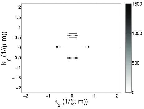
Figure 5: QMC results for the in-cavity photon population $n_{\mathbf{k}}$ for a pump amplitude above the parametric oscillation threshold $F_{p}/\gamma=6\,\mu\textrm{m}^{-1}$. Number of Monte Carlo configurations : 180. Same cavity and integration parameters as in Fig.2.

II.2 In the presence of static disorder

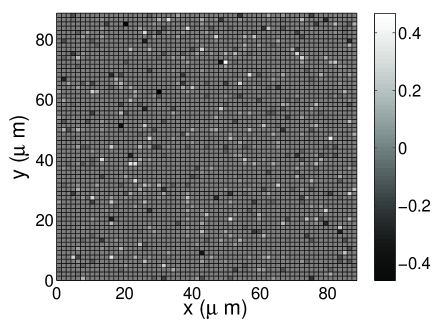
Figure 6: Disordered photonic potential (in meV/$\hbar$) used for the simulations of Fig. 3,7, and 10.

The results in Fig. 2, 4 and 5 have been obtained in the absence of static disorder, i.e. for $V_{C}=V_{X}=0$. An arbitrary potential can be easily included in our calculations. As a specific example, we have considered the disordered photonic potential reported in Fig. 6, consisting of a random ensemble of photonic point defects note . The corresponding emission pattern is shown in Fig. 7 for the same pump parameters as in the clean system of Fig. 2. The main effect of the disorder appears to be a significantly enhanced intensity on the luminescence ring. This occurs because of the resonant Rayleigh scattering of each of the pumps. Note also the weak “eight”-shaped patternCristiano_semi due to the parametric amplification of the resonant Rayleigh scattering ring.

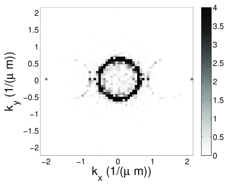
Figure 7: QMC result for the in-cavity photon population $n_{\mathbf{k}}$ in the presence of the disordered potential shown in Fig. 6. The image saturates the gray scale. Pump amplitude $F_{p}/\gamma=5\,\mu\textrm{m}^{-1}$. Number of Monte Carlo configurations : 50. Same cavity and integration parameters as in Fig.2.

The signal population as a function of the pump power is plotted in the right panel of Fig. 3: below threshold, the photon population in the presence of disorder is much larger than in the clean system. On the other hand, the difference between the two populations is much less important above threshold when the non-linear stimulated parametric scattering dominates over the linear Rayleigh scattering processes. Despite the very different low intensity behaviour, the threshold is reached in both cases at values close to $F_{p}/\gamma\simeq 5.5\,\mu\textrm{m}^{-1}$.

III Quantum Correlations

In the present section we study the correlation properties of the signal and idler emissions. For the sake of simplicity, we restrict our attention here to those fluctuations which are associated to the intrinsic losses of the parametrically emitting system, and we neglect all other possible noise sources that may appear in actual experimental setups, e.g. pump intensity fluctuations. To characterize the quantum nature of the correlationsMandel between the signal and idler modes, it is useful to consider the quantity $\hat{N}_{\pm}=\hat{N}_{s}\pm\hat{N}_{i}$ i.e. the sum and difference of the signal and idler photon population. The corresponding normalized noise $\sigma^{\pm}$ reads:

$${\sigma^{\pm}}=\frac{\langle\hat{N}_{\pm}^{2}\rangle-\langle\hat{N}_{\pm}\rangle^{2}}{\langle\hat{N}_{+}\rangle}=\frac{\langle\hat{N}_{s}^{2}\rangle-\langle\hat{N}_{s}\rangle^{2}+\langle\hat{N}_{i}^{2}\rangle-\langle\hat{N}_{i}\rangle^{2}\pm 2\left(\langle\hat{N}_{i}\hat{N}_{s}\rangle-\langle\hat{N}_{s}\rangle\langle\hat{N}_{i}\rangle\right)}{\langle\hat{N}_{i}\rangle+\langle\hat{N}_{s}\rangle}~{}.$$ (12)

Hence, the fourth-order moments of the fields $\langle\hat{N}_{j}\hat{N}_{k}\rangle=\sum_{\mathbf{k}\in\mathcal{D}_{j},\mathbf{k^{\prime}}\in\mathcal{D}_{k}}\langle\hat{n}_{\mathbf{k}}\hat{n}_{\mathbf{k^{\prime}}}\rangle$ (where $j,k\in\{s,i\}$) play a key-role in the determination of the quantum behaviour of the system. In terms of the averaged stochastic quantities we have:

$$\langle\hat{N}_{j}^{2}\rangle = \frac{1}{6}\sum_{\mathbf{k}\in\mathcal{D}_{j}}\left\langle\hat{a}_{\mathbf{k}}^{{\dagger}}\hat{a}_{\mathbf{k}}^{{\dagger}}\hat{a}_{\mathbf{k}}\hat{a}_{\mathbf{k}}+\hat{a}_{\mathbf{k}}^{{\dagger}}\hat{a}_{\mathbf{k}}\hat{a}_{\mathbf{k}}^{{\dagger}}\hat{a}_{\mathbf{k}}+\hat{a}_{\mathbf{k}}^{{\dagger}}\hat{a}_{\mathbf{k}}\hat{a}_{\mathbf{k}}\hat{a}_{\mathbf{k}}^{{\dagger}}+\hat{a}_{\mathbf{k}}\hat{a}_{\mathbf{k}}^{{\dagger}}\hat{a}_{\mathbf{k}}^{{\dagger}}\hat{a}_{\mathbf{k}}+\hat{a}_{\mathbf{k}}\hat{a}_{\mathbf{k}}^{{\dagger}}\hat{a}_{\mathbf{k}}\hat{a}_{\mathbf{k}}^{{\dagger}}+\hat{a}_{\mathbf{k}}\hat{a}_{\mathbf{k}}\hat{a}_{\mathbf{k}}^{{\dagger}}\hat{a}_{\mathbf{k}}^{{\dagger}}\right\rangle-\frac{1}{2}\langle\hat{a}_{\mathbf{k}}^{{\dagger}}\hat{a}_{\mathbf{k}}+\hat{a}_{\mathbf{k}}\hat{a}_{\mathbf{k}}^{{\dagger}}\rangle$$ (13)

$$\phantom{\frac{1}{6}\sum_{\mathbf{k}\in\mathcal{D}_{j}}}+\sum_{\mathbf{k},\mathbf{k^{\prime}}\in\mathcal{D}_{j}}\langle\hat{n}_{\mathbf{k}}\rangle\langle\hat{n}_{\mathbf{k^{\prime}}}\rangle-\sum_{\mathbf{k}\in\mathcal{D}_{j}}\langle\hat{n}_{\mathbf{k}}\rangle\langle\hat{n}_{\mathbf{k}}\rangle$$

$$= \sum_{\mathbf{k}\in\mathcal{D}_{j}}\left(\overline{|\alpha_{\mathbf{k}}|^{4}}-\overline{|\alpha_{\mathbf{k}}|^{2}}\right)+\left(\sum_{\mathbf{k}\in\mathcal{D}_{j}}\left(\overline{|\alpha_{\mathbf{k}}|^{2}}-\frac{1}{2}\right)\right)^{2}-\sum_{\mathbf{k}\in\mathcal{D}_{j}}\left(\overline{|\alpha_{\mathbf{k}}|^{2}}-\frac{1}{2}\right)^{2}~{},$$

with $j=(i,s)$. The intensity correlation between signal and idler modes is:

$$\langle\hat{N}_{s}\hat{N}_{i}\rangle = \frac{1}{4}\sum_{\stackrel{{\scriptstyle\scriptstyle\mathbf{k}\in\mathcal{D}_{s}}}{{\scriptstyle\mathbf{k}^{\prime}\in\mathcal{D}_{i}}}}\left\langle(\hat{a}_{\mathbf{k}}^{{\dagger}}\hat{a}_{\mathbf{k}}+\hat{a}_{\mathbf{k}}\hat{a}_{\mathbf{k}}^{{\dagger}}-1)\right.\left.(\hat{a}_{\mathbf{k^{\prime}}}^{{\dagger}}\hat{a}_{\mathbf{k^{\prime}}}+\hat{a}_{\mathbf{k^{\prime}}}\hat{a}_{\mathbf{k^{\prime}}}^{{\dagger}}-1)\right\rangle$$

$$= \sum_{\mathbf{k}\in\mathcal{D}_{s}}\sum_{\mathbf{k}^{\prime}\in\mathcal{D}_{i}}\overline{|\alpha_{\mathbf{k}}|^{2}\,|\alpha_{\mathbf{k}^{\prime}}|^{2}}-\frac{N_{D}}{2}\left(\sum_{\mathbf{k}\in\mathcal{D}_{s}}\overline{|\alpha_{\mathbf{k}}|^{2}}+\sum_{\mathbf{k}^{\prime}\in\mathcal{D}_{i}}\overline{|\alpha_{\mathbf{k}^{\prime}}|^{2}}-\frac{N_{D}}{2}\right)~{}.$$

For uncorrelated and shot-noise limited signal and idler beams, one would have $\sigma^{\pm}=1$: this value is the so-called Standard Noise LimitWalls . Having $\sigma^{-}<1$ means that non-classical correlations exist between signal and idler, in particular a squeezing of the difference intensity noiseFabre_Treps ; Fabre_Houches . As the polariton states are half-photon half-exciton, the optimal noise reduction of the photon field is reduced by half with respect to an ideal $\chi^{(2)}$ purely photonic parametric oscillator systemLaurat03 ; noise reduction does not concern in fact the photon field taken independently, but rather the whole polariton field. As long as we neglect multiple scattering and disorder effects, this is the main difference compared to standard $\chi^{(2)}$ parametric oscillators; an analytical model for these issues will be provided in Sec.IV. Note that throughout all the present paper we are interested in one-time correlations: the difference noise is therefore integrated over all the frequencies and no frequency filtering is considered. Some frequency filtering around $\omega=\omega_{p}$ would purify the squeezing as the quantum correlations are largest around this value of the frequencyFabre_Cargese .

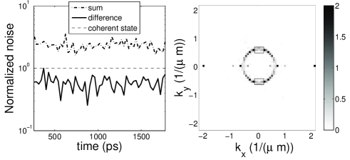
Figure 8: Left panel: QMC results for the time-evolution of the normalized photonic sum and difference noises $\sigma^{\pm}$ in the absence of disorder. Right panel: in-cavity photon population $n_{\mathbf{k}}$ at $t=1800$ ps. Pump amplitude $F_{p}/\gamma=5\,\mu\textrm{m}^{-1}$. Number of Monte Carlo configurations: 330. Same cavity and integration parameters as in Fig.2.

In Fig. 8 we have plotted the time dependance of the normalized noises $\sigma^{\pm}$ for a given Monte Carlo realization and in the absence of disorder. The stationary-state average values for the same quantities are plotted in Fig. 9 as a function of the pump intensity. Quantum correlations $\sigma^{-}<1$ exist in the difference noise at low intensities, while it monotonically increases towards $\sigma^{-}=1$ for higher intensities, making the signal/idler correlations almost purely classical well above thresholdFabre_Treps . No specific feature is found in this quantity at the threshold.

On the other hand, the sum noise $\sigma^{+}$ is always above the standard noise limit, and shows a sudden increase at the parametric threshold. The fact that well above the threshold it does not go back to the standard noise is due to the presence of several competing parametric oscillation modes. Depending on whether the oscillating modes lay inside or outside the selected regions ${\mathcal{D}}_{s,i}$, the signal/idler populations $n_{s,i}$ vary between $0$ and their maximum value, while remaining almost equal to each other. This implies that the sum noise $\sigma^{+}$ is large, of the order of the signal/idler populations $n_{s,i}$ while the difference noise $\sigma^{-}$ remains small.

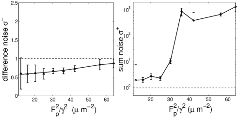
Figure 9: QMC results for the normalized photonic sum and difference noises $\sigma^{\pm}$ as a function of the pump power in the absence of disorder. The difference noise is fitted by a polynomial curve, while the line in the plot for $\sigma^{+}$ is a guide for the eye. Same cavity and integration parameters as in Fig.2.

In Fig.10, we have analyzed the sum and difference noise in the presence of a disordered potential. For the same value of pump intensity, the difference noise $\sigma^{-}$ is now somehow larger than in the absence of disorder: the resonant Rayleigh scattering creates in fact unpaired photons into the luminescence ring and deteriorates the pair correlations between the signal and the idler. For very low intensities, the dominant contribution comes from the Rayleigh scattering processes implying that both the sum and the difference noises have to tend toward the Standard Noise Limit $\sigma^{\pm}=1$. Because of the competition between the Rayleigh and the parametric scattering, the difference noise $\sigma^{-}$ attains its minimum in the vicinity of the threshold and then increases because of the increasing noise of the two beams. As disorder is able to mix the modes respectively inside and outside the selected regions ${\mathcal{D}}_{s,i}$, the difference noise can grow above $\sigma^{-}=1$ at high pump powers. For the same reason, the sum noise $\sigma^{+}$ has a weaker growth above the threshold than in the absence of disorder. This physical interpretation of the role of the disorder has been confirmed by several other simulations (not shown) performed with different realizations of the disordered potential.

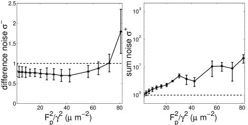
Figure 10: QMC results for $\sigma^{\mp}$ as a function of the pump intensity in the presence of disorder. The lines are a guide for the eye. Same cavity and integration parameters as in Fig.2.

IV Simplified analytical model

The aim of this section is to compare the results of the complete Quantum Monte-Carlo calculations to a simplified input-output analytical model based on a linearization of the Hamiltonian. This is done by treating the intense pump as a classical, undepleted, field, i.e. replacing the pump mode operators with their mean-field expectation values. Obviously, this approximation is valid only well below the parametric oscillation threshold. Concentrating our attention on those processes which satisfy the phase-matching condition and neglecting all the non-resonant others, we can write the linearized Hamiltonian in the following, simplified form:

$$\mathcal{H}=\sum_{\mathbf{k}\neq\mathbf{k}_{p}}\left[\hbar\omega_{C}(\mathbf{k})\hat{a}_{\mathbf{k}}^{{\dagger}}\hat{a}_{\mathbf{k}}+\hbar{\tilde{\omega}_{X}}\hat{b}_{\mathbf{k}}^{{\dagger}}\hat{b}_{\mathbf{k}}\right.\\ +\hbar\Omega_{R}\left(\hat{b}_{\mathbf{k}}^{{\dagger}}\hat{a}_{\mathbf{k}}+\hat{a}_{\mathbf{k}}^{{\dagger}}\hat{b}_{\mathbf{k}}\right)\\ \left.+\hbar\left(\hat{b}_{\mathbf{k}}^{{\dagger}}\hat{b}_{-\mathbf{k}}^{{\dagger}}\kappa+\hat{b}_{\mathbf{k}}\hat{b}_{-\mathbf{k}}\kappa^{*}\right)\right]~{},$$ (15)

where $\hat{b}_{\mathbf{k}}$ is the exciton creation operator, ${\tilde{\omega}_{X}}=\omega_{X}^{0}+\frac{2g}{L_{x}L_{y}}(|\mathcal{P}_{1}|^{2}+|\mathcal{P}_{2}|^{2})$ is the blue-shifted exciton frequency because of interactions, and $\kappa=\frac{g}{L_{x}L_{y}}\mathcal{P}_{1}\mathcal{P}_{2}$ is the effective parametric interaction constant in terms of the pump fields $\mathcal{P}_{1,2}e^{-i\omega_{p}t}=\langle\hat{b}_{\pm\mathbf{k}_{p}}(t)\rangle$. Taking the standard vacuum as the initial state of the photon and exciton fields, the expectation values of the quantum Langevin forces are:

$$\langle\tilde{F}_{cav,\mathbf{k}}[\omega]\tilde{F}^{{\dagger}}_{cav,\mathbf{k}^{\prime}}[\omega]\rangle = 4\pi\Gamma_{cav}[\omega]\delta(\omega-\omega^{\prime})\delta_{\mathbf{k},\mathbf{k}^{\prime}}~{},\$$ (16)

$$\langle\tilde{F}_{exc,\mathbf{k}}[\omega]\tilde{F}^{{\dagger}}_{exc,\mathbf{k}^{\prime}}[\omega]\rangle = 4\pi\Gamma_{exc}[\omega]\delta(\omega-\omega^{\prime})\delta_{\mathbf{k},\mathbf{k}^{\prime}}~{},\$$ (17)

where $\Gamma_{j}[\omega]$ is the complex broadening due to the coupling to the external bath. Since the relevant spectral domain in the degenerate parametric process is concentrated around $\omega_{p}$, we are allowed to simplify the treatment by taking frequency independent linewidth $\Gamma_{ph,exc}[\omega]=\gamma_{C,X}/2$. The quantum Langevin equations in frequency space read:

$$\mathcal{M}_{\mathbf{k},\omega,\omega_{p}}\left(\begin{array}[]{c}\tilde{a}_{\mathbf{k}}[\omega]\\ \tilde{b}_{\mathbf{k}}[\omega]\\ \tilde{a}^{{\dagger}}_{-\mathbf{k}}[2\omega_{p}-\omega]\\ \tilde{b}^{{\dagger}}_{-\mathbf{k}}[2\omega_{p}-\omega]\end{array}\right)=-i\left(\begin{array}[]{c}\tilde{F}_{cav,\mathbf{k}}[\omega]\\ \tilde{F}_{exc,\mathbf{k}}[\omega]\\ \tilde{F}_{cav,-\mathbf{k}}^{{\dagger}}[2\omega_{p}-\omega]\\ \tilde{F}_{exc,-\mathbf{k}}^{{\dagger}}[2\omega_{p}-\omega]\end{array}\right)\begin{array}[]{c}\\ \\ \\ \\ ~{},\end{array}$$ (31)

with the matrix $\mathcal{M}_{\mathbf{k},\omega,\omega_{p}}$ defined for $i=X,C$ as:

$$\mathcal{M}_{\mathbf{k},\omega,\omega_{p}}=\left(\begin{array}[]{cccc}\Delta_{C}(\omega)-i\gamma_{C}/2&\Omega_{R}&0&0\\ \Omega_{R}&\Delta_{X}(\omega)-i\gamma_{X}/2&0&\kappa\\ 0&0&-\Delta_{C}(\omega-2\omega_{p})-i\gamma_{C}/2&-\Omega_{R}\\ 0&-\kappa^{*}&-\Omega_{R}&-\Delta_{X}(\omega-2\omega_{p})-i\gamma_{X}/2\end{array}\right)~{},$$ (36)

in terms of $\Delta_{i}(\omega)=\omega_{i}-\omega$ .

The relation between the time dependent and frequency dependent operators is:

$$\hat{a}_{\mathbf{k}}(t)=\int\frac{d\omega}{2\pi}\tilde{a}_{\mathbf{k}}[\omega]e^{i\omega t},$$ (37)

where $\tilde{a}_{\mathbf{k}}[\omega]$ is the component at $\omega$ of the photonic destruction operator for the $\mathbf{k}$-mode. In the following, we will call $\mathcal{G}_{\mathbf{k},\omega,\omega_{p}}=-i\mathcal{M}_{\mathbf{k},\omega,\omega_{p}}^{-1}$. The signal photon population operator $\hat{n}_{s}(t)$ inside the cavity can be written as:

$$\hat{N}_{s}(t)=\sum_{\mathbf{k}\in\mathcal{D}_{s}}\iint\frac{d\omega}{2\pi}\frac{d\omega^{\prime}}{2\pi}\tilde{a}_{\mathbf{k}}^{{\dagger}}[\omega]\,\tilde{a}_{\mathbf{k}}[\omega^{\prime}]\,e^{-i(\omega-\omega^{\prime})t}~{},$$ (38)

which leads to:

$$\langle N_{s}\rangle=\sum_{\mathbf{k}\in\mathcal{D}_{s}}\int\frac{d\omega}{2\pi}\left(\gamma_{C}|\mathcal{G}_{13}|^{2}[\omega]+\gamma_{X}|\mathcal{G}_{14}|^{2}[\omega]\right).$$ (39)

To calculate the sum and difference noise, the second order momenta $\langle\hat{N}_{s}^{2}\rangle-\langle\hat{N}_{s}\rangle^{2}$, $\langle\hat{N}_{i}^{2}\rangle-\langle\hat{N}_{i}\rangle^{2}$ and $\langle\hat{N}_{i}\hat{N}_{s}\rangle+\langle\hat{N}_{s}\hat{N}_{i}\rangle-2\langle\hat{N}_{i}\rangle\langle\hat{N}_{s}\rangle$ are needed. After some algebra, we obtain the final expressions (for $j=(s,i)$):

$$\langle\hat{N}_{j}^{2}\rangle-\langle\hat{N}_{j}\rangle^{2} = \sum_{\mathbf{k}\in\mathcal{D}_{j}}\int\frac{d\omega}{2\pi}(\gamma_{C}|\mathcal{G}_{13}|^{2}+\gamma_{X}|\mathcal{G}_{14}|^{2})[\omega]\int\frac{d\omega^{\prime}}{2\pi}(\gamma_{C}|\mathcal{G}_{11}|^{2}+\gamma_{X}|\mathcal{G}_{12}|^{2})[\omega^{\prime}]$$ (40)

$$\langle\hat{N}_{s}\hat{N}_{i}\rangle-\langle\hat{N}_{i}\rangle\langle\hat{N}_{s}\rangle = \iint\frac{d\omega_{1}d\omega_{2}}{(2\pi)^{2}}\sum_{k\in\mathcal{D}_{s}}\left(\gamma_{C}\mathcal{G}_{11}^{*}[\mathbf{k},2\omega_{p}-\omega_{1}]\mathcal{G}_{13}^{*}[-\mathbf{k},\omega_{1}]+\gamma_{X}\mathcal{G}_{12}^{*}[\mathbf{k},2\omega_{p}-\omega_{1}]\mathcal{G}_{14}^{*}[-\mathbf{k},\omega_{1}]\right)$$ (41)

$$\left(\gamma_{C}\mathcal{G}_{11}[\mathbf{k},2\omega_{p}-\omega_{2}]\mathcal{G}_{13}[-\mathbf{k},\omega_{2}]+\gamma_{X}\mathcal{G}_{12}[\mathbf{k},2\omega_{p}-\omega_{2}]\mathcal{G}_{14}[-\mathbf{k},\omega_{2}]\right)~{}.$$

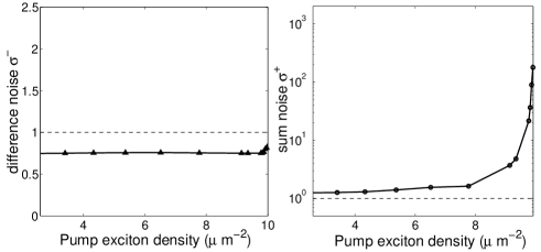
Figure 11: Analytical results for the photonic difference and sum noises $\sigma^{\pm}$ as a function of the pump exciton density $\rho_{p}$ in the absence of disorder. Same cavity and integration parameters as in Fig.2. $\hbar\omega_{p}=\hbar\omega_{LP}(\mathbf{k}_{p})+0.07$ meV $=$ 1398 meV and $\hbar\omega_{X}^{0}=1400.1$ meV.

The results for $\sigma^{-}$ and $\sigma^{+}$ are plotted in Fig. 11. The qualitative similarities between these results and the QMC ones (without disorder) of Fig 9 are apparent for pump intensities up to the parametric threshold. Here, the linearized model breaks down, as it predicts a diverging signal/idler intensity. Although the predictions for the threshold pump intensity differs from the QMC one by approximately twenty percent, still the analytic value in the low intensity limit $\sigma^{-}\simeq 0.75$ is well within the (quite large) error bars of the QMC simulations without disorderfoot_comment . In this limit, the analytical calculation, that neglects interactions between the signal and idler modes, becomes indeed exact and provides a more precise estimation than the QMC calculation. As we have already mentioned, partition noise due to the half photon half exciton nature of the polaritons is responsible for a significantly larger value of $\sigma^{-}$ than in standard $\chi^{(2)}$ parametric emitters Laurat03 . While in the QMC calculations the inclusion of static disorder has been done straightforwardly, the simplified analytical model can not be extended easily to the disorder case, and, most of all, it would lose all its simplicity.

V Conclusion

In conclusion, we have presented a quantum Monte Carlo study of the quantum correlations in the ring-shaped parametric luminescence from semiconductor microcavities in the strong exciton-photon coupling regime. Our results suggest that even in presence of multiple scattering, realistic losses and static disorder, the signal and idler beams maintain a significant amount of quantum correlations. The dependance of the intensity quantum correlation on the pump intensity has been characterized across the parametric instability threshold, showing the regime where the non-classical features are maximized.

We thank G. Bastard, J. Bloch, A. Bramati, C. Diederichs, E. Giacobino, J-Ph. Karr, C. Leyder, N. Regnault, M. Romanelli, Ph. Roussignol and J. Tignon for discussions.

References

- (1) J. Baumberg and L. Viña (Eds.) Special issue on Microcavities, [Semicond. Sci. Technol. 18, S279 (2003)].
- (2) B. Deveaud (Ed.), Special issue on the ”Physics of semiconductors microcavities”, Phys. Stat. Sol. B 242, 2145-2356 (2005) and references therein.
- (3) J. J. Baumberg, P. G. Savvidis, R. M. Stevenson, A. I. Tartakovskii, M. S. Skolnick, D. M. Whittaker and J. S. Roberts, Phys. Rev. B 62, R16247 (2000)
- (4) C. Diederichs, J. Tignon, G. Dasbach, C. Ciuti, A. Lemaître, J. Bloch, Ph. Roussignol and C. Delalande, Nature 440, 904 (2006).
- (5) P. G. Savvidis, J. J. Baumberg, R. M. Stevenson, M. S. Skolnick, D. M. Whittaker and J. S. Roberts, Phys. Rev. Lett. 84, 1547 (2000).
- (6) G. Dasbach, M. Schwab, M. Bayer, D.N. Krizhanovskii and A. Forchel, Phys. Rev. B 66, 201201(R) (2002).
- (7) G. Dasbach, A. A. Dremin, M. Bayer, V. D. Kulakovskii, N. A. Gippius and A. Forchel, Phys. Rev. B 65, 245316 (2002).
- (8) I. Carusotto and C. Ciuti, Phys. Rev. Lett. 93, 166401 (2004).
- (9) J. Ph. Karr, A. Baas, R. Houdré and E. Giacobino, Phys. Rev. A 69, 031802(R) (2004).
- (10) J. Ph. Karr, A. Baas and E. Giacobino, Phys. Rev. A 69, 063807 (2004).
- (11) C. Ciuti, Phys. Rev. B 69, 245304 (2004).
- (12) S. Savasta, O. Di Stefano, V. Savona and W. Langbein, Phys. Rev. Lett. 94, 246401 (2005).
- (13) I. Carusotto and C. Ciuti, Phys. Rev. B 72, 125335 (2005)
- (14) A. Baas, J.-Ph. Karr, M. Romanelli, A. Bramati and E. Giacobino, Phys. Rev. Lett. 96, 176401 (2006).
- (15) P. G. Savvidis, C. Ciuti, J. J. Baumberg, D. M. Whittaker, M. S. Skolnick and J. S. Roberts, Phys. Rev. B 64 075311 (2001).
- (16) M. Romanelli , C. Leyder, J-Ph. Karr, E. Giacobino and A. Bramati, Phys. Rev. Lett. 98, 106401 (2007).
- (17) C. Diederichs, C. Leyder, A. Bramati, D. Taj, T. Lecomte, A. Lemaître, L. Largeau, J. Bloch, C. Ciuti, Ph. Roussignol, C. Delalande, E. Giacobino, J. Tignon, unpublished.
- (18) See, e.g., H. Stolz, D. Schwarze, W. von der Osten, G. Weimann, Phys. Rev. B 47, 9669 (1993); R. Houdré, C. Weisbuch, R. P. Stanley, U. Oesterle, M. Ilegems, Phys. Rev. B 61, R13333 (2000); W. Langbein and J. M. Hvam, Phys. Rev. Lett. 88, 047401 (2002).
- (19) C. Ciuti, P. Schwendimann and A. Quattropani, Semicond. Sci. Technol. 18, S279 (2003).
- (20) A. Kavokin, G. Malpuech and M. Glazov, Phys. Rev. Lett. 95, 136601 (2005).
- (21) I. Shelykh, G. Malpuech, K. V. Kavokin, A. V. Kavokin and P. Bigenwald, Phys. Rev. B 70, 115301 (2004).
- (22) P. G. Lagoudakis, P. G. Savvidis, J. J. Baumberg, D. M. Whittaker, P. R. Eastham, M. S. Skolnick and J. S. Roberts, Phys. Rev. B 65, 161310(R) (2002).
- (23) L. Mandel and E. Wolf, Optical Coherence and Quantum Optics (Cambridge University Press, Cambridge, 1995).
- (24) D.F. Walls and G.J. Milburn, Quantum Optics (Springer-verlag, Berlin, 1994).
- (25) M. Wouters and I. Carusotto, Phys. Rev. B 75, 075332 (2007).
- (26) We have verified that the results do not qualitatively change when different specific potential configurations are used.
- (27) N. Treps and C. Fabre, Laser Phys. 15, 187 (2005), (Preprint quant-ph/0407214).
- (28) C. Fabre, S. Reynaud in Quantum fluctuations, Lecture Notes of Les Houches Summer School Session LXIII, edited by S. Reynaud, E. Giacobino and J. Zinn-Justin. (North-Holland 1995).
- (29) J. Laurat, T. Coudreau, N. Treps, A. Maître, and C. Fabre, Phys. Rev. Lett. 91, 213601 (2003).
- (30) C. Fabre in Confined Photon systems, Fundamentals and Applications, Lectures Notes in Physics of Cargèse Summerschool, edited by H. Benisty, J-M Gérard, R. Houdré, J. Rarity and C. Weisbuch (Springer 1998).
- (31) C. Ciuti and I. Carusotto, Phys. Stat. Sol. B 242, 2224 (2005).
- (32) C. Ciuti, P. Schwendimann, B. Deveaud and A. Quattropani, Phys. Rev. B 62, R4825 (2000).
- (33) M. Saba, C. Ciuti, J. Bloch, V. Thierry-Mieg, R. André, Le Si Dang, S. Kundermann, A. Mura, G. Bongiovanni, J. L. Staehli and B. Deveaud, Nature (London) 414, 731 (2001).
- (34) D. M. Whittaker, Phys. Rev. B 63, 193305 (2001).
- (35) C. Ciuti and I. Carusotto, Phys. Rev. A 74, 033811 (2006).
- (36) A straighforward application of squ eezing theory shows that the exact value is recovered in the limit where the upper polariton can be neglected and the lower polariton is exactly half photon and half exciton.