Propagation of external regulation and asynchronous dynamics
in random Boolean networks

Abstract

Boolean Networks and their dynamics are of great interest as abstract modeling schemes in various disciplines, ranging from biology to computer science. Whereas parallel update schemes have been studied extensively in past years, the level of understanding of asynchronous updates schemes is still very poor. In this paper we study the propagation of external information given by regulatory input variables into a random Boolean network. We compute both analytically and numerically the time evolution and the asymptotic behavior of this propagation of external regulation (PER). In particular, this allows us to identify variables which are completely determined by this external information. All those variables in the network which are not directly fixed by PER form a core which contains in particular all non-trivial feedback loops. We design a message-passing approach allowing to characterize the statistical properties of these cores in dependence of the Boolean network and the external condition. At the end we establish a link between PER dynamics and the full random asynchronous dynamics of a Boolean network.

The main motivation for this work is to study the propagation of external information given by regulating but non-regulated variables into random Boolean networks. This process, called propagation of external regulation, eventually stops due to one of two reasons: Either the external information has propagated throughout the full network, or a core of variables cannot be fixed by PER. The statistical properties of these cores are determined by the ratio $\alpha$ between the numbers of Boolean constraints and of variables, and by the composition of the constraints. In this work we will embed the propagation dynamics of the external condition into the asynchronous update dynamics by introducing ternary variables of values $\{0,1,\star\}$. The supplementary joker value $\star$ indicates that a variable has not been fixed to a Boolean value in the PER dynamics. The introduction of this new value $\star$ allow us to analyze the PER dynamics in terms of a new constraint satisfaction problem with the same topology of the original one, but where Boolean constraints are extended in a natural way in order to include this ternary representation. This observation allows us to apply recently developed tools from the statistical-mechanics approach to combinatorial optimization problems.

I Introduction

Boolean Networks (BNs) are dynamical models originally introduced by S. Kauffman in the late 60s Kauf69 . Since Kauffman’s seminal work, they have been used as abstract modeling schemes in many different fields, including cell differentiation, immune response, evolution, and gene-regulatory networks (for an introductory review see GCK and references therein). In recent days, BNs have received a renewed attention as a powerful scheme of data analysis and modeling of high-throughput genomic and proteomic experiments IlyaBook2005 . Considerable attention has been given in the previous literature to the classification of different attractor types present in BNs under deterministic parallel update dynamics Kauf69 ; Kauf1 ; samuelsson ; BastollaParisi . A special relevance has been attributed to the so-called critical BNs Derrida situated at the transition between an ordered and a chaotic regime.

The original dynamical problem can been cast into a constraint satisfaction problem MPZ ; Libro_Martin . Following this approach presented in letter ; jstat ; fsc-jstat and partially also in Lagomarsino , it is possible to study the organization of fixed points in the thermodynamic limit in random Boolean networks. This leads to the identification of a transition characterized by the sudden emergence of a computational core. Its existence is necessary but not sufficient for a globally complex phase to exist where fixed points are organized in an exponential number of macroscopically separated clusters. This phenomenon is found to be robust with respect to the choice of the Boolean functions. It is missing only in networks where all Boolean functions are of AND or OR type. The size of the complex regulatory phase is found to grow with the number $K$ of inputs of the Boolean functions.

The organization of the paper is the following: in Sec. II we introduce the model focusing to Kauffman models with $K=2$ inputs per Boolean function, in Sec. III we introduce the notion of propagation of external regulation, the message-passing algorithm we will use for analyzing the problem. We also discuss in details the resulting phase diagram of the model. In Sec. IV we will give some analytical prediction on the random asynchronous dynamics of random Boolean networks, and its relation to the PER dynamics. Conclusions are drawn in Sec. V.

II The model

Let us first define properly the model we are going to investigate. It is formed by $N$ Boolean variables collected in a vector $\vec{s}=(s_{1},\dots,s_{N})\in\{0,1\}^{N}$; in Fig. 1 they are represented by circles. They are constrained by Boolean functions $F_{a}(s_{a_{1}},s_{a_{2}})$ with $a\in INT\subset\{1,...,N\}$ running over $M=|INT|$ different variables, each depending on two input variables. The generalization to more than two inputs is obvious, but in this work we will concentrate fully on the two-input case. These functions are represented by squares in Fig. 1 within the so-called factor-graph representation of a BN.

The functions $F_{a}$ allow to define a random asynchronous update dynamics, cf. Gersh ; Drossel : In each step an element $a$ of $INT$ is selected randomly and updated according to its regulating Boolean function

$$s_{a}^{T+1}=F_{a}(s_{a_{1}}^{T},s_{a_{K}}^{T})\ ,$$ (1)

with ${\vec{s}}^{~{}T}$ denoting the configuration after $T$ time steps. This time step is repeated, after $M$ updates every function is selected on average once.

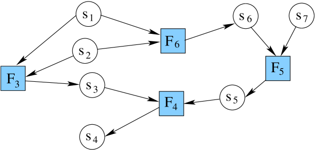
Figure 1: Factor graph representation of a small Boolean network: circles symbolize variables, squares Boolean functions. $s_{1}$ is an example for an external input variable, $s_{4}$ for a functional variable, whereas $s_{3}$ stands for a regulatory variable.

In this work, we concentrate our attention on random factor graphs subject to two conditions:

• Function nodes $F_{a}$ have fixed in-degree $2$ and out-degree one (i.e., two input and one output variable).

• Variables $s_{a}$ have in-degree at most one, i.e., either they depend on one single function, or they are not regulated by any function.

Setting $\alpha:=M/N$, the degree distribution of variable nodes approaches asymptotically

$$\rho^{\mathrm{out}}(d_{\mathrm{out}}) = e^{-K\alpha}\frac{(K\alpha)^{d_{\mathrm{out}}}}{d_{\mathrm{out}}!}$$

$$\rho^{\mathrm{in}}(d_{\mathrm{in}}) = \alpha\delta_{d_{\mathrm{in}},1}+(1-\alpha)\delta_{d_{\mathrm{in}},0}$$ (2)

i.e., the out-degree distribution is a Poissonian of mean $K\alpha$, while in-degree distribution is bimodal. Since in- and out-degrees are uncorrelated, the joint degree distribution factorizes: $\rho(d_{\mathrm{out}},d_{\mathrm{in}})=\rho^{\mathrm{out}}(d_{\mathrm{out}})\rho^{\mathrm{in}}(d_{\mathrm{in}})$. Random factor graphs are obviously a drastic oversimplification of realistic models of gene-regulatory networks: There available data show evidence for a broad, possibly scale-free $\rho^{\rm out}(d_{\rm out})$ and a more concentrated in-degree distribution being compatible with an exponential form GuBoBoKe ; Albert . Nevertheless, this simplified model allows for many detailed analytic predictions that can guide our comprehension in more realistic and interesting cases, and is a well-controlled testing ground for techniques borrowed from statistical mechanics. Such techniques are not limited to random graphs and can be easily extended to deal with more realistic cases.

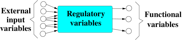
Figure 2: Schematic representation of the three types of variables: external input, functional, and regulatory.

In general, we can distinguish three sets of variables as displayed in Fig. 2:

• External input variables: There are $N-M=(1-\alpha)N$ variables which are not regulated by any function, they are collected in the set $EXT=\{1,..,N\}\setminus INT$. They represent external inputs to the network. We do not consider these external inputs as dynamical variables of the system. In the original definition of Kauffman networks they are in fact included into the definition of the BN itself: This definition works at $\alpha=1$ but allows for constant functions, whose outputs are the analogues of our external input variables.

• Regulatory variables are all those variables which are regulated and regulate.

• Functional variables: There are $e^{-2\alpha}N$ variables which do not regulate any other function.

The last both types form together the set $INT$ of internal, regulated variables. One has to note that in a random network there are some variables which belong theoretically to both the external and the functional variables because they are isolated. They contribute only trivially to the behavior of the network and can therefore be neglected in the discussion.

$s_{1}$	$s_{2}$	0	1	$s_{1}$	$\overline{s_{1}}$	$s_{2}$	$\overline{s_{2}}$	$\wedge$							$\vee$	$\oplus$	$\overline{\oplus}$
0	0	0	1	0	1	0	1	0	0	0	1	1	1	1	0	0	1
0	1	0	1	0	1	1	0	0	0	1	0	1	1	0	1	1	0
1	0	0	1	1	0	0	1	0	1	0	0	1	0	1	1	1	0
1	1	0	1	1	0	1	0	1	0	0	0	0	1	1	1	0	1

Table 1: Truth table for all 16 boolean functions of $K=2$ inputs.

We have to specify the functions acting on top of the random topology defined so far. There are $2^{2^{K}}=16$ Boolean functions, which can be grouped into 4 classes Kauf2 :

• The two constant functions.

• Four functions depending only on one of the two inputs, i.e. $s_{1},\overline{s}_{1},s_{2},\overline{s}_{2}$.

• Canalizing functions (AND-OR class): There are eight functions, which are given by the logical AND or OR of the two input variables, or of their negations. These functions are canalizing. If, e.g., in the case $F(s_{1},s_{2})=s_{1}\wedge s_{2}$ the value of $s_{1}$ is set to zero, the output is fixed to zero independently of the value of $s_{2}$. It is said that $s_{1}$ is a canalizing variable of $F$ with the canalizing value zero.

• Non-canalizing functions (XOR class): The last two functions are the XOR of the two inputs, and its negation. These two functions are not canalizing, whatever input is changed, the output changes too.

We keep in mind that the case of Boolean functions depending on exactly $K=2$ input variables is just the simplest interesting case. Since the number of Boolean functions of $K$ variables increases as $2^{2^{K}}$, a complete classification of Boolean function becomes intractable already for relatively small $K$. For clarity we therefore concentrate first on true $(K=2)$-functions only, i.e. on those in the canalizing AND-OR class and the non-canalizing XOR class. We therefore require $xM$ functions to be in the XOR class, and the remaining $(1-x)M$ functions to be of the AND-OR type, with $0\leq x\leq 1$ being a free model parameter. In this sense, for $K=2$, the network ensemble is completely defined by $\alpha$ and $x$. It is interesting to note that the case $x=1$ on a slightly different class of random hypergraphs, has been already studied in a different context in XOR .

III Propagation of external regulation

An important dynamical process in BN is the propagation of the external condition given by the non-regulated variables into the network. Imagine, e.g., that all inputs of a Boolean function are external variables. Fixing the external condition, also the output of the considered Boolean function is fixed, the external condition has been propagated. Iterating this propagation, we may eventually also fix variables which do not depend directly on external variables, but whose inputs have been fixed in an earlier iteration step, cf. Fig. 3. Note that in the case of canalizing functions it is sufficient to have one input variable fixed to its canalizing value in order to be able to propagate the information. Thus, PER is more efficient in the case of a small fraction $x$ of non-canalizing, XOR-type functions in the network.

This propagation of external regulation may stop in two ways: First, all variables might be fixed, and the external information is propagated throughout the full network. Second, a core of functions survives which still have unfixed output. This PER core contains in particular all relevant feed-back loops which are not broken due to the inclusion of canalizing functions.

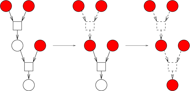
Figure 3: PER: Both inputs to the upper left Boolean function are external, so also the output is directly fixed. Once this is done, also the inputs to the second function are fixed, and again the information can be propagated. All variables in this small sample graph are therefore determined by PER, no core exists.

The propagation dynamics of the external condition can be embedded into the asynchronous update dynamics of Eq. (1) by generalizing the Boolean variables to ternary variables, and the Boolean functions accordingly. In addition to the values 0 and 1 we introduce the joker value $\star$ for variables having no fixed value. As an initial condition for PER, only the external variables have assigned Boolean values, whereas all nodes belonging to $INT$ are assigned value $\star$. Generalizing the functions according to Tab. 2, the dynamics of PER is given exactly by Eq. (1), with a randomly selected $a\in INT$ for each single-variable update.

$s_{1}$	$s_{2}$	$\wedge$							$\vee$	$\oplus$	$\overline{\oplus}$
0	0	0	0	0	1	1	1	1	0	0	1
0	1	0	0	1	0	1	1	0	1	1	0
0	$\star$	0	0	$\star$	$\star$	1	1	$\star$	$\star$	$\star$	$\star$
1	0	0	1	0	0	1	0	1	1	1	0
1	1	1	0	0	0	0	1	1	1	0	1
1	$\star$	$\star$	$\star$	0	0	$\star$	$\star$	1	1	$\star$	$\star$
$\star$	0	0	$\star$	0	$\star$	1	$\star$	1	$\star$	$\star$	$\star$
$\star$	1	$\star$	0	$\star$	0	$\star$	1	$\star$	1	$\star$	$\star$
$\star$	$\star$	$\star$	$\star$	$\star$	$\star$	$\star$	$\star$	$\star$	$\star$	$\star$	$\star$

Table 2: Extended truth table for canalizing and non-canalizing functions of $K=2$ inputs.

Note that, the fraction of variables reached by PER depends not only on the network but also on the precise external condition. In a previous publication jstat , we have analyzed the average case which is realized by the vast majority of external conditions. Here we are aiming at a more precise description of fluctuations of the PER core size due to various external conditions. Note that such fluctuations are completely due to the existence of canalizing functions which may or may not propagate the information of a single fixed input, in dependence on whether it has its canalizing value or not. For $x=1$ we thus expect no such fluctuations to exist, and the PER core is completely topological in the sense that it depends only on the underlying network and not the actual realization of the functions.

III.1 Belief propagation for the ensemble of PER cores

The algorithmic determination of the PER core for a single external condition can be achieved in linear time by simply following the definition of the process itself. If we want to characterize the statistical properties of the ensemble of all cores resulting from $2^{(1-\alpha)N}$ external conditions, running times obviously become exponential and thus not feasible for large networks.

The introduction of the joker value allows us to set up a directed belief-propagation algorithm Yedidia ; SumProd ; BMZ which may be used to efficiently describe the statistical properties of all regulated variables over all external conditions. Some interesting limiting cases will be discussed separately: The appearance of the first PER cores in an exponentially small fractions of all external conditions, the appearance of the PER core for a typical external condition, and the appearance of a non-zero overlap of all PER cores.

As already mentioned, we are interested in the behavior for the full ensemble of external configurations. We therefore introduce the single-site distributions

$$p_{i}(s)=2^{-(1-\alpha)N}\sum_{\rm ext.\ cond.}\delta_{s_{i},s}$$ (3)

as the histogram of the value of variable $s_{i}$ over all external conditions, after completion of PER. In this notation, an external variable obviously has

$$p_{i}(s)=\frac{1}{2}\delta_{s,0}+\frac{1}{2}\delta_{s,1},\ \ \ \ i\in EXT$$ (4)

since by definition it never takes value $\star$, whereas internal variable might have a non-trivial weight also in $p_{i}(\star)$.

Under PER, these probabilities get updated as

$$p_{i}(s_{i})=\sum_{s_{j},s_{k}}\delta_{s_{i},F_{i}(s_{j},s_{k})}\ p_{j}(s_{j})\ p_{k}(s_{k})\ ,$$ (5)

following the output of the extended Boolean function summed over all possible input configurations. In this equation, variable $s_{i}$ is understood to be regulated by $s_{j}$ and $s_{k}$. These equations can be understood as a directed Belief propagation (BP). Note that the BP equations contain a very important assumption: The probability of the two regulating variables is factorized, i.e., they are assumed to be statistically independent. This assumption is expected to become asymptotically exact in the thermodynamic limit $N\to\infty$ of infinitely large random Boolean networks. In finite networks, it might be violated due to short loops: The input variables $s_{i}$ and $s_{j}$ might, e.g., depend on two Boolean functions with a common input and thus be correlated. More generally correlations between two input variables are introduced whenever they have some common ancestor. In random network such ancestors are known to typically have a distance of ${\cal O}(\ln N)$, and thus become irrelevant in the case of very large BNs (inside on thermodynamic state).

The update can be achieved iteratively, starting from the initial condition

$$p_{i}^{0}(s)=\left\{\begin{array}[]{ccl}\frac{1}{2}\delta_{s,0}+\frac{1}{2}\delta_{s,1}&&{\rm for}\ i\in EXT\\ \delta_{s,\star}&&{\rm for}\ i\in INT\\ \end{array}\right.$$ (6)

which reflects the fact that initially only the external variables are fixed, and the regulated ones are still unknown.

Note that the original PER is included in Eq. (5) if the external condition is polarized completely to a single configuration. In this moment, all marginal probabilities remain polarized into one of the three possible values, and factorization in Eq. (5) becomes trivially fulfilled. Under this initial condition, BP would be exact on whatever Boolean network.

Since BP equations are defined on a single graph, their applicability is not necessarily restricted to random BNs with their Poissonian outdegree distribution. In the latter case one can, however, introduce a simple average over the graph ensemble by introducing the histogram of the $p_{i}(\cdot)$ for all internal variables:

$${\cal P}[\,p(\cdot)\,]=\frac{1}{\alpha N}\sum_{i\in INT}\delta[\,p(\cdot)-p_{i}(\cdot)\,]$$ (7)

with $\delta[\cdot]$ being a three-dimensional Dirac distribution in all components of $p_{i}$. For a randomly chosen regulated variable, each of the inputs is regulated with probability $\alpha$, and external else. So we can write an effective self-consistent equation for $P$,

$${\cal P}[\,p(\cdot)\,] = \int{\cal D}p_{1}{\cal D}p_{2}{\cal Q}[\,p_{1}(\cdot),\alpha\,]{\cal Q}[\,p_{2}(\cdot),\alpha\,]$$ (8)

$$\times \left\langle\delta\left[p(\cdot)-\sum_{s_{1},s_{2}}\delta_{\cdot,F(s_{1},s_{2})}\ p_{1}(s_{1})\ p_{2}(s_{2})\right]\right\rangle_{F}\,\,\,\,\,\,\,\,$$

where

$${\cal Q}[\,p(\cdot),\alpha\,]=\alpha{\cal P}[\,p(\cdot)\,]+(1-\alpha)\delta\left[\,p_{1}(\cdot)-\frac{1}{2}(\delta_{\cdot,0}+\delta_{\cdot,1})\,\right]$$ (9)

In this equation, each integration runs over a three-dimensional simplex, and the average $\langle\cdot\rangle_{F}$ is taken over the distribution of Boolean functions at given fraction $x$ of non-canalizing functions. It can be solved iteratively by standard methods as population dynamics, but some limiting cases can be discussed analytically.

III.2 The appearance of the first PER core

For small $\alpha$, only few regulated variables exist in comparison to the number of external variables. As already shown in letter ; jstat , for $\alpha<1/(1+x)$ typically all variables can be fixed by PER starting from the external condition. Typically here means that, starting from a randomly chosen external configuration and with probability approaching one in the thermodynamic limit, no extensive PER core remains.

On the other hand, one should expect that an exponentially small fraction of external conditions already leads to a non-zero PER core at smaller $\alpha$. This happens if external variables are chosen to take as rarely as possible canalizing values of the Boolean functions depending on them.

The argument can be made mathematically more stringent. For doing so, we first observe that the existence of a PER core for some external configurations leads to a finite fraction of variables $i$ with $p_{i}(\star)>0$.

We therefore introduce the fractions of regulated variables never (resp. always) taking a certain value $s$ out of $\{0,\star,1\}$

$$\tau_{s} = {\cal P}[p(s)\equiv 0]\ =\ \frac{1}{\alpha N}\sum_{i\in INT}\delta_{p_{i}(s),0}\ ,$$

$$\pi_{s} = {\cal P}[p(s)\equiv 1]\ =\ \frac{1}{\alpha N}\sum_{i\in INT}\delta_{p_{i}(s),1}\ .$$ (10)

The existence of an extensive core for some of external conditions is obviously equivalent to $\tau_{\star}<1$. Note that in our unbiased ensemble of Boolean functions none of the values zero or one is favored. We thus expect $\tau_{0}=\tau_{1}$ and $\pi_{0}=\pi_{1}$ for symmetry reasons.

III.2.1 Fixed-point equations

We can use the BP equations to get a finite closed set of equations including $\tau_{\star}$. Technically this means to project Eq. (8), which is formulated as an equation for functions over a three-dimensional simplex, to a finite number of variables. To achieve this, we have to discuss carefully all those cases on the right-hand side of Eq. (8) which lead to a vanishing probability for $s=\star$ on the left-hand side.

• For non-canalizing functions, a non-zero probability of a $\star$-valued output exists whenever one of the inputs is allowed to assume also value $\star$. To contribute to $\tau_{\star}$, both inputs have to be non-$\star$, which happens with probability $(1-\alpha+\alpha\tau_{\star})^{2}$.

• For canalizing functions, the situation is a bit more involved. The output is prevented from taking value $\star$ also if one of the inputs is frozen completely to its canalizing value, which (due to the symmetry discussed above) happens with probability $\alpha\pi_{0}=\alpha\pi_{1}$. To avoid double counting with the previously discussed case, the second input than has to have a non-zero probability in $\star$, which happens with $\alpha(1-\tau_{\star})$

Putting the two cases together, we find

$$\tau_{\star} = x(1-\alpha+\alpha\tau_{\star})^{2}+(1-x)[(1-\alpha+\alpha\tau_{\star})^{2}+2\alpha^{2}\pi_{0}(1-\tau_{\star})]$$ (11)

$$= (1-\alpha+\alpha\tau_{\star})^{2}+2(1-x)\alpha^{2}\pi_{0}(1-\tau_{\star})\ .$$

This equation still depends on the probability $\pi_{0}=\pi_{1}$ that a variable is frozen to one of the values 0 or 1. By definition, this can happen only to regulated variables, but even there only if either both inputs are frozen to a fixed value from $\{0,1\}$ or if one input of a canalizing function is frozen to its canalizing value. In this sense, frozen variables are generated only by other frozen variables. On the other hand, the initial condition of Eq. (6) does not contain such frozen values, and under iteration of Eq. (5) they cannot be generated spontaneously. We thus conclude

$$\pi_{0}=\pi_{1}=0\ ,$$ (12)

and Eq. (11) reduces to

$$\tau_{\star}=(1-\alpha+\alpha\tau_{\star})^{2}\ .$$ (13)

This equation does not depend on the fraction $x$ of canalizing functions any more. It has two solutions, a trivial one relevant for small $\alpha$, a non-trivial one for higher $\alpha$. More precisely we find

$$\tau_{\star}=\left\{\begin{array}[]{cl}1&{\rm if}\ \alpha<\frac{1}{2}\\ \frac{(1-\alpha)^{2}}{\alpha^{2}}&{\rm if}\ \alpha>\frac{1}{2}\end{array}\right.$$ (14)

Note that also the solution $\tau_{\star}=1$ is physically sensible beyond $\alpha=1$. The derivation of Eq. (11) requires only consistency of the generalized Boolean functions, which is obviously also fulfilled for any fixed point of the BN containing no $\star$-valued variables. The correct solution for the PER core is given by both the consistency of functions and the maximality of the number of $\star$, which results from the fact that only those internal variables are changed from $\star$ to $0$ or $1$ which are necessary for fulfilling the generalized Boolean constraints. This will become more clear in in next subsection.

The result is quite interesting. Independently of the fraction of canalizing Boolean functions, the PER cores for some external conditions start to exist as soon as $\alpha$ exceeds 1/2. Note that also the fraction of concerned variables does not depend on $x$. According to the above discussion that the PER core for a BN without canalizing functions is uniquely determined and of purely topological nature, the same is true for the set of variables which are contained at least in one PER core. This set does not depend on the choice of functions, but only on the underlying graph structure.

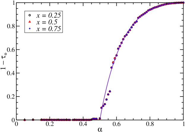
Figure 4: Fraction of internal variables being in at least one PER core: Analytical result (full line) versus BP results on single graphs of $N=10000$ vertices.

In Fig. 4 we compare the analytical result to the BP result on single BNs of $N=10000$ vertices, for various values of $\alpha$. We plot the fraction $1-\tau_{\star}$ of all those internal vertices which belong to the PER core for at least one external configuration. Besides the good coincidence between analytical results (derived in the thermodynamic limit) and single-sample data, one point is remarkable: The BP curves for various $x$-values are practically identical. They come from identical graphs with different realizations of the functions, showing thus that the union of the PER cores for all external conditions is a topological object of the underlying graph.

III.2.2 Dynamics

To close this subsection, we discuss shortly the dynamics of $\tau_{*}(t)$ as a time dependent quantity. Let us assume a random asynchronous update. Then the expected number of sites contributing to $\tau_{\star}$ after $T$ single-variable updates is given by

$$M\tau_{\star}(T+1)=M\tau_{\star}(T)-\tau_{\star}(T)+(1-\alpha+\alpha\tau_{\star}(T))^{2}\ .$$ (15)

On the right-hand side, we have three contributions: the number of contributing sites after step $T$, the probability that the randomly selected internal site already contributes, and the probability that the inputs to this site at step $T$ force the variable to contribute at step $T+1$. Note that we have already canceled the constantly vanishing $\pi_{0}$ contribution in Eq. (11). In the thermodynamic limit we rescale the time as $t=T/M$, and the above equation becomes an ordinary differential equation,

$$\dot{\tau}_{\star} = -\tau_{\star}+(1-\alpha+\alpha\tau_{\star})^{2}$$ (16)

$$= \left(\alpha^{2}\tau_{\star}-[1-\alpha]^{2}\right)\ (\tau_{\star}-1)$$

with the initial condition $\tau_{\star}(t=0)=0$. This equation is solved by

$$\tau_{\star}(t)=\left\{\begin{array}[]{cl}\frac{(1-\alpha)^{2}}{\alpha^{2}}\frac{1-\exp\{(1-2\alpha)t\}}{1-\frac{(1-\alpha)^{2}}{\alpha^{2}}\exp\{(1-2\alpha)t\}}&{\rm if}\ \alpha\neq\frac{1}{2}\\ \frac{t}{t+4}&{\rm if}\ \alpha=\frac{1}{2}\end{array}\right.$$ (17)

which, starting from zero, grows monotonously toward the fixed point given in Eq. 14. Note that the approach to the fixed point is in general exponentially fast, but it slows down algebraically at the critical point, there the asymptotic approach happens as $t^{-1}$. Note also that, due to the initial condition $\tau_{\star}(t=0)=0$ the dynamics stops as soon as it reaches the smallest fixed-point of $\tau_{\star}$, which corresponds to the selection of the largest number of $\star$, and justifies our previous selection of the relevant solution.

III.3 Appearance and size of the typical PER core

III.3.1 Fixed-point equations

In the last subsection, we have seen that the first extensive PER cores appear continuously at $\alpha=1/2$, independently of the value of the fraction $x$ of non-canalizing functions. These cores correspond, however, to an exponentially small fraction of all external conditions. The average core size remains zero in the thermodynamic limit. We can use the self-consistent equation (8) in order to determine the average fraction of regulated nodes in the PER core,

$$n_{PER}=\int{\cal D}p\ {\cal P}[p]\ p(\star)\ .$$ (18)

It can also be interpreted as the typical PER-core size, since a randomly chosen external condition leads to this size with a probability approaching one in the thermodynamic limit $N\to\infty$.

As already derived within a slightly different way in letter ; jstat this size is given by the self-consistent equation

$$1-n_{PER}=(1-\alpha n_{PER})^{2}+(1-x)(1-\alpha n_{PER})\alpha n_{PER}\ .$$ (19)

The first contribution comes from a situation where both parent nodes are not in the core, the second from canalizing functions with one canalizing and one core input. This equation has two solutions, the physically relevant one is the larger one:

$$n_{PER}=\left\{\begin{array}[]{cl}0&{\rm if}\ \alpha\leq\frac{1}{1+x}\\ \frac{\alpha(1+x)-1}{x\alpha^{2}}&{\rm if}\ \alpha>\frac{1}{1+x}\end{array}\right.$$ (20)

This implies that the PER core typically appears only at $\alpha>1/(1+x)$, which goes from $\alpha=1$ at $x=0$ to $\alpha=1/2$ at $x=1$. For purely canalizing networks we thus find that the typical core size remains always zero, even if some rare core exist beyond $\alpha=1/2$, whereas for purely non-canalizing BNs both threshold coincide since the PER core in this case does not depend on the external condition.

III.3.2 Dynamics

The dynamical evolution of this quantity can be derived following the same procedure as in the last subsection. We immediately give the resulting rate equation

$$\dot{n}_{PER}(t)=[\alpha(1+x)-1]\ n_{PER}(t)-\alpha^{2}\,x\,n_{PER}^{2}(t)$$ (21)

Initially all internal variables are $\star$, so we have the initial condition $n_{PER}(0)=1$. This ordinary differential equation is readily solved by

$$n_{PER}(t)=\left\{\begin{array}[]{cl}{\rm max}\left[0,g(t|\alpha,x)\right]&{\rm if}\ \alpha\neq\frac{1}{1+x}\\ \frac{1}{1+\alpha^{2}\,x\,t}&{\rm if}\ \alpha=\frac{1}{1+x}\end{array}\right.$$ (22)

where

$$g(t|\alpha,x)=\frac{(\alpha(1+x)-1)\exp\{[\alpha(1+x)-1]\,t\}}{x\alpha^{2}+[\alpha(1+x)-1-x\alpha^{2}]}$$ (23)

Note that for the subcritical case, the system reaches $n_{PER}=0$ after finite time, whereas it reaches its asymptotic value exponentially fast in the supercritical phase. Exactly at the transition we see the expected algebraic decay.

III.4 The intersection of all PER cores

As a last special case which can be investigated analytically we look at the intersection of the PER cores for all external conditions. The question is: Are there variables never fixed by PER? How many of these variables exist in a network? As before, we will first discuss the fixed point equations for the size of the intersection, and derive the phase-transition line for a non-trivial size. Than we are going to discuss the dynamics of PER, and how the physically relevant solution is selected.

III.4.1 Fixed-point equations

We are interested in the variables which are $\star$ for all external conditions. Their fraction amongst the regulated variables equals $\pi_{\star}$, according to Eq. (III.2). Let us discuss under which input conditions the output of a generalized Boolean function becomes constantly $\star$:

• Non-canalizing functions: The output is fixed to $\star$ if and only if at least one input is regulated and fixed to $\star$. This happens with probability $[1-(1-\alpha\pi_{\star})^{2}]$.

• Canalizing functions: Here the situation is a bit more involved. The output is obviously $\star$ if both inputs are $\star$. If only one input is $\star$, the other one is not allowed to take its canalizing value - i.e. one input is “frozen” to $\star$, the other “frozen away” from its canalizing value. The cumulative probability of all these cases is $[2\alpha^{2}\pi_{\star}\tau_{0}-\alpha^{2}\pi_{\star}^{2}]$. The negative term removes the double-counting of the case of two $\star$-valued inputs. Note that this is strictly true for the AND function having canalizing values equal to zero for both inputs. For the other functions it follows from the symmetry condition $\tau_{0}=\tau_{1}$.

We thus find

$$\pi_{\star}=x\left[1-(1-\alpha\pi_{\star})^{2}\right]+(1-x)\left[2\alpha^{2}\pi_{\star}\tau_{0}-\alpha^{2}\pi_{\star}^{2}\right]$$ (24)

This equation depends still on $\tau_{0}$, i.e., on the probability that a variable is frozen away from $x=0$. We consider the following cases

• Non-canalizing functions: There are two types of contributions: In the first one, at least one input is frozen to $\star$, i.e. the output becomes $\star$ too, and thus differs from zero. The second contribution stems from the situation, where non of the variables is frozen to $\star$, we have to avoid any input configuration producing zero (00 and 11 for XOR, 01 and 10 for its negation). The total probability for this is $[1-(1-\alpha\pi_{\star})^{2}+2\alpha^{2}(\tau_{0}-\pi_{\star})^{2}]$.

• Canalizing functions, canalized output equals zero: None of the inputs is allowed to assume the canalizing value, which has probability $\alpha^{2}\tau_{0}^{2}$.

• Canalizing functions, canalized output equals one: Only the simultaneous appearance of two non-canalizing input variables has to be avoided, the corresponding probability reads $[1-(1-\alpha\tau_{0})^{2}]$.

The total equation for $\tau_{0}$ thus reads

$$\tau_{0}=x\left[1-(1-\alpha\pi_{\star})^{2}+2\alpha^{2}(\tau_{0}-\pi_{\star})^{2}\right]+(1-x)\alpha\tau_{0}\ .$$ (25)

Eqs. (24,25) are two closed quadratic equations, thus they can be solved analytically. The solutions are:

1. The trivial solution

   $$\pi_{\star}=\tau_{0}=0$$ (26)

2. A second solution of trivial $\pi_{\star}$

   $$\pi_{\star}=0,\ \ \ \ \ \tau_{0}=\frac{1+\alpha(x-1)}{2\alpha^{2}x}$$ (27)

3. The potentially physical solution

   $$\pi_{\star} = \frac{1+x-4x^{2}+\alpha(-1-2x+3x^{2}+4x^{3})+(x-1)D}{2\alpha^{2}x(2x^{2}-1)}$$

   $$\tau_{0} = \frac{1-4x^{2}+\alpha(-1-3x+4x^{2}+8x^{3})+D}{4\alpha^{2}x(2x^{2}-1)}$$ (28)

   with

   $$D=\sqrt{1+\alpha(-2-6x+8x^{3})+\alpha^{2}(1+6x+x^{2}-8x^{3})}$$ (29)

4. The unphysical solution

   $$\pi_{\star} = \frac{1+x-4x^{2}+\alpha(-1-2x+3x^{2}+4x^{3})-(x-1)D}{2\alpha^{2}x(2x^{2}-1)}$$

   $$\tau_{0} = \frac{1-4x^{2}+\alpha(-1-3x+4x^{2}+8x^{3})-D}{4\alpha^{2}x(2x^{2}-1)}$$ (30)

The first solution is the correct one for small enough $\alpha$. The third one becomes potentially relevant, when the argument under the square root becomes positive, i.e., when $D$ is a positive real number. This point is actually relevant for small $x$, for larger $x$ the corresponding $\pi_{\star}$ would be negative. It becomes positive only at $\alpha=1/(2x)$ as can be seen easily by linearizing the above equations. To summarize, the non-trivial solution becomes physical beyond the phase transition line

$$\alpha(x)=\left\{\begin{array}[]{cll}\frac{1+3x-4x^{3}+2\sqrt{2x^{2}-6x^{3}+4x^{6}}}{1+6x+x^{2}-8x^{3}}&{\rm for}\ x<\frac{1+\sqrt{17}}{8}&\\ \frac{1}{2x}&{\rm for}\ x\geq\frac{1+\sqrt{17}}{8}&\\ \end{array}\right.$$ (31)

In this equation, we have already indicated the character of the transition: For $x$ below the tricritical point $(1+\sqrt{17})/8\simeq 0.640388$, the transition is discontinuous, and the intersection of all PER cores jumps from an empty set to a non-zero fraction of all internal vertices. Above this point, a non-trivial intersection appears continuously crossing the critical line. In Fig. 5, this analytical result is shown to be well-confirmed by the BP results on a single graph of 10000 vertices.

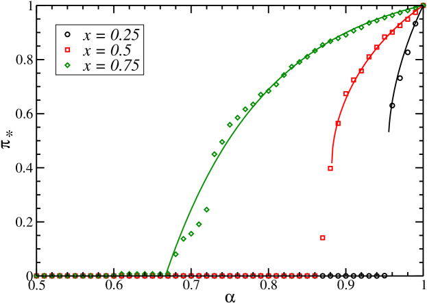
Figure 5: Fraction of internal variables being in all PER cores: Analytical result (full lines) versus BP results (symbols) on single graphs of $N=10000$ vertices.

III.4.2 Dynamics

As before, the selection of the relevant solution can be justified by the dynamical behavior of PER. Following the same arguments as above, we can write down two coupled ordinary differential equations for the evolution of both $\pi_{\star}$ and $\tau_{0}$ which are expected to be exact in the thermodynamic limit of large BNs. The equations are

$$\dot{\pi}_{\star} = -\pi_{\star}+x\left[1-(1-\alpha\pi_{\star})^{2}\right]+$$

$$(1-x)\left[2\alpha^{2}\pi_{\star}\tau_{0}-\alpha^{2}\pi_{\star}^{2}\right]$$

$$\dot{\tau}_{0} = -\tau_{0}+x\left[1-(1-\alpha\pi_{\star})^{2}+2\alpha^{2}(\tau_{0}-\pi_{\star})^{2}\right]+$$ (32)

$$(1-x)\alpha\tau_{0}$$

which have to be solved simultaneously under the initial condition

$$\pi_{\star}(t=0)=\tau_{0}(t=0)=1$$ (33)

corresponding to the fact that initially all internal variables are set constantly to $\star$. Unfortunately, we did not find a closed analytical form for the solution of Eqs. (III.4.2), the results of a numerical integration are represented in Fig. 6. One can beautifully see the difference between the discontinuous transition at low $x$ via the formation of a finite-hight plateau, and the continuous transition at higher fraction $x$ of non-canalizing functions. In Fig. 7 the result of Eqs. (III.4.2) is plotted together with the actual BP dynamics on a single BN of $N=10000$ variables, for $x=0.5$ and various values of $\alpha$ below and above the transition point $\alpha(x)\simeq 0.88185$. Both are completely consistent, as to be expected sample-to-sample fluctuations are large close to the transition, such that the self-averaging properties of $\pi_{\star}$ and $\tau_{0}$ show up clearly only for larger samples.

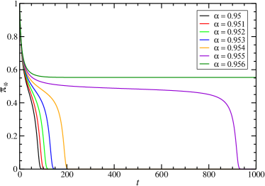
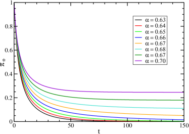
Figure 6: Time dependence of the number of variables frozen to $\star$ under random asynchronous PER, for $x=0.25$ (left figure) and $x=0.75$ (right figure). For small $x$, the discontinuous character of the transition can be beautifully seen from the appearance of a non-zero plateau, whose length diverges at the phase-transition point ($\alpha\simeq 0.95505$ for $x=0.25$). The transition is continuous for large $x$, as can be seen in the right figure.

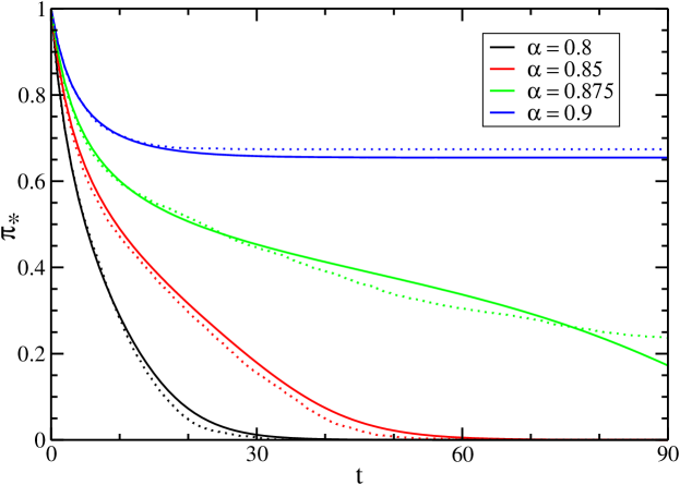
Figure 7: Comparison of the analytical description (full lines) with realizations in single random BNs of $N=10000$ vertices (dotted lines). Up to sample-to-sample fluctuations, the results coincide.

III.5 The phase diagram

The findings are summarized in the phase diagram in Fig. 8. We can distinguish four different regions

• For $\alpha<0.5$ (left of the blue vertical line), all external information propagates throughout the system, with probability one no PER core exists.

• For $\alpha$ between the blue and the black lines, some external conditions lead to a PER core. Almost all conditions, however, propagate throughout the full systems, a random external condition leaves almost surely no core.

• For $\alpha$ in between the black and the red/green curves, a typical external condition leads to an extensive core. The core size starts to grow continuously at the black line, and increases when entering deeper into this phase.

• For $\alpha$ beyond the red/green curve, all PER cores overlap, the intersection of all cores is non-empty. The transition is discontinuous for small $x$ (green line), and continuous for larger $x$ (red line).

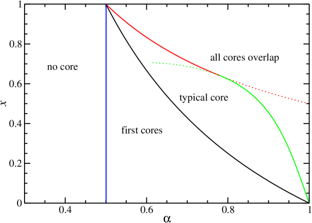
Figure 8: Phase diagram for PER on random Boolean networks. The dotted lines correspond to the unphysical parts of the phase transition lines.

III.6 The distribution of PER-core sizes

It is interesting to see directly what the distribution of the PER cores size look like in single instances of BNs. To do so we have generated graphs at $\alpha=0.95$ for different concentrations of non-canalizing functions $x=(0,0.1,0.4)$ and different sizes $N=100,200,400$. Given a single instance of the BN one can calculate the PER core sizes generated for each of the $2^{(1-\alpha)N}$ configurations of external variables, and finally compute their distribution. Although the time needed for computing a PER core is linear in $N$, we have to explore an exponential of number of external conditions, which constrains us to work at relatively small $N$ and at values of $\alpha$ very close to 1.

In Fig. 9 we display the histogram of the the core size density averaged over 60000 different samples. We also display the theoretical value for the average core size as computed already in jstat (displayed as a black thick arrows). The emerging scenario is coherent with the analytic predictions:

• For $x=0$ we are in the “first cores” phase where each of the external conditions fix almost all the variables as indicated by the concentration of the weight of the histogram around 0 (see left panel in Fig. 9).

• For $x=0.1$ we are in the “typical cores” phase characterized by the formation of the small peak at high values of the core size density. Yet many of the external conditions fix almost all the variables as indicated by the concentration of the weight of the histogram around 0 (see left panel in Fig. 9). In this region finite size scaling corrections are relevant probably due to the nearby phase transition line.

• For $x=0.4$ we are in the “all cores overlapping” phase and the histogram peaks nicely close to the theoretical mean value. The noisy signal at small core sizes is due to strong sample to sample fluctuations.

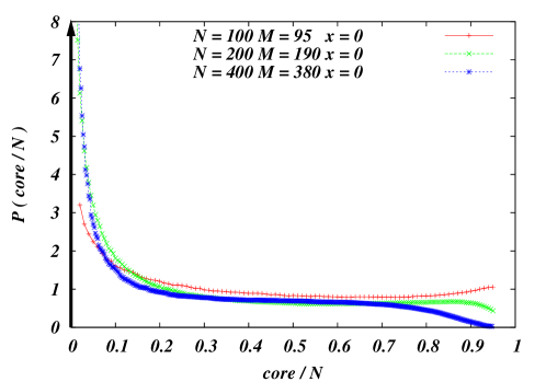
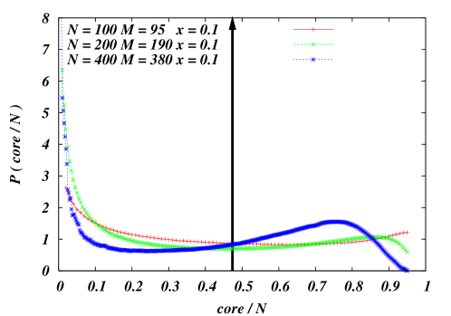
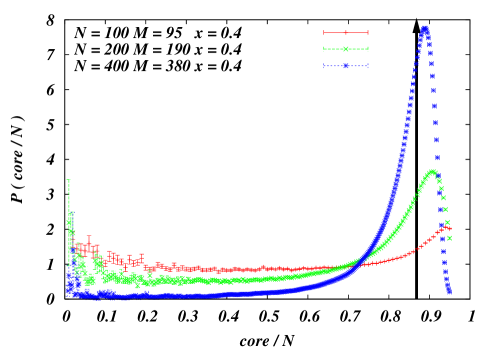
Figure 9: Distribution of core sizes at $\alpha=0.95$ for two different concentration of non-canalizing functions $x=0.0,0.1,0.4$ corresponding respectively to the “first cores” phase (left panel), the “typical core” phase (central panel), and the “all cores overlapping” phase (right panel) respectively (see Fig. 8). The black solid arrows are the theoretical average core density values in the thermodynamic limit for the corresponding $(\alpha,x)$ values as computed in jstat .

.

IV On the random asynchronous dynamics of BN

In the previous sections, we have only analyzed the propagation of external regulation. This last section is dedicated to the full asynchronous update dynamics: Starting from a random assignment to all variables, in every step one function is selected randomly and its output is updated, i.e., it changes its value if and only if the function was unsatisfied before. As before, the time $t=T/M$ is measured by rescaling the number of update attempts $T$ by the number $M$ of all functions, such that in a time-interval of length one each function is visited once on average. In this section we first give an approximate description of the evolution of the number of unsatisfied functions, and at the end we relate the dynamics to the PER core studied before.

IV.1 The energy of canalizing and non-canalizing functions

In order to characterize the asynchronous dynamics we introduce a Hamiltonian which counts the number of unsatisfied Boolean constraints:

$${\cal H}(\vec{s}) = \sum_{a\in INT}s_{a}\oplus F_{a}(s_{a_{1}},...,s_{a_{K}})$$ (34)

$$= [(1-x)\,e_{c}+x\,e_{nc}]M\ .$$

The symbol $\oplus$ stands for the logical XOR operation, i.e. each cost term contributes $0$ to the sum if Eq. (1) is fulfilled, and $1$ otherwise. We have divided this energy into contributions coming from canalizing functions, and those from non-canalizing functions. More precisely, $e_{c}$ stands for the fraction of unsatisfied canalizing functions, $e_{nc}$ for the fraction of unsatisfied non-canalizing functions. In the beginning, all variables take random values. Each function is therefore violated with probability 1/2,

$$e_{c}(t=0)=e_{nc}(t=0)=\frac{1}{2}\ .$$ (35)

Despite some efforts in the last years SeCu ; DYN ; SeWe ; HanWe ; Ha+ , the dynamics of diluted models remains an unsolved problem, and we have to restrict our analysis to approximate methods. Following the ideas of SeWe , and restricting our attention to the simplest level of description, we can close the equations for $e_{c}(t)$ and $e_{nc}(t)$ by assuming that at each step all configurations of given energy values are equally probable DRT . This is clearly an approximate assumption, but it leads to a good quantitative description of the real dynamics.

As in the case of the core evolution, the dynamics leads to simple ordinary differential equations. We first write them down, and then discuss the meaning of all contributions:

$$(1-x)\,\dot{e}_{c} = -(1-x)\,e_{c}+[(1-x)\,e_{c}+x\,e_{nc}]\,\alpha(1-x)(1-2e_{c})$$

$$x\,\dot{e}_{nc} = -x\,e_{nc}+[(1-x)\,e_{c}+x\,e_{nc}]\,2\alpha x(1-2e_{nc})$$ (36)

Let us first discuss the first equation. The prefactor $(1-x)$ on the left-hand side comes from the fact that the time is measured with respect to $M$, whereas $e_{c}$ is a fraction of the $(1-x)M$ canalizing functions. The first term on the right-hand side is the contribution of the selected function itself: With probability $(1-x)$ it is canalizing, and with probability $e_{c}$ it changes from unsatisfied to satisfied, and the energy decreases by one. The second term comes from the functions regulated by the output of the updated functions: With probability $[(1-x)\,e_{c}+x\,e_{nc}]$ the selected function was updated, and thus the dependent functions might change status. There are on average $2\alpha$ such functions, a fraction $(1-x)$ of them being canalizing. They change status only if the other input has not its canalizing value (factor 1/2). The energy goes up for the fraction $(1-e_{c})$ of satisfied functions, and down for the fraction $e_{c}$ of unsatisfied functions. The second equation is similar, with the main difference that the energy status of a non-canalizing function changes always if one input is changed, leading to a relative factor $2$ compared to the canalizing case.

These two equations have the obvious fixed point $e_{c}=e_{nc}=0$. It corresponds to a fixed point of the microscopic dynamics in the sense that all functions are satisfied, and the update dynamics never flips any of the variables. Are there also other, positive-energy solutions? Assuming that a non-zero solution appears continuously, we linearize the fixed point equation

$$0 = -(1-x)\,e_{c}+[(1-x)\,e_{c}+x\,e_{nc}]\,\alpha(1-x)$$

$$0 = -x\,e_{nc}+[(1-x)\,e_{c}+x\,e_{nc}]\,2\alpha x$$ (37)

Adding these two equations, we find that the non-zero solution appears at

$$\alpha=\frac{1}{1+x}\ ,$$ (38)

i.e. at the same point where typically the PER core appears. This transition corresponds to critical BN jstat . For smaller $\alpha$, the system fastly approaches a zero-energy fixed point, the basic mechanism being fixation of almost all variables by PER. Above the transition, the system settles down at positive energy. At least a part of the core variables continues to flip for ever (in the thermodynamic limit).

To confirm this picture, we have numerically integrated Eqs. (IV.1) and in parallel performed direct numerical simulations on large BN. The results are shown in Fig. 10, and confirm the analytical findings. We see, in particular, that the simple approximation already gives a quantitatively good description of the dynamics. Following the ideas of SeWe this result can surely be improved, but doing so goes beyond the scope of the present paper.

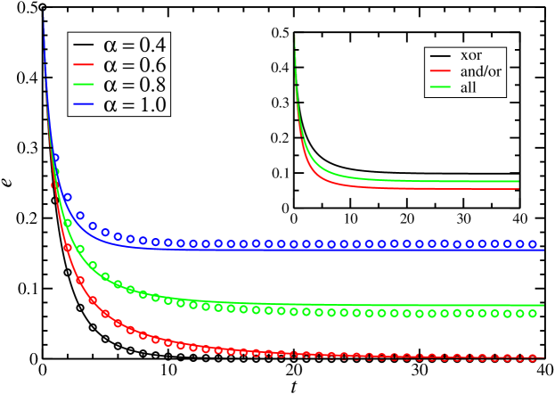
Figure 10: Time evolution of the energy: Approximate analytical description (full lines) vs. numerical simulations (symbols) on single BNs of $N=10^{6}$. The inset shows the different evolution of the energy contributions coming from canalizing and non-canalizing functions.

IV.2 Relating PER and dynamics

In Sec. III we have studied PER also as a dynamical process. In the initial condition all external variables are fixed to some configuration in $\{0,1\}^{N-M}$, whereas internal variables are initially assigned the joker value $\star$. This generalized configuration can be understood as a projection of the set of all $2^{\alpha N}$ initial conditions with fixed external and changeable internal nodes. This consideration makes clear that (for the fixed external configuration) all variables not belonging to the PER core get fixed after ${\cal O}(N\log N)$ elementary steps. Core variables potentially might go on flipping for ever. However, also subsets of core variables could freeze self-consistently due to feedback loops. These subsets depend both on the initial condition of the regulated variables and on the realization of random update dynamics.

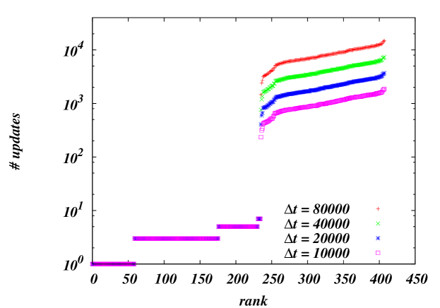
Figure 11: Ranked distribution of the number of elementary spin-updates of the set of variables belonging to the PER core, for $N=1000$, $M=900$, $x=0.2$ and up to 80000 asynchronous updates sweeps (see text). The PER core in this case is made of 408 variables. The 250 first-ranking spins fix their value after $\sim 10$ steps while the remaining spins keep changing their values.

.

To investigate this question, we have analyzed the dynamics restricted to the PER core. We first fixed all non-core variables by PER, note that this can achieved efficiently for any external condition. Then we set the core variables randomly. This slightly atypical choice of initial condition helps to make more evident the dynamics on the core. In the asynchronous dynamics, all these variables (or their regulating function) are on average seen equally often, but they are flipped if and only if the function was not satisfied before. We record the number of actual variable changes for each PER core site, in order to identify frozen versus changeable variables.

In Fig. 11 we display the number of actual spin-flips for each variable during a run of 80000 sweeps (each sweep consisting of $\alpha N$ attempted spin flips). We measure these quantities at different times, namely after $t=10000,20000,40000$ and $80000$ sweeps. We consider a random BN with $N=1000$, $M=\alpha N=900$, $x=0.2$. The configuration of the external inputs is chosen at random and leads to a PER core of 408 variables.

We find two types of behavior: In this sample more than half of the variables become frozen at the very beginning of the dynamics and change only up to about $10$ times. This happens despite the fact that they belong to the core and thus are not fixed by PER. Freezing thus has to appear self-consistently due to feedback loops. The second group of variables goes on changing. The number of their spin-flips grows proportionally to the number of sweeps, as follows from the parallel curves in Fig. 11. After a few sweeps the dynamics becomes concentrated to this second class of variables. Note however that the subdivision of core variables into these two classes depends on the initial condition and the order of the updates which by definition is random. Both identity and number of frozen spins fluctuate from realization to realization, but the qualitative scenario remains the same. It would be very interesting to get a quantitative analytical understanding of this phenomenon.

V Conclusions

In this work we have studied the propagation of external regulatory information into a random Boolean network. The efficiency of this propagation depends on two control parameters: The fraction $(1-\alpha)$ of non-regulated input variables in between all Boolean variables, and the fraction $x$ of non-canalizing variables.

We find that for $\alpha<1/2$ the external condition propagates through the full BN and fixes efficiently all variables. For higher $\alpha$, a fraction of variables remain unfixed by this process, forming thus the PER core of the BN. The precise PER core depends on the external condition. We have studied the fluctuation of the PER core size between different external conditions. Only for $\alpha>1/(1+x)$ the PER core is not empty for almost all external conditions, for even higher $\alpha$ all PER cores start to overlap.

The notion of the PER core is intimately related to the dynamics of the system. After very short time all non-core variables become frozen, so only core variables can be considered as the true dynamical degrees of freedom of the BN under a specified external configuration. However, also a part of the core variables becomes dynamically frozen during the dynamical evolution of the system, the reason being self-consistently fixed feedback loops. The dynamics of the system for longer time scales becomes concentrated on the remaining variables.

In a future work, we plan to extend the PER analysis also to the analytical calculation of the PER core size distribution, which so far we obtained only numerically for small BNs. In this context it would be interesting to algorithmically identify those external conditions which lead to largest or smallest cores. This would help to solve the inverse problem of determining the external conditions leading to a specific core.

A second interesting extension of the current work would be a deepened analysis of the dynamical behavior of this model. In distinction to other models on diluted networks, including in particular diluted spin glasses, BN are defined on directed graphs. This leads to some technical simplifications which we hope to open new ways in the understanding of their dynamical behavior.

References

- (1) S. Kauffman, Journal of Theoretical Biology 22, 437 (1969).
- (2) M. Aldana Gonzalez, S. Coppersmith, and L.P. Kadanoff in Perspectives and Problems in Nonlinear Science, Applied Matematical Science, Springer, (2003).
- (3) E. R. Dougherty, I. Shmulevich, J. Chen, Z. J. Wang, Eds., Genomic Signal Processing and Statistics, EURASIP, (2005).
- (4) S. Kauffman, The Origins of order, Oxford University Press, NY, (1993).
- (5) B. Samuelsson, C. Troein, Phys. Rev. Lett. 90, 098701 (2003).
- (6) U. Bastolla, G. Parisi PHYSICA D, 98, 1 (1997); J. Theoretical Biology, 187, 117, (1997).
- (7) F. Derrida, Y. Pomeau, Europhysics Letters 1, 45 (1986).
- (8) M. Mezard, G. Parisi, and R. Zecchina, Science 297, 812 (2002);
- (9) A. Hartmann, M. Weigt, “Phase Transitions in Combinatorial Optimization Problems”, Wiley-VCH, Berlin, (2005).
- (10) L. Correale, M. Leone, A. Pagnani, M. Weigt, and R. Zecchina, Phys. Rev. Lett. 96, 018101, (2006).
- (11) L. Correale, M. Leone, A. Pagnani, M. Weigt, and R. Zecchina, J. Stat. Mech P03002 (2006).
- (12) Michele Leone, Andrea Pagnani, Giorgio Parisi, Osvaldo Zagordi, J. Stat. Mech. P12012, (2006).
- (13) M. Cosentino Lagomarsino, P. Jona, B. Bassetti, Phys Rev Lett. 95, 15, (2005).
- (14) C. Gershenson, in J. Pollack et al. (ed.), Artificial Life, Proceedings of the Ninth International Conference on the Simulation and Synthesis of Living Systems (MIT Press, 2004).
- (15) F. Greil and B. Drossel, Phys. Rev. Lett. 95, 048701 (2005).
- (16) S. Kauffman, C. Peterson, B. Samuelsson, and C. Troein, PNAS 100, 14796 (2003) and PNAS 101, 17102 (2004).
- (17) M. Mezard, F. Ricci-Tersenghi, and R. Zecchina, J. Stat. Phys. 111, 505 (2003); S. Cocco, O. Dubois, J. Mandler, and R. Monasson, Phys. Rev. Lett. 90, 047205 (2003).
- (18) M. Mézard, G. Parisi, Eur. Phys. Journ. B 20, 217, (2001).
- (19) M. Mézard, G. Parisi, J. Stat. Phys. 111, 1, (2003).
- (20) N. Guelzim, S. Bottani, P. Bourgine, and F. Kèpés, Nat. Gen. 31, 60 (2002).
- (21) R. Albert and H.G. Othmer, Journal of Theoretical Biology 223, 1-18 (2003); q-bio.MN/0312012.
- (22) J.S. Yedidia, W.T. Freeman, Y. Weiss, in Advances in Neural Information Processing Systems, MIT press, 689 (2001).
- (23) F.R. Kschischang, B.J. Frey, H.A. Loeliger, IEEE Transactions on Information Theory, 47, 498, 2001.
- (24) A. Braunstein, M. Mézard, R. Zecchina, Random Structures and Algorithms 27 issue 2, 201 (2005).
- (25) G. Semerjian and L.F. Cugliandolo., Europhys. Lett. 61, 247 (2003).
- (26) G. Semerjian, L.F. Cugliandolo and A. Montanari, J. Stat. Phys. 115, 493 (2004);
- (27) G. Semerjian and M. Weigt, J. Phys. A 37, 5525 (2004).
- (28) H. Hansen-Goos and M. Weigt, J. Stat. Mech., P08001, 2005.
- (29) J.P.L. Hatchett, I. Pérez Castillo, A.C.C. Coolen, and N.S. Skantzos, Phys. Rev. Lett. 95, 117204 (2005).
- (30) A. Montanari and G. Semerjian, Phys. Rev. Lett. 94, 247201 (2005).
- (31) A.C.C. Coolen and D. Sherrington, J. Phys. A 27, 7687 (1994); S.N. Laughton, A.C.C. Coolen, and D. Sherrington, J. Phys. A 29, 763 (1996).