Estimation Diversity and Energy Efficiency in Distributed Sensing

Abstract

Distributed estimation based on measurements from multiple wireless sensors is investigated. It is assumed that a group of sensors observe the same quantity in independent additive observation noises with possibly different variances. The observations are transmitted using amplify-and-forward (analog) transmissions over non-ideal fading wireless channels from the sensors to a fusion center, where they are combined to generate an estimate of the observed quantity. Assuming that the Best Linear Unbiased Estimator (BLUE) is used by the fusion center, the equal-power transmission strategy is first discussed, where the system performance is analyzed by introducing the concept of estimation outage and estimation diversity, and it is shown that there is an achievable diversity gain on the order of the number of sensors. The optimal power allocation strategies are then considered for two cases: minimum distortion under power constraints; and minimum power under distortion constraints. In the first case, it is shown that by turning off bad sensors, i.e., sensors with bad channels and bad observation quality, adaptive power gain can be achieved without sacrificing diversity gain. Here, the adaptive power gain is similar to the array gain achieved in Multiple-Input Single-Output (MISO) multi-antenna systems when channel conditions are known to the transmitter. In the second case, the sum power is minimized under zero-outage estimation distortion constraint, and some related energy efficiency issues in sensor networks are discussed.

I Introduction

Wireless Sensor Networks (WSNs) deploy geographically-distributed sensor nodes to collect information of interest. The collected information is usually aggregated via wireless transmissions at a fusion center to generate the final intelligence. A typical wireless sensor network, as shown in Fig. 1, consists of a fusion center and a number of sensors. The sensors typically have limited energy resources and communication capability. Each sensor in the network makes an observation of the quantity of interest, generates a local signal (either analog or digital), and then sends it to the fusion center where the received sensor signals are combined to produce a final estimate of the observed quantity. Sensor networks of this type are suited for various applications such as environmental monitoring and smart factory instrumentation.

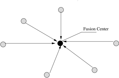
Figure 1: Sensor network with a fusion center.

There has been a long history on the study of distributed estimation. Examples of early work include the study in the context of distributed control [1, 2], tracking [3], or data fusion [4, 5]. Recently, many new results appear in the WSN community with a focus on distributed data fusion, where the most commonly used network fusion model is the one where each sensor processes its individual measurement and transmits the result over a Multiple Access Channel (MAC) to the fusion center. From an information-theoretic perspective, [6, 7, 8, 9, 10] investigate the mean squared estimation error performance versus transmit power for the quadratic CEO problem with a coherent MAC. Notably, it is shown in [6] that if the sensor statistics are Gaussian, a simple uncoded (analog-and-forwarding) scheme dramatically outperforms the separate source-channel coding approach and leads to an optimal asymptotic scaling behavior. The uncoded communication scheme is further proved to preserve the optimal scaling law in [9] for sensor networks with node statistics satisfying a certain mean condition, while the source-channel matching result is extended to more general homogeneous signal fields in [10]. If the sensor measurements are not continuous but in a finite alphabet, type-based transmission schemes are proposed in [11, 12]. The many-to-one transport capacity and compressibility are investigated for dense joint estimation sensor networks in [13]. When a full coordination among sensors is unavailable and the underlying communication links are not reliable, the distributed estimation problem is investigated in [14], where an information-theoretic achievable rate-distortion region is elegantly derived. The work in [15] studies the in-network processing approaches based on a hierarchical data-handling and communication architecture for the estimation of field sources. In addition, by assuming only local sensor information exchange, [16] proposes a distributed algorithm for reaching network-wide consensus.

Among most of the existing studies, it is usually assumed that the joint distribution of the sensor observations is known. However, in some practical systems the probability density function (pdf) of the observation noise is hard to characterize, especially for a large scale sensor network. This motivates us to devise universal signal processing algorithms that do not require the knowledge of the observation noise distributions. Recently, universal Decentralized Estimation Schemes (DESs) are proposed in [17] and [18]. In [17], the author considers the universal distributed estimation in a homogeneous sensor network where sensors have observations of the same quality, while in [18], the universal DES in an inhomogeneous sensing environment is considered. These proposed DESs require each sensor to send to the fusion center a short discrete message with length determined by the local Signal to Noise Ratio (SNR), which then guarantees that the performance is within a constant factor of that achieved by the Best Linear Unbiased Estimator (BLUE). An assumption in these proposed schemes is that the channels between the sensors and the fusion center are perfect, i.e., all messages are received by the fusion center without any distortion. However, due to power limitations, fading, and channel noise, the signal sent by each individual sensor to the fusion center may be corrupted. Therefore, the transmission system for the joint estimation scheme should be designed to minimize the end-to-end distortion subject to certain transmit power constraints, under a practical wireless channel model considering both fading and additive noises. In this paper we show that in a fading wireless environment, multiple sensor nodes are not only necessary for generating multiple observations to reduce distortion, but also crucial to achieve a certain degree of diversity that minimizes the effects of fading during signal transmissions.

If the sensor observation is in analog form, we have two main options to transmit the observations from sensors to the fusion center: analog or digital. For the analog approach, the observed signal is transmitted via analog modulation to the fusion center, which we refer to as the amplify-and-forward approach. In the digital approach, the observed signal is digitized into bits, possibly compressed and/or encoded, then digitally modulated and transmitted. It is well known ([19], [20]) that for a single Gaussian source with an Additive White Gaussian Noise (AWGN) channel, both the digital and analog approaches can retain the optimal power-distortion tradeoff. Also for the estimation of a Gaussian source with a coherent Gaussian MAC, it is shown in [6, 9, 10] that the analog forwarding schemes outperform (or are as good as) the digital approaches and have the optimal asymptotic scaling behavior. For sources with general distributions, type-based (each sensor transmits the local type or histogram of its data in an analog fashion over a MAC) parametric estimation schemes are proposed in [9, 11, 12]. In the above papers, the impact of coherent MAC schemes on the joint source-channel optimality is discussed.

In this paper, instead of assuming a coherent MAC, we adopt orthogonal channels between the sensors and the fusion center. The main motivation for using orthogonal multiple access schemes such as Frequency Division Multiple Access (FDMA) is the removal of the requirement on the carrier-level synchronization among sensors (we still require pair-wise synchronization between each sensor and the fusion center). We assume that the observed signal is analog and the observation noises are uncorrelated across sensors. In addition, we assume that the second moments of the signal and noise are known to the corresponding sensor and the fusion center. The fusion center deploys the best linear unbiased estimator to generate estimates of the unknown signal. In this setting, we investigate an analog transmission system where observations are amplified and forwarded to the fusion center. We first analyze the system performance in fading channels by introducing the concept of estimation diversity. We investigate the diversity gain that is achievable in a slow fading environment, where it is assumed that the transmission between sensors and the fusion center experiences i.i.d. fading factors together with AWGNs. An outage is claimed if the end-to-end distortion is larger than a certain threshold. In this case, we show that using multiple sensors can achieve diversity to enhance the outage performance, where the diversity order is equal to the total number of sensors. We then find the optimal power allocation strategy for the case where the end-to-end distortion is minimized under certain transmit power constraints. The result leads to turning off certain sensors with bad channels and bad observation quality. By doing so, the achievable diversity order is not reduced and extra adaptive power gain is obtained. We finally investigate the converse problem to minimize the total power consumption under a certain distortion constraint.

The rest of the paper is organized as follows. Section II discusses the system model. Section III analyzes the distortion performance of an equal-power transmission strategy, where the concept of estimation diversity is introduced. Section IV addresses the case where the transmission power is allocated in an optimal way to minimize the distortion. Section V focuses on the converse case where power is minimized subject to a distortion constraint. Section VI summarizes the results and presents our conclusions.

II System Model

We assume a sensor network with $K$ sensors where the observation $x_{k}(t)$ at sensor $k$ is represented as a random signal $\theta(t)$ corrupted by observation noise $n_{k}(t)$: $x_{k}(t)=\theta(t)+n_{k}(t)$, $t=0,1,2,\cdots$. We also assume that both $\theta(t)$ and $n_{k}(t)$ are i.i.d. over time $t$. Each sensor transmits the signal $x_{k}(t)$ to the fusion center where $\theta(t)$ is estimated from the received version of $x_{k}(t)$’s, $k=1,\cdots,K$. We further assume that $\theta(t)$ and $n_{k}(t)$ have zero mean and second moments $\sigma_{\theta}^{2}$ and $\sigma_{k}^{2}$ respectively, based on which we define the local observation SNR for sensor $k$ as: $\gamma_{k}=\sigma_{\theta}^{2}/\sigma_{k}^{2}$.

We assume that $K$ sensors transmit their observations to the fusion center via $K$ orthogonal channels (FDMA), where different channels experience independent fading factors and zero-mean AWGNs. Specifically, for channel $k$, we assume i.i.d. (over $t$) block fading with the channel power gain denoted as $g_{k}(t)$, and i.i.d. (over $t$) AWGNs denoted as $n_{ck}(t)$ of variance $\xi_{k}^{2}$, $k=1,\cdots,K$, where the variances are assumed to be the same for all $k$’s in this paper. We also assume pair-wise synchronization between each sensor and the fusion center. However, synchronization among sensor nodes is not required. At each sensor transmitter, we adopt an analog amplify and forward uncoded strategy, motivated by the results derived in [20]. Therefore, at sensor $k$, the transmitter can be simply modeled by a power amplifying factor $\alpha_{k}(t)$ and the average transmit power is given as

$$P_{k}=\alpha_{k}{P_{x_{k}}}=\alpha_{k}(\sigma_{\theta}^{2}+\sigma_{k}^{2})=\alpha_{k}^{\prime}(1+\gamma_{k}^{-1})$$ (1)

where $P_{x_{k}}$ is the average power of $x_{k}(t)$ and $\alpha_{k}^{\prime}=\alpha_{k}\sigma_{\theta}^{2}$. Note that we only need to consider the power gains (no phase information is needed) in both the transmitter and the channel, based on the assumptions that only the amplitude of $\theta(t)$ is estimated and coherent reception (the effect of phase is eliminated due to synchronization) is performed in the fusion center for each $x_{k}(t)$.

Given the assumption of system independence over time $t$, we can analyze the system performance by first focusing on an arbitrary time snapshot, and then apply the result (which is conditional on one system realization) to analyze the long-term average and outage performance in the later sections. Therefore, from now on we neglect the time index $t$ in all the parameters. The overall system structure at one snapshot is shown in Fig. 2.

\psfrag{theta}{$\theta$}\psfrag{b1}{$\sqrt{\alpha_{1}}$}\psfrag{b2}{$\sqrt{\alpha_{2}}$}\psfrag{bK}{$\sqrt{\alpha_{K}}$}\psfrag{a1}{$\sqrt{g_{1}}$}\psfrag{a2}{$\sqrt{g_{2}}$}\psfrag{aK}{$\sqrt{g_{K}}$}\psfrag{n1}{$n_{1}$}\psfrag{n2}{$n_{2}$}\psfrag{n3}{$n_{K}$}\psfrag{nc1}{$n_{c1}$}\psfrag{nc2}{$n_{c2}$}\psfrag{ncK}{$n_{cK}$}\psfrag{yk}{$y_{1},\cdots,y_{K}$}\includegraphics[width=216.81pt,height=101.17755pt]{fig2.eps}

Figure 2: Amplify and forward

The received signal vector is given by

$$\mathbf{y}=\mathbf{h}\theta+\mathbf{v},$$ (2)

where

$$\mathbf{y} = \left[y_{1},y_{2},\cdots,y_{K}\right]^{{\dagger}},$$

$$\mathbf{h} = \left[{\sqrt{\alpha_{1}g_{1}}},{\sqrt{\alpha_{2}g_{1}}},\cdots,{\sqrt{\alpha_{K}g_{K}}}\right]^{{\dagger}},$$

$$\mathbf{v} = \left[{\sqrt{\alpha_{1}g_{1}}}n_{1}+n_{c1},\cdots,{\sqrt{\alpha_{K}g_{K}}}n_{k}+n_{cK}\right]^{{\dagger}},$$

with ${\dagger}$ denoting transposition.

Since we intend to make the estimator universal (independent of particular observation noise distributions except the second-order statistics) and simple, the BLUE [21] is adopted at the fusion center. Accordingly, the estimate for $\theta$ conditional on a given set of channel gains is given by

$$\hat{\theta} = [\mathbf{h}^{{\dagger}}\mathbf{R}^{-1}\mathbf{h}]^{-1}\mathbf{h}^{{\dagger}}\mathbf{R}^{-1}\mathbf{y}$$ (3)

$$= \left(\sum_{k=1}^{K}\frac{{\alpha_{k}g_{k}}}{\sigma_{k}^{2}{\alpha_{k}g_{k}}+\xi_{k}^{2}}\right)^{-1}\sum_{k=1}^{K}\frac{{\sqrt{\alpha_{k}g_{k}}}y_{k}}{\sigma_{k}^{2}{\alpha_{k}g_{k}}+\xi_{k}^{2}},$$

where the noise variance matrix $\mathbf{R}$ is a diagonal matrix with $R_{kk}={\sigma_{k}^{2}{\alpha_{k}}{g_{k}}+\xi_{k}^{2}}$, $k=1,\cdots,K$.

The Mean Squared Error (MSE) of this estimator is given as [21]

$${\rm Var}[\hat{\theta}] = [\mathbf{h}^{{\dagger}}\mathbf{R}^{-1}\mathbf{h}]^{-1}$$ (4)

$$= \left(\sum_{k=1}^{K}\frac{{\alpha_{k}g_{k}}}{\sigma_{k}^{2}{\alpha_{k}g_{k}}+\xi_{k}^{2}}\right)^{-1}$$

$$= \sigma_{\theta}^{2}\left(\sum_{k=1}^{K}\frac{{\alpha_{k}^{\prime}s_{k}}}{\gamma_{k}^{-1}{\alpha_{k}^{\prime}s_{k}}+1}\right)^{-1},$$

where for notational convenience, we introduce the channel SNR: $s_{k}={g_{k}}/{\xi_{k}^{2}}$, $k=1,\cdots,K$.

We now summarize the notations that we have defined so far (for a particular time snapshot).

• $\theta$ and $\sigma_{\theta}^{2}$: Signal to estimate and its variance;

• $n_{k}$ and $\sigma_{k}^{2}$: Observation noise and the associated variance at sensor $k$;

• $x_{k}$: Observation signal at sensor $k$;

• $\alpha_{k}$: Power amplifying factor at sensor $k$; In addition, $\alpha_{k}^{\prime}:=\alpha_{k}\sigma_{\theta}^{2}$;

• $g_{k}$: Power gain of channel $k$;

• $n_{ck}$ and $\xi_{k}^{2}$: Zero-mean AWGN of channel $k$ and its variance, with $\xi_{k}^{2}$ the same for all $k$’s;

• $\gamma_{k}:=\sigma_{\theta}^{2}/\sigma_{k}^{2}$: Local observation SNR at sensor $k$;

• $s_{k}:={g_{k}}/{\xi_{k}^{2}}$: SNR of channel $k$.

III equal-power Allocation: Estimation Diversity

Given the proposed joint estimation system, we are interested in investigating how the overall distortion performance is affected by the fact that we have multiple sensors with independent fading channels. We first investigate how the average distortion scales with the number of sensors in the network, and secondly, we quantify how the reliability of the overall estimation system is enhanced as we increase the number of sensors given independent observations and independent fading channels across different sensors.

To assure fairness when we compare different systems with different numbers of sensor nodes, we fix the total transmission power that the $K$ nodes can use, denoted as $P_{tot}$. In this section, we consider the case of equal-power allocation where all sensors transmit the same amount of power. As the total power budget for all sensors is $P_{tot}$, according to Eq. (1), we have

$$\alpha_{k}^{\prime}=\frac{P_{tot}}{K{(1+\gamma_{k}^{-1})}},\quad 1\leq k\leq K.$$

According to Eq. (4), the achieved MSE is

$${\rm Var}[\hat{\theta}]=\sigma_{\theta}^{2}\left(\sum_{k=1}^{K}\frac{{P_{tot}s_{k}}}{\gamma_{k}^{-1}{P_{tot}s_{k}}+K(1+\gamma_{k}^{-1})}\right)^{-1}.$$ (5)

We assume that the channels between sensors and the fusion center experience channel gain $g_{k}$’s, which are i.i.d. over $k$, and the sensors have different observation noises with random variances $\sigma_{k}^{2}$’s that are also i.i.d. over $k$. The i.i.d. assumption on $\sigma_{k}^{2}$’s can be justified if we assume that the sensors are randomly deployed into the field and the different measurement noise variances are caused by different observation distances. With these assumptions, we observe that both $\gamma_{k}$’s and $s_{k}$’s are i.i.d. over $k$, and without loss of generality we have $E(\gamma_{k})=E(\gamma_{1})$ and $E(s_{k})=E(s_{1})$, $k=1,\cdots,K$.

Our first question is: Suppose that the total power $P_{tot}$ is fixed; what is the asymptotic behavior of ${\rm Var}[\hat{\theta}]$ when the total number of sensors K increases without bound?

When $s_{k}$’s and $\gamma_{k}$’s are random and i.i.d. over $k$, we have

$$\lim_{K\rightarrow\infty}{\rm Var}[\hat{\theta}]=\frac{\sigma_{\theta}^{2}}{P_{tot}E[s_{1}/(1+\gamma_{1}^{-1})]}:=D_{\infty},$$ (6)

for which the derivation is given in Appendix A.

From the result in Eq. (6) and the corresponding derivation given in Appendix A, we conclude the following:

• With a finite amount of total transmit power $P_{tot}$ for all the sensors, the overall MSE ${\rm Var}[\hat{\theta}]$ does not decrease to zero even if $K$ approaches infinity. This is a consequence of using orthogonal links from the sensors to the fusion center, which leads to $K$ different channel noises such that the corruption of channel noise cannot be eliminated even when $K$ goes to infinity. Systems based on non-orthogonal multiple access schemes are discussed in  [25, 26], where it is shown that with finite total transmit power, ${\rm Var}[\hat{\theta}]$ can be driven to zero when $K$ goes to infinity. However, in those systems perfect carrier synchronization among all the sensor nodes and full channel knowledge (amplitude gain and phase shift) at the transmitters are required, which may not be feasible in practical systems.

• Although ${\rm Var}[\hat{\theta}]$ is bounded away from zero, it decreases monotonically with $K$. However, the reduction in distortion with each additional sensor decreases as $K$ gets large (c.f. Eq. (29));

• When $K$ is large, ${\rm Var}[\hat{\theta}]$ is inversely proportional to $P_{tot}$. Thus, when $K$ increases, if $P_{tot}$ also increases (at any speed) with $K$, we have $D_{\infty}=0$.

This analysis suggests that when the total amount of power $P_{tot}$ is fixed, even though the total number of sensors $K$ increases without bound, the achieved average distortion at the fusion center does not decrease below a certain level $D_{\infty}$. However, are there any benefits of having more sensors in the network if we limit the amount of total power? To answer this question, let us define the outage probability ${\mathcal{P}_{D_{0}}}$ to model the system reliability as follows,

$$\mathcal{P}_{D_{0}}={\rm Prob}\{{\rm Var}[\hat{\theta}]>D_{0}\},$$ (7)

where $D_{0}$ is a predefined threshold. Given the i.i.d. nature of $s_{k}$’s and $\gamma_{k}$’s, the probability of ${\rm Var}[\hat{\theta}]>D_{0}$ at one particular snapshot is an appropriate indicator of the long-term estimation system reliability. The following theorem summarizes the relationship among $\mathcal{P}_{D_{0}}$, $P_{tot}$, and the number of sensors $K$.

Theorem III.1

Suppose sensor observation SNR $\{\gamma_{k}:k=1,2,\ldots,K\}$ and channel SNR $\{s_{k}:k=1,2,\ldots,K\}$ are both i.i.d. across $k$. Define $\eta_{k}:=s_{k}/(1+\gamma_{k}^{-1})$. In addition, we assume that $E[\eta_{k}]$ and $E[\gamma_{k}^{-1}{s_{k}^{2}}]$ are finite. When the total number of sensors $K$ is large, with the total power $P_{tot}$ and equal-power allocation among sensors, we have the achievable average distortion

$$D_{\infty}:=\lim_{K\rightarrow\infty}{\rm Var}[\hat{\theta}]=\frac{\sigma_{\theta}^{2}}{P_{tot}E[\eta]}.$$

Moreover, for a sufficiently large but finite $K$ and $D_{0}>D_{\infty}$, we have the outage probability (c.f. Eq. (7))

$${\mathcal{P}_{D_{0}}}\sim\exp(-KI_{\eta}(a)),\hskip 5.69046pt\mbox{or}\hskip 5.69046pt-\log{\mathcal{P}_{D_{0}}}\sim{KI_{\eta}(a)},$$

where $\sim$ means asymptotically converging to (as $K$ becomes large), $\eta$ is the common distribution of $\eta_{k}$, $a=\sigma_{\theta}^{2}/(D_{0}P_{tot})$, and $I_{\eta}(a)$ is the rate function of $\eta$:

$$I_{\eta}(a)=\sup_{\theta\in\mathbb{R}}(\theta a-\log M_{\eta}(\theta)),$$

with $M_{\eta}(\theta)$ the moment generating function of $\eta$.

A more detailed explanation of the rate function and the proof of Theorem III.1 are given in Appendix B.

From the theorem we see that $K$ plays the role of estimation diversity order here, in that the outage probability decreases exponentially with K. We remark that the fact that the outage probability decays exponentially with the number of sensors is due to the effect of independent measurements and fading coefficients, which bears similar properties as the probability of detection error in distributed detection [22, 23, 12, 24]. Note that even though Theorem III.1 is an asymptotic result for large $K$, we later show by simulation results that the outage probability curve illustrates diversity order of $K$ (approximately) even for small values of $K$ in practical scenarios.

As an example, let us consider the case in which $\gamma_{k}=1$ for $k$’s and $\sqrt{s_{k}}$ is i.i.d. Rayleigh with pdf

$$f_{\sqrt{s}}(x)=\frac{x}{\delta^{2}}\exp\left\{-\frac{x^{2}}{2\delta^{2}}\right\}.$$

Then $\eta_{k}=s_{k}/2$ has exponential distribution with pdf

$$f_{\eta}(x)=\frac{1}{\delta^{2}}\exp\left\{-\frac{x}{\delta^{2}}\right\}.$$

Therefore, $E[\eta_{k}]=\delta^{2}$. Thus the achieved asymptotic distortion when $K$ is large is given by

$$D_{\infty}=\lim_{K\rightarrow\infty}{\rm Var}[\hat{\theta}]=\frac{\sigma_{\theta}^{2}}{P_{tot}E[\eta_{k}]}=\frac{\sigma_{\theta}^{2}}{P_{tot}\delta^{2}}.$$

Now we calculate the rate $I_{\eta}(a)$. It is easy to see that the moment generating function of an exponentially distributed random variable with mean $b$ is given as

$$M(\theta)=\frac{1}{1-b\theta}.$$

Thus

$$I_{\eta}(a) = \sup_{\theta\in\mathbb{R}}\left[\theta a+\log(1-b\theta)\right]$$

$$= \frac{a}{b}-\log\frac{a}{b}-1$$

$$= \frac{\sigma_{\theta}^{2}}{\delta^{2}D_{0}P_{tot}}-\log\frac{\sigma_{\theta}^{2}}{\delta^{2}D_{0}P_{tot}}-1,$$

where in the last step, we substituted the expressions $a=\sigma_{\theta}^{2}/(D_{0}P_{tot})$ and $b=\delta^{2}$. When $P_{tot}$ is large, i.e., when $\displaystyle\frac{\sigma_{\theta}^{2}}{\delta^{2}D_{0}P_{tot}}\ll 1$, this leads to

$$I_{\eta}(a) = \frac{\sigma_{\theta}^{2}}{\delta^{2}D_{0}P_{tot}}-\log\frac{\sigma_{\theta}^{2}}{\delta^{2}D_{0}P_{tot}}-1$$

$$\sim \log P_{tot},$$

which means that the estimation convergence rate is approximately $\log{P_{tot}}$ when $\displaystyle\frac{\sigma_{\theta}^{2}}{\delta^{2}D_{0}P_{tot}}\ll 1$ is satisfied. In other words, for Rayleigh fading channels we have

$$-\log{\mathcal{P}_{D_{0}}}\sim K\log P_{tot},$$ (8)

which shows that the diversity order $K$ is the slope of the outage probability vs. power curve if things are plotted in the log-log fashion.

We now provide some numerical examples to verify the analytical results. We assume that the channel SNR is given as $s_{k}=\frac{G_{0}}{\xi_{k}^{2}d_{k}^{2}}|r_{k}|^{2}$ where $d_{k}$ is the transmission distance from sensor $k$ to the fusion center, $G_{0}=-30$ dB is the nominal gain at $d_{k}=1$ m, and the $|r_{k}|$’s are i.i.d. Rayleigh fading random variables with unit variance. We take $\xi_{k}^{2}=-90$ dBm, $k=1,\cdots,K$. To emphasize the possible diversity gain enabled by the independent channel fading values, we set $d_{k}=100$ m and $\sigma^{2}_{k}=0.01$ for all $k$. In addition, we set $\sigma_{\theta}^{2}=1$. The outage threshold $D_{0}$ is set as $D_{0}=2\sigma^{2}_{k}=0.02$.

The end-to-end distortion performance, averaged over random channel gains, is plotted in Fig. 3 for different numbers of sensors, where each point is a sample average over one million independent random channel samples. It is not surprising that the average distortion decreases as we increase the total power budget. Note that the average distortion barely improves when we increase the number of nodes from $3$ to $30$, which matches the comments given after Eq. (6). However, this does not mean that the 3-node case performs as well as the 30-node case, since the average performance is not a good criterion to use in a slow fading environment, where the outage performance is more informative.

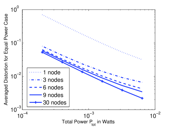
Figure 3: Average Distortion vs. Total Power

The outage probability versus the total transmission power is plotted in Fig. 4 for different numbers of sensors, where we see that the 3-node case performs much better than the 1-node case and the 9-node case performs much better than the 3-node case. Approximately, when the logarithm of outage probability is plotted versus the logarithm of total transmission power, the slope of the curve at the high power region is proportional to the number of sensors, which is defined as the diversity order in Eq. (8). Note that this definition of diversity order is based on the distortion outage performance, which is different from the traditional definition of diversity order in Multiple-Input Multiple-Output (MIMO) multi-antenna systems [31], which is usually the slope of symbol error curves. However, the two definitions imply similar performance benefits from diversity. This type of diversity gain is also shown for large numbers of sensors in Fig. 5, where we see that for the same $D_{0}=0.02$ threshold, the slope of the 20-node curve is twice that of the 10-node curve in the high power region. Not surprisingly, when we decrease $D_{0}$ (down to $0.015$ as shown in Fig. 5), the outage probability will be increased. It is worth mentioning that since $D_{\infty}$ decreases with $P_{tot}$, when $P_{tot}$ increases, a fixed $D_{0}$ becomes progressively conservative as it gets further away from $D_{\infty}$. As such, a more appropriate definition for the outage probability may be $P_{\epsilon}={\rm Prob}\{{\rm Var}[\hat{\theta}]>(1+\epsilon)D_{\infty}\}$ (as pointed out by one of the reviewers), which is definitely worth further investigation, but beyond the scope of this paper.

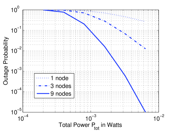
Figure 4: Outage Probability vs. Total Power

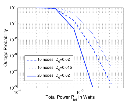
Figure 5: Outage Probability vs. Total Power for Large Numbers of Sensors

IV Optimal power Allocation: Diversity Gain + Power Gain

In the previous section we showed that diversity gain can be achieved even if we use a simple uniform power allocation scheme. In this section, we optimize power allocation among the sensors to minimize the total distortion. The diversity performance is analyzed and we show that a certain adaptive power gain can be achieved by optimal power control. To clarify the analysis, we first discuss the problem with only a sum power constraint, then discuss the general case with both sum and individual power constraints.

IV-A Optimal power allocation with a sum power constraint

With a sum power constraint, the minimum distortion joint estimation problem for each given set of channel gains can be cast as

$$\min {\rm Var}[\hat{\theta}]$$

s. t. $$\sum_{k=1}^{K}P_{k}\leq P_{tot},$$

where $P_{tot}$ is the total power constraint across all the nodes. With Eqs. (1) and (4), we can rewrite the above problem as

$$\min_{\alpha_{k}^{\prime}} \sigma_{\theta}^{2}\left(\sum_{k=1}^{K}\frac{{\alpha_{k}^{\prime}s_{k}}}{\gamma^{-1}\alpha_{k}^{\prime}s_{k}+1}\right)^{-1}$$

s. t. $$\sum_{k=1}^{K}\alpha_{k}^{\prime}{(1+\gamma_{k}^{-1})}\leq{P_{tot}}$$

$${\alpha_{k}^{\prime}}\geq 0,\hskip 8.5359ptk=1,\cdots,K.$$

Our goal is to obtain the optimal power allocation, i.e., optimal $\alpha^{\prime}_{k}$’s. To simplify the objective function, we rewrite the problem as

$$\min_{\alpha_{k}^{\prime}} -\sum_{k=1}^{K}\frac{{\alpha_{k}^{\prime}s_{k}}}{\gamma_{k}^{-1}{\alpha_{k}^{\prime}s_{k}}+1}$$

s. t. $$\sum_{k=1}^{K}\alpha_{k}^{\prime}{(1+\gamma_{k}^{-1})}\leq{P_{tot}},$$

$${\alpha^{\prime}_{k}}\geq 0,\hskip 8.5359ptk=1,\cdots,K.$$

For nonnegative $\alpha_{k}^{\prime}$, it can be shown that the second derivative with respect to $\alpha_{k}^{\prime}$ of each item in the objective function is nonnegative. Since the objective function is also separable over $\alpha_{k}^{\prime}$ (no coupled terms over different $k$’s), it is jointly convex over all the $\alpha^{\prime}_{k}$’s. In addition, all the constraints are linear constraints. Thus, the problem is convex.

Now we solve the problem in Eq. (IV-A). Its Lagrangian $G$ is given as

$$G(\alpha_{k}^{\prime};\lambda_{0},\mu_{k}) = -\sum_{k=1}^{K}\frac{{\alpha_{k}^{\prime}s_{k}}}{\gamma_{k}^{-1}{\alpha_{k}^{\prime}s_{k}}+1}$$

$$-\lambda_{0}\left({P_{tot}}-\sum_{k=1}^{K}\alpha_{k}^{\prime}{(1+\gamma_{k}^{-1})}\right)-\sum_{k=1}^{K}\mu_{k}\alpha^{\prime}_{k}$$

which leads to the following Karush-Kuhn-Tucker (KKT) conditions [29]:

$$-\frac{s_{k}^{-1}}{\left(\gamma_{k}^{-1}\alpha^{\prime}_{k}+s_{k}^{-1}\right)^{2}}+\lambda_{0}{(1+\gamma_{k}^{-1})}-\mu_{k}=0, \forall{k},$$

$$\sum_{k=1}^{K}\alpha_{k}^{\prime}{(1+\gamma_{k}^{-1})}-{P_{tot}}=0,$$

$$\mu_{k}\alpha_{k}^{\prime}=0 \forall{k},$$

$$\mu_{k}\geq 0 \forall{k},$$

$$\alpha_{k}^{\prime}\geq 0 \forall{k}.$$

From the first equation in the above set we obtain

$$-\frac{s_{k}^{-1}}{\left(\gamma_{k}^{-1}\alpha^{\prime}_{k}+s_{k}^{-1}\right)^{2}}+\lambda_{0}{(1+\gamma_{k}^{-1})}=\mu_{k},$$

which leads to the solution

$$\alpha_{k}^{\prime} = \frac{\gamma_{k}}{s_{k}}\left(\frac{1}{\sqrt{s_{k}^{-1}\left(\lambda_{0}{(1+\gamma_{k}^{-1})}-\mu_{k}\right)}}-1\right).$$

Also we can see from the third equation that for those sensors with $\alpha_{k}^{\prime}>0$ (i.e., $P_{k}>0$), $\mu_{k}=0$ holds. Therefore,

$$\alpha_{k}^{\prime} = \frac{\gamma_{k}}{s_{k}}\left(\frac{1}{\sqrt{s_{k}^{-1}\lambda_{0}{(1+\gamma_{k}^{-1})}}}-1\right)^{+}$$ (10)

$$= \frac{\gamma_{k}}{s_{k}}\left(\sqrt{\frac{\eta_{k}}{\lambda_{0}}}-1\right)^{+},\forall{k},$$

where $(x)^{+}$ equals $0$ when $x$ is less than zero, and otherwise equals $x$. The first equality follows from the fact that if $\alpha_{k}^{\prime}>0$, $\mu_{k}=0$, and if $\alpha_{k}^{\prime}=0$, then removing $\mu_{k}$ results in the difference within the bracket being non-positive.

The Lagrangian multiplier $\lambda_{0}$ in Eq. (10) and the number of active sensors (that are assigned non-zero power) can be uniquely determined from the power constraint by the following two-step derivation.

• First, let us assume that only the first $K_{1}$ sensors are active such that $\lambda_{0}$ can be solved by substituting $[\alpha_{1}^{\prime},\cdots,\alpha_{K_{1}}^{\prime}]$ back to the second KKT condition. This assumption can be guaranteed by ranking the sensors (according to $\eta_{k}$ that is a function of both the observation SNR and channel SNR) such that

  $$\eta_{1}\geq\eta_{2}\geq\ldots\geq\eta_{K},$$ (11)

  and the fact that $\alpha_{k}^{\prime}=0$ if $\eta_{k}\leq\lambda_{0}$. As such, we obtain

  $$\lambda_{0}=\left(\frac{A(K_{1})}{B(K_{1})}\right)^{2},$$

  where for any $1\leq k\leq K$,

  $$A(k) = \displaystyle\sum_{m=1}^{k}\frac{\gamma_{m}}{\sqrt{\eta_{m}}}$$

  $$B(k) = \displaystyle\sum_{m=1}^{k}\frac{\gamma_{m}}{\eta_{m}}+P_{tot}.$$

• Secondly, we substitute $\lambda_{0}$ back to Eq. (10) and solve the cutoff index $K_{1}$, which is obviously determined by the relative magnitudes between $\sqrt{\frac{\eta_{k}}{\lambda_{0}}}$ and $1$. Naturally, we introduce the notation:

  $$f(k) = \sqrt{\frac{\eta_{k}}{{\lambda_{0}}}}-1$$ (12)

  $$= \frac{\sqrt{\eta_{k}}B(k)}{A(k)}-1,\quad\mbox{for\ }1\leq{k}\leq{K}.$$

  It follows from Eqns. (10) and (12) that solving the threshold $K_{1}$ is equivalent to finding $K_{1}$ such that $f(K_{1})>0$ and $f(K_{1}+1)\leq 0$. Using the same techniques as in [30, Appendix B], we can show that such a $K_{1}$ is unique and always exists unless $f(k)>0$ for all $1\leq k\leq K$, in which case we take $K_{1}=K$ that means all sensors being active.

Hence, it follows from Eq. (10) that

$${\alpha^{\prime}_{k}}^{opt}=\left\{\begin{array}[]{ll}0,&k>K_{1}\\ \displaystyle\frac{\gamma_{k}}{s_{k}}\left(\sqrt{\eta_{k}}c_{0}-1\right),&k\leq K_{1},\end{array}\right.$$ (15)

where $c_{0}=\sqrt{\lambda_{0}^{-1}}=B(K_{1})/A(K_{1})$. It is easy to see that $c_{0}$ defines the threshold of the $\eta_{k}$’s (i.e., $\eta_{k}\geq{1/c_{0}^{2}}$), by which we can decide whether a sensor transmits or keeps silent. Note that the figure of merit $\eta_{k}=s_{k}/(1+\gamma_{k}^{-1})$ is jointly defined by the channel SNR and local observation SNR. For sensors with low $\eta_{k}$, they are completely shut off and no power is wasted. For the remaining active sensors, power should be assigned according to Eq. (15).

To implement the described optimal power scheduling scheme, the fusion center needs to calculate and broadcast the threshold $\lambda_{0}$ to all the sensors. Each sensor then decides the optimal transmit power according to its own local information ($\gamma_{k}$ and $s_{k}$) and $\lambda_{0}$. Such a power scheduling scheme is feasible when there exists a feedback broadcast channel (of low rate) from the fusion center to each sensor and the channel changes slowly.

Furthermore, according to Eq. (4), the total distortion is given by

$${\rm Var}[\hat{\theta}]=\sigma_{\theta}^{2}\left(\sum_{k=1}^{K_{1}}\gamma_{k}\left(1-\frac{1}{c_{0}\sqrt{\eta_{k}}}\right)\right)^{-1},$$ (16)

and the outage probability can be rewritten as

$${\mathcal{P}_{D_{0}}}={\rm Prob}\left\{\sum_{k=1}^{K_{1}}\gamma_{k}\left(1-\frac{1}{c_{0}\sqrt{\eta_{k}}}\right)<\frac{\sigma_{\theta}^{2}}{D_{0}}\right\}.$$ (17)

To obtain closed-form representations for the outage probability is difficult. However, we can numerically evaluate the performance for the optimal power transmission schemes, and compare it with the closed-form solution developed for the equal-power case in the previous section. Since equal-power allocation is just one feasible solution of the optimization problem in Eq. (IV-A), the resulting optimal solution (which may turn off bad sensors) leads to strictly-lower distortion than the equal-power allocation strategy. Given that we have theoretically shown that the equal-power allocation strategy achieves full estimation diversity (on the order of $K$), we can state that the optimal power allocation strategy performs at least equally well, i.e., achieves full estimation diversity. This is further illustrated by the following simulation results.

We assume that the related system parameters are set the same as in the equal-power case in Section III. In Fig. 6, we plot the percentage of active sensors versus the total transmission power, where we set $K=100$ in the simulation. We note that the number of active sensors can be less than $K$ when the total power budget is small. In Fig. 7, we compare the outage performance of the optimal power scheme with the case where all the sensors transmit with equal power. From the outage probability curves, we see that for the same number of sensor nodes the curve slopes are almost the same for both the equal-power and the optimal power cases, which means that the optimal power transmission strategy achieves the same diversity order of $K$. In addition, the curve for the optimal power case is a left-shifted version of that for the equal-power case. This shift is a result of adaptive power gain that is due to the optimal power control. This gain is similar to array or coding gain in traditional MIMO systems [31].

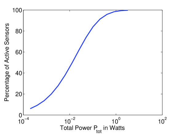
Figure 6: Percentage of Active Sensors vs. Total Power

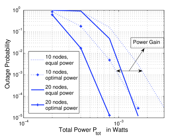
Figure 7: Outage Probability Comparison vs. Total Power

IV-B Optimal power allocation with both sum and individual power constraints

In the optimization problem of Eq. (IV-A), the sum power constraint is imposed to guarantee a fair comparison when we change the number of sensor nodes. In some application scenarios, this sum power constraint has a physical meaning. For example, let us assume that there are multiple clusters of sensors, where each cluster is performing a different observation task. If different clusters are sharing the same frequency band to transmit information, the total power emitted from each cluster must be limited to enable the coexistence of multiple clusters. In addition, a more severe power constraint may be imposed on each individual sub-band used by each sensor for better frequency reuse, which is modeled by individual power constraints for all the sensors. Note that the individual power constraint may also be imposed by power supply characteristics at each node.

Given these considerations, we now cast an optimization model with both individual and sum power constraints. The optimization problem then becomes

$$\min_{\alpha_{k}^{\prime}} -\sum_{k=1}^{K}\frac{{\alpha_{k}^{\prime}s_{k}}}{\gamma_{k}^{-1}{\alpha_{k}^{\prime}s_{k}}+1}$$

s. t. $$\sum_{k=1}^{K}{(1+\gamma_{k}^{-1})}\alpha_{k}^{\prime}\leq{{P_{tot}}},$$

$$\alpha_{k}^{\prime}{(1+\gamma_{k}^{-1})}\leq{P_{k}^{max}},\hskip 8.5359ptk=1,\cdots,K$$

$${\alpha^{\prime}_{k}}\geq 0,\hskip 8.5359ptk=1,\cdots,K$$

where $P_{k}^{max}$ is the maximum allowable transmit power for node $k$. By combining the last two sets of constraints, the problem can be simplified to

$$\min_{\alpha_{k}^{\prime}} -\sum_{k=1}^{K}\frac{{\alpha_{k}^{\prime}s_{k}}}{\gamma^{-1}{\alpha_{k}^{\prime}s_{k}}+1}$$

s. t. $$\sum_{k=1}^{K}\alpha_{k}^{\prime}{(1+\gamma_{k}^{-1})}\leq{{P_{tot}}},$$

$$0\leq{\alpha_{k}^{\prime}}\leq{C_{k}},\hskip 8.5359ptk=1,\cdots,K$$

where $C_{k}:={P_{k}^{max}}/{{(1+\gamma_{k}^{-1})}}$.

The optimization problem given in Eq. (IV-B) is still convex, since we have only added extra linear constraints into the problem of Eq. (IV-A). However, it is now more difficult to compute an analytical solution. We propose the following algorithm to derive the optimal analytical solution.

The Algorithm:

1. Solve the problem without individual power constraints (i.e., Eq. (IV-A)) to obtain the solution as in Eq. (15);
   Set the index set $\mathcal{K}_{e}=\{k|{\alpha^{\prime}_{k}}^{opt}\geq{C_{k}}\}$.

2. Set ${\alpha^{\prime}_{k}}^{opt}=C_{k}$ for $k\in{\mathcal{K}_{e}}$;
   Set $P_{tot}=P_{tot}-\sum_{k\in{\mathcal{K}_{e}}}{(1+\gamma_{k}^{-1})}C_{k}$;
   Remove $\alpha^{\prime}_{k}$ for $k\in{\mathcal{K}_{e}}$ from the design variable space.

3. Repeat the previous two steps until $\mathcal{K}_{e}$ is empty in Step (1).

To prove that the proposed algorithm leads to the global optimum, we only need to prove that in Step (2) we do not lose optimality of ${\alpha^{\prime}_{k}}^{opt}$ for $k\in{\mathcal{K}_{e}}$ when we set ${\alpha^{\prime}_{k}}^{opt}=C_{k}$ for $k\in{\mathcal{K}_{e}}$. This can be shown easily by noticing that the objective function is monotonically decreasing with respect to $\alpha_{k}^{\prime}$ for all $k$. Since in Step (2) we assign the maximum allowable values to ${\alpha^{\prime}_{k}}^{opt}$ for $k\in{\mathcal{K}_{e}}$ within the feasible region, there is no optimality loss, i.e., they are assigned the optimal values that minimize the objective function.

To illustrate how the individual power constraints affect the outage performance, we take a six-node example. The other parameters are set the same as before. We plot the outage performance in Fig. 8, where each node has an individual power constraint $P_{k}^{max}={(1.5P_{tot})}/{K}$ in addition to the sum power constraint. From the curves we see that the diversity order is kept the same when we have individual power constraints, but the adaptive power gain over the equal-power case is reduced compared with the case where we only have a sum power constraint.

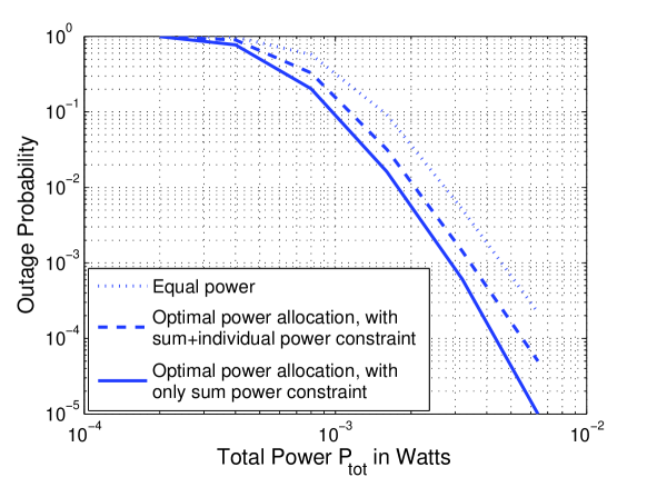
Figure 8: Effect of Individual Power Constraints (6 nodes)

IV-C Practical Issues

To obtain the desired transmit power levels for each sensor, we have assumed that the fusion center knows $\{(\gamma_{k},s_{k}):k=1,2,\ldots,K\}$. This assumption is reasonable in cases where the network condition and the signal being estimated change slowly in a quasi-static manner. We have also assumed that the fusion center executes the optimization and then appropriately activates the sensors with their respective power levels. Our approach is general for the estimation of a memoryless discrete-time random process $\theta(t)$. Due to the temporal memoryless property of the source and sensor observations, we can impose sample-by-sample estimation without significant estimation performance loss, but obtain important features such as easy implementation and minimum delay.

V Minimum-Power Estimation with Zero Outage

In the previous sections we have shown that with Rayleigh fading, non-zero outage is experienced when there are sum or individual power constraints. However, with $K$ observation sensors, it is possible to achieve order-$K$ estimation diversity for both equal-power and optimal power transmission strategies, while in the latter case we can further achieve certain adaptive power gain. In this section, we discuss a converse problem. Given a set of channel gains, which may be one realization of Rayleigh fading or may be simply caused by different transmission distances, we seek the optimal power allocation scheme to minimize the total power consumption while satisfying a certain distortion requirement. If the distortion requirement is satisfied with minimum power consumption for each given channel realization, we call such a scheme as minimum-power estimation with zero outage.

Based on the above discussion, the minimum-power estimation problem can be cast as

$$\min \sum_{k=1}^{K}P_{k}$$

s. t. $${\rm Var}[\hat{\theta}]\leq{D_{0}},$$

where $D_{0}$ is the distortion target. According to Eq. (1) and Eq. (4), given a set of channel SNR $[s_{1},s_{2},\cdots,s_{K}]$ and a set of local observation SNR $[\gamma_{1},\gamma_{2},\cdots,\gamma_{K}]$, the above problem is equivalent to

$$\min_{\alpha_{k}^{\prime}} \sum_{k=1}^{K}\alpha_{k}^{\prime}{(1+\gamma_{k}^{-1})}$$

s. t. $$\sigma_{\theta}^{2}\left(\sum_{k=1}^{K}\frac{{\alpha_{k}^{\prime}s_{k}}}{\gamma_{k}^{-1}{\alpha_{k}^{\prime}s_{k}}+1}\right)^{-1}\leq{D_{0}}$$

$$\alpha^{\prime}_{k}\geq 0,\hskip 8.5359ptk=1,\cdots,K$$

Unfortunately, this problem is not convex over the $\alpha_{k}^{\prime}$’s.

Let us define

$$r_{k}=\frac{{\alpha_{k}^{\prime}s_{k}}}{\gamma_{k}^{-1}{\alpha^{\prime}_{k}s_{k}}+1}=\frac{1}{\gamma_{k}^{-1}+\frac{1}{\alpha^{\prime}_{k}s_{k}}},\hskip 5.69046pt\forall k.$$ (20)

Then the above optimization problem is equivalent to

$$\min_{\alpha_{k}^{\prime},r_{k}} \sum_{k=1}^{K}\alpha^{\prime}_{k}{(1+\gamma_{k}^{-1})}$$

s. t. $$\sum_{k=1}^{K}r_{k}\geq\frac{\sigma_{\theta}^{2}}{D_{0}}$$

$$r_{k}=\frac{1}{\gamma_{k}^{-1}+\frac{1}{\alpha^{\prime}_{k}s_{k}}},\hskip 8.5359pt{\alpha^{\prime}_{k}}\geq 0,\hskip 8.5359pt\forall{k},$$

where we see that the variable $\alpha^{\prime}_{k}$ can be completely replaced by a function of $r_{k}$. From Eq. (20) we obtain that

$$\alpha^{\prime}_{k}=\frac{1}{s_{k}(r_{k}^{-1}-\gamma_{k}^{-1})},\hskip 5.69046pt\forall k.$$

Therefore, the problem can be transformed into a problem with variables $\{r_{1},r_{2},\dots,r_{K}\}$ shown as follows (noticing that $\eta_{k}:=s_{k}/(1+\gamma_{k}^{-1})$):

$$\min_{r_{k}} \sum_{k=1}^{K}\frac{1+\gamma_{k}^{-1}}{s_{k}(r_{k}^{-1}-\gamma_{k}^{-1})}=\sum_{k=1}^{K}\frac{\eta_{k}^{-1}}{r_{k}^{-1}-\gamma_{k}^{-1}}$$

s. t. $$\sum_{k=1}^{K}r_{k}\geq\frac{\sigma_{\theta}^{2}}{D_{0}};\hskip 8.5359pt0\leq{r_{k}}<\gamma_{k},\hskip 8.5359pt\forall{k}$$ (21)

which is convex over $r_{k}$. The upper limit on $r_{k}$ in the second constraint is due to the fact that $r_{k}=\frac{1}{\gamma_{k}^{-1}+\frac{1}{\alpha^{\prime}_{k}s_{k}}}$ and $\frac{1}{\alpha^{\prime}_{k}s_{k}}\geq 0$.

Similar to solving Eq. (IV-A) in Section IV, the solution of Eq. (V) can be stated as follows. As before, we rank the sensors according to $\eta_{1}\geq\eta_{2}\geq\ldots\geq\eta_{K}$, and define

$$g(k)=1-\frac{D(k)}{\sqrt{\eta_{k}}C(k)},\quad\mbox{for\ }1\leq{k}\leq{K},$$ (22)

where $C(k)=\displaystyle\sum_{m=1}^{k}\frac{\gamma_{m}}{\sqrt{\eta_{m}}}$ and $D(k)=\displaystyle\sum_{m=1}^{k}\gamma_{m}-\frac{\sigma_{\theta}^{2}}{D_{0}}$. Find $K_{1}$ such that $g(K_{1})>0$ and $g(K_{1}+1)\leq 0$. If $g(k)>0$ for all $1\leq k\leq K$, we take $K_{1}=K$. Also define $\rho_{0}={C(K_{1})}/{D(K_{1})}$. Then the optimal solution is given as

$$r_{k}^{opt}=\gamma_{k}\left(1-\sqrt{\eta_{k}^{-1}}\rho_{0}\right)^{+},\hskip 8.5359pt\forall\ {k}$$ (23)

where $(x)^{+}$ equals $0$ when $x<0$, and otherwise equals $x$.

Hence, by definition, we have

$${\alpha^{\prime}_{k}}^{opt} = \frac{1}{s_{k}\left((r_{k}^{opt})^{-1}-\gamma_{k}^{-1}\right)}$$ (26)

$$= \left\{\begin{array}[]{ll}0,&k>K_{1}\\ \displaystyle\frac{\gamma_{k}}{s_{k}}\left(\sqrt{\eta_{k}^{-1}}\rho_{0}-1\right),&k\leq K_{1}.\end{array}\right.$$

Similar to the result in Section IV, we see that the optimal strategy for minimum-power transmission with zero outage is to only allocate transmit power to sensors with better channel SNR and observation quality. Again, the figure of merit is $\eta_{k}={s_{k}}/{(1+\gamma_{k}^{-1})}$. If a sensor has a $\eta_{k}$ below certain threshold, it should be turned off to save power. Also not surprisingly, the solution in Eq. (26) is very similar to the one in Eq. (15) except that the universal constants $c_{0}$ and $\rho_{0}$ are different. In Eq. (15), $c_{0}$ is determined by the power constraint, while in Eq. (26) $\rho_{0}$ is determined by the distortion requirement..

We now solve the optimization problem to show how much power we can save compared with an equal-power transmission strategy that satisfies the zero-outage distortion requirement with minimum sum power. We use the same setup as Section III except that we now have $100$ sensors and draw the average sum power consumption over different distortion target values. At each distortion target $D_{0}$, the required sum power is averaged over $10,000$ independent channel realizations. The result is shown in Fig. 9, where we see that the more strict distortion requirement we have (smaller $D_{0}$), the more power we can save by deploying the optimal power allocation strategies, which is very important in energy-constrained sensor networks.

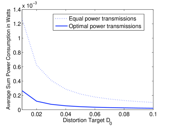
Figure 9: Average sum power vs. distortion requirements

Discussion of Maximizing Sensor Network Lifetime

In our model we minimize the power sum $\sum_{k}{P_{k}}$, i.e., the $L^{1}$-norm of the transmission power vector $\mathbf{P}=[P_{1},P_{2},\ldots,P_{K}]$. If the channel gain and the variance of the observation noise for each sensor are ergodically time-varying on a block-by-block basis, minimizing the $L^{1}$-norm of $\mathbf{P}$ in each time block minimizes $E\{\sum_{k}{P_{k}}\}$. In other words, it maximizes the lower bound of the average node lifetime that is defined as $\frac{1}{K}\sum_{k}\frac{E_{0}}{E\{P_{k}\}}$ with $E_{0}$ the battery energy available to each sensor (we assume that $E_{0}$ is the same for all the sensors). This can be proved from the fact that

$$\frac{1}{K}\sum_{k}\frac{E_{0}}{E\{P_{k}\}}\geq\frac{E_{0}}{E\{\frac{1}{K}\sum_{k}{P_{k}}\}},$$

which is based on Jensen’s inequality [29]. However, when the channel is static and the variance of the observation noise is time-invariant, minimizing the $L^{1}$-norm may lead some individual sensors to consume too much power and die out quickly. In this case minimizing the $L^{\infty}$-norm, i.e., minimizing the maximum of the individual power values, is the fairest for all sensors, but the total power consumption can be high. A good compromise is to minimize the $L^{2}$-norm of $\mathbf{P}$ [30]. In this way, we can penalize the large terms in the power vector while still keeping the total power consumption reasonably low. Specifically, for the $L^{2}$-norm minimization, the problem formulation becomes

$$\min_{r_{k}} \sum_{k=1}^{K}\left(\frac{\eta_{k}^{-1}}{r_{k}^{-1}-\gamma_{k}^{-1}}\right)^{2}$$

s. t. $$\sum_{k=1}^{K}r_{k}\geq\frac{\sigma_{\theta}^{2}}{D_{0}};\hskip 8.5359pt0\leq{r_{k}}<\gamma_{k},\hskip 8.5359pt\forall{k}$$ (27)

which is still a convex problem. Note that minimizing the various norms of $\mathbf{P}$ may not be the optimal thing to do given the fact that we are still lack of a unified definition of sensor network lifetime. A complete description of this problem is beyond the scope of this paper.

VI Conclusions

For the distributed estimation of an unknown source, we have introduced a new concept of estimation outage and defined the corresponding estimation diversity, for the case of i.i.d. observation noise variances at different sensors and i.i.d. fading channels between the sensors and the fusion center. We have shown that the full estimation diversity (on the order of the number of sensor nodes $K$) can be achieved even with simple equal-power transmission strategies. We have further shown that the end-to-end distortion can be minimized under sum power constraints, where we gain certain adaptive power gain on top of the full diversity gain by turning off sensors with bad channels and bad observation quality. Moreover, we demonstrated that by considering an extra individual power constraint at each sensor, certain performance loss occurs. Minimum-power transmission with zero estimation outage has also been investigated, where significant power savings is achieved over equal-power transmission schemes.

appendix

VI-A Derivation of $D_{\infty}$ in Eq. (6)

We start with

$$\frac{{P_{tot}s_{k}}}{K(1+\gamma_{k}^{-1})}-\frac{{P_{tot}s_{k}}}{\gamma_{k}^{-1}{P_{tot}s_{k}}+K(1+\gamma_{k}^{-1})}$$

$$= \frac{\gamma_{k}^{-1}{P_{tot}^{2}s_{k}^{2}}}{K(1+\gamma_{k}^{-1})\left(\gamma_{k}^{-1}{P_{tot}s_{k}}+K(1+\gamma_{k}^{-1})\right)}$$

$$\leq \frac{\gamma_{k}^{-1}{P_{tot}^{2}s_{k}^{2}}}{K^{2}}.$$

Thus we have the following inequalities:

$$\frac{{P_{tot}s_{k}}}{K(1+\gamma_{k}^{-1})}-\frac{\gamma_{k}^{-1}{P_{tot}^{2}s_{k}^{2}}}{K^{2}}$$

$$\leq \frac{{P_{tot}s_{k}}}{\gamma_{k}^{-1}{P_{tot}s_{k}}+K(1+\gamma_{k}^{-1})}$$

$$\leq \frac{{P_{tot}s_{k}}}{K(1+\gamma_{k}^{-1})}.$$

Therefore, according to Eq. (5), we have

$$\sum_{k=1}^{K}\frac{{P_{tot}s_{k}}}{K(1+\gamma_{k}^{-1})}-\sum_{k=1}^{K}\frac{\gamma_{k}^{-1}{P_{tot}^{2}s_{k}^{2}}}{K^{2}}$$ (28)

$$\leq \sigma_{\theta}^{2}\left({\rm Var}[\hat{\theta}]\right)^{-1}$$

$$\leq \sum_{k=1}^{K}\frac{{P_{tot}s_{k}}}{K(1+\gamma_{k}^{-1})}.$$

It follows from the strong Law of Large Numbers (LLN) [27] that when $K\to\infty$,

$$\sum_{k=1}^{K}\frac{{P_{tot}s_{k}}}{K(1+\gamma_{k}^{-1})}\to P_{tot}E[s_{1}/(1+\gamma_{1}^{-1})],$$

$$\quad\sum_{k=1}^{K}\frac{\gamma_{k}^{-1}{P_{tot}^{2}s_{k}^{2}}}{K}\to P_{tot}^{2}E\left(\gamma_{1}^{-1}{s_{1}^{2}}\right),$$

$$\quad{\rm and}\quad\sum_{k=1}^{K}\frac{\gamma_{k}^{-1}{P_{tot}^{2}s_{k}^{2}}}{K^{2}}\to 0,$$

providing that $E[s_{k}/(1+\gamma_{k})]$ and $E[\gamma_{k}^{-1}{s_{k}^{2}}]$ are finite. Therefore,

$$\lim_{K\rightarrow\infty}\sigma_{\theta}^{2}\left({\rm Var}[\hat{\theta}]\right)^{-1}=P_{tot}E[s_{1}/(1+\gamma_{1}^{-1})],$$ (29)

which implies that

$$\lim_{K\rightarrow\infty}{\rm Var}[\hat{\theta}]=\frac{\sigma_{\theta}^{2}}{P_{tot}E[s_{1}/(1+\gamma_{1}^{-1})]}:=D_{\infty}.$$ (30)

VI-B Proof of Theorem III.1

Based on the result from the large deviation theory [27], we first establish the following lemma.

Lemma VI.1

Suppose $\beta_{k}:k=1,\ldots,K$ are i.i.d. random variables, and $a$ is a constant satisfying $a<E(\beta_{k})$. Then for any $K\geq 1$,

$${\rm Prob}\left\{\frac{1}{K}\sum_{k=1}^{K}\beta_{k}<a\right\}\leq\exp(-KI_{\beta}(a)),$$ (31)

where $I_{\beta}(a)$ is the rate function of $\beta_{k}$ which is defined to be

$$I_{\beta}(a)=\sup_{\theta\in\mathbb{R}}(\theta a-\log M_{\beta}(\theta)),$$ (32)

and $M_{\beta}(\theta)$ is the moment generating function of $\beta_{k}$. Similarly, if $a>E(\beta_{k})$, then for any $K\geq 1$,

$${\rm Prob}\left\{\frac{1}{K}\sum_{k=1}^{K}\beta_{k}>a\right\}\leq\exp(-KI_{\beta}(a)).$$

Remark VI.2

The exponent $I_{\beta}(a)$ in Eq. (32) is nonnegative (since $I_{\beta}(a)\geq\left(\theta a-\log M_{\beta}(\theta)\right)|_{\theta=0}=0$) and convex over $a$ (since it is the supremum of linear functions, and is hence convex). Also it holds that $I_{\beta}(a)=0$ if $a=E(\beta_{k})$, $I_{\beta}(a)$ is an increasing function of $a$ for $a\geq E(\beta_{k})$, and is an decreasing function of $a$ for $a\leq E(\beta_{k})$. In addition, $I_{\beta}(a)$ leads to a tight bound in Eq. (31) in the sense that

$$\lim_{K\to\infty}-\frac{1}{K}\log\left({\rm Prob}\left\{\frac{1}{K}\sum_{k=1}^{K}\beta_{k}<a\right\}\right)=I_{\beta}(a)$$ (33)

if i) $M_{\beta}(\theta)$ is finite in some neighborhood of $\theta=0$ and ii) $M_{\beta}(\theta)$ is differentiable in a neighborhood of $\theta^{*}$ where the supremum in Eq. (32) is reached at $\theta^{*}$. More details can be found in [27] or Section III of [28].

We now continue to prove Theorem III.1. From the second inequality in Eq. (28), we get

$${\mathcal{P}_{D_{0}}} = {\rm Prob}\left\{{\rm Var}[\hat{\theta}]>D_{0}\right\}$$

$$\geq {\rm Prob}\left\{\sum_{k=1}^{K}\frac{P_{tot}s_{k}}{K(1+\gamma_{k}^{-1})}<\frac{\sigma_{\theta}^{2}}{D_{0}}\right\}$$

$$= {\rm Prob}\left\{\frac{1}{K}\sum_{k=1}^{K}\frac{s_{k}}{1+\gamma_{k}^{-1}}<\frac{\sigma_{\theta}^{2}}{D_{0}P_{tot}}\right\}$$

$$= {\rm Prob}\left\{\frac{1}{K}\sum_{k=1}^{K}\frac{s_{k}}{1+\gamma_{k}^{-1}}<a\right\},$$

where we introduce the constant $a=\sigma_{\theta}^{2}/(D_{0}P_{tot})$. This implies that

$$\lim_{K\to\infty}-\frac{1}{K}\log{\mathcal{P}_{D_{0}}}$$

$$\leq \lim_{K\to\infty}-\frac{1}{K}\log\left({\rm Prob}\left\{\frac{1}{K}\sum_{k=1}^{K}\frac{s_{k}}{1+\gamma_{k}^{-1}}<a\right\}\right).$$

On the other hand, from the first inequality in Eq. (28) we obtain

$$\lim_{K\to\infty}-\frac{1}{K}\log{\mathcal{P}_{D_{0}}}$$

$$= \lim_{K\to\infty}-\frac{1}{K}\log\left({\rm Prob}\left\{{\rm Var}[\hat{\theta}]>D_{0}\right\}\right)$$

$$\geq \lim_{K\to\infty}-\frac{1}{K}\log\left({\rm Prob}\left\{\sum_{k=1}^{K}\frac{{P_{tot}s_{k}}}{K(1+\gamma_{k}^{-1})}\right.\right.$$

$$\left.\left.-\sum_{k=1}^{K}\frac{\gamma_{k}^{-1}{P_{tot}^{2}s_{k}^{2}}}{K^{2}}<\frac{\sigma_{\theta}^{2}}{D_{0}}\right\}\right)$$

$$\;{\buildrel{\rm(a)}\over{=}}\; \lim_{K\to\infty}-\frac{1}{K}\log\left({\rm Prob}\left\{\sum_{k=1}^{K}\frac{{P_{tot}s_{k}}}{K(1+\gamma_{k}^{-1})}<\frac{\sigma_{\theta}^{2}}{D_{0}}\right\}\right)$$

$$= \lim_{K\to\infty}-\frac{1}{K}\log\left({\rm Prob}\left\{\frac{1}{K}\sum_{k=1}^{K}\frac{s_{k}}{1+\gamma_{k}^{-1}}<a\right\}\right).$$

where $(a)$ is due to the following lemma.

Lemma VI.3

Suppose $\{\nu_{k}:1\leq k\leq K\}$, $\{\beta_{k}:1\leq k\leq K\}$ are two sets of i.i.d. random variables with bounded first moments, $c_{1}$ is a constant satisfying $c_{1}<E(\nu_{k})$, and $E(\beta_{k})=b$. Further assume that $\nu_{k}$ and $\beta_{k}$ both satisfy the regularity requirements described in Remark VI.2, then

$$\lim_{K\to\infty}-\frac{1}{K}\log\left({\rm Prob}\left\{\frac{1}{K}\sum_{k=1}^{K}\nu_{k}-\frac{1}{K^{2}}\sum_{k=1}^{K}\beta_{k}<c_{1}\right\}\right)$$ (34)

$$= \lim_{K\to\infty}-\frac{1}{K}\log\left({\rm Prob}\left\{\frac{1}{K}\sum_{k=1}^{K}\nu_{k}<c_{1}\right\}\right).$$

Proof:

We prove $A=B$ by proving $A\geq{B}$ and $A\leq{B}$ hold at the same time. First it is obvious that “$\leq$” holds in Eq. (34) since

$${\rm Prob}\left\{\frac{1}{K}\sum_{k=1}^{K}\nu_{k}-\frac{1}{K^{2}}\sum_{k=1}^{K}\beta_{k}<c_{1}\right\}$$

$$\geq{\rm Prob}\left\{\frac{1}{K}\sum_{k=1}^{K}\nu_{k}<c_{1}\right\}.$$

We next show the inequality of the other direction. For any $K\in\mathbb{Z}^{+}$ and $\epsilon>0$, it holds that

$${\rm Prob}\left\{\frac{1}{K}\sum_{k=1}^{K}\nu_{k}-\frac{1}{K^{2}}\sum_{k=1}^{K}\beta_{k}<c_{1}\right\}$$

$$= {\rm Prob}\left\{\frac{1}{K}\sum_{k=1}^{K}\nu_{k}-\frac{1}{K^{2}}\sum_{k=1}^{K}\beta_{k}<c_{1},\;\frac{1}{K^{2}}\sum_{k=1}^{K}\beta_{k}\leq\epsilon\right\}$$

$$+{\rm Prob}\left\{\frac{1}{K}\sum_{k=1}^{K}\nu_{k}-\frac{1}{K^{2}}\sum_{k=1}^{K}\beta_{k}<c_{1},\;\frac{1}{K^{2}}\sum_{k=1}^{K}\beta_{k}>\epsilon\right\}$$

$$\leq {\rm Prob}\left\{\frac{1}{K}\sum_{k=1}^{K}\nu_{k}<c_{1}+\epsilon\right\}+{\rm Prob}\left\{\frac{1}{K^{2}}\sum_{k=1}^{K}\beta_{k}>\epsilon\right\}.$$

Taking $\epsilon=b/\sqrt{K}$, we obtain

$${\rm Prob}\left\{\frac{1}{K}\sum_{k=1}^{K}\nu_{k}-\frac{1}{K^{2}}\sum_{k=1}^{K}\beta_{k}<c_{1}\right\}$$ (35)

$$\leq {\rm Prob}\left\{\frac{1}{K}\sum_{k=1}^{K}\nu_{k}<c_{1}+\frac{b}{\sqrt{K}}\right\}$$

$$+{\rm Prob}\left\{\frac{1}{K}\sum_{k=1}^{K}\beta_{k}>\sqrt{K}b\right\}.$$

Lemma VI.1 implies that

$$\lim_{K\to\infty}-\frac{1}{K}\log\left({\rm Prob}\left\{\frac{1}{K}\sum_{k=1}^{K}\nu_{k}<c_{1}+\frac{b}{\sqrt{K}}\right\}\right)$$ (36)

$$= \lim_{K\to\infty}I_{a}(c_{1}+\frac{b}{\sqrt{K}})$$

$$= I_{a}(c_{1}),$$

where $I_{a}$ is the rate function of $\nu_{k}$. Also

$$\lim_{K\to\infty}-\frac{1}{K}\log\left({\rm Prob}\left\{\frac{1}{K}\sum_{k=1}^{K}\beta_{k}>\sqrt{K}b\right\}\right)$$ (37)

$$= \lim_{c_{2}\to\infty}I_{b}(c_{2})$$

$$= +\infty,$$

where $I_{b}$ is the rate function of $\beta_{k}$.

Therefore, it follows from Eqns (35)–(37) that

$$\!\!\!\!\!\!\!\!\!\!\!\!\lim_{K\to\infty}-\frac{1}{K}\log\left({\rm Prob}\left\{\frac{1}{K}\sum_{k=1}^{K}\nu_{k}-\frac{1}{K^{2}}\sum_{k=1}^{K}\beta_{k}<c_{1}\right\}\right)$$

$$\geq I_{a}(c_{1})$$

$$= \lim_{K\to\infty}-\frac{1}{K}\log\left({\rm Prob}\left\{\frac{1}{K}\sum_{k=1}^{K}\nu_{k}<c_{1}\right\}\right).$$

The proof of the lemma is thus completed. ∎

In summary, we have

$$\lim_{K\to\infty}-\frac{1}{K}\log{\mathcal{P}_{D_{0}}}$$

$$= \lim_{K\to\infty}-\frac{1}{K}\log\left({\rm Prob}\left\{\frac{1}{K}\sum_{k=1}^{K}\frac{s_{k}}{1+\gamma_{k}^{-1}}<a\right\}\right).$$

Since $s_{k}/(1+\gamma_{k}^{-1})$ are i.i.d. random variables, we can apply Lemma VI.1 to calculate the rate function.

Applying Lemma VI.1 and assuming that the mild regularity conditions for $M(\theta)$ described in the above remark hold, we obtain Theorem III.1.

Shuguang Cui (S’99–M’05) received Ph.D in Electrical Engineering from Stanford University, California, USA, M.Eng in Electrical Engineering from McMaster University, Hamilton, Canada, in 2000, and B.Eng. in Radio Engineering with the highest distinction from Beijing University of Posts and Telecommunications, Beijing, China, in 1997. He is now working as an assistant professor in Electrical and Computer Engineering at the University of Arizona, Tucson, AZ. From 1997 to 1998 he worked at Hewlett-Packard, Beijing, P. R. China, as a system engineer. In the summer of 2003, he worked at National Semiconductor, Santa Clara, CA, on the ZigBee project. His current research interests include cross-layer energy minimization for low-power sensor networks, hardware and system synergies for high-performance wireless radios, statistical signal processing, and general communication theories. He was a recipient of the NSERC graduate fellowship from the National Science and Engineering Research Council of Canada and the Canadian Wireless Telecommunications Association (CWTA) graduate scholarship.

Jin-Jun Xiao (S’04–M’07) received the B.Sc. degree in Applied Mathematics from Jilin University, Changchun, China, in 1997, and the M.Sc. degree in Mathematics and Ph.D. degree in Electrical Engineering from the University of Minnesota, Twin Cities, in 2003 and 2006 respectively. He is currently a Postdoctoral Fellow at the Washington University in St. Louis, Missouri. In the summer of 2002, Dr. Xiao worked on barcode signal processing at Symbol Technologies, Holtsville, New York. His current research interests are in distributed signal processing, multiuser information theory and their application to wireless sensor networks.

Andrea J. Goldsmith (S’90–M’93–SM’99–F’05) is a professor of Electrical Engineering at Stanford University, and was previously an assistant professor of Electrical Engineering at Caltech. She has also held industry positions at Maxim Technologies and at AT$\&$T Bell Laboratories, and is currently on leave from Stanford as co-founder and CTO of a wireless startup company. Her research includes work on capacity of wireless channels and networks, wireless communication theory, energy-constrained wireless communications, wireless communications for distributed control, and cross-layer design of wireless networks. She is author of the book “Wireless Communications” and co-author of the book “MIMO Wireless Communications,” both published by Cambridge University Press. She received the B.S., M.S. and Ph.D. degrees in Electrical Engineering from U.C. Berkeley. Dr. Goldsmith is a Fellow of the IEEE and of Stanford, and currently holds Stanford’s Bredt Faculty Development Scholar Chair. She has received several awards for her research, including the National Academy of Engineering Gilbreth Lectureship, the Alfred P. Sloan Fellowship, the Stanford Terman Fellowship, the National Science Foundation CAREER Development Award, and the Office of Naval Research Young Investigator Award. She was also a co-recipient of the 2005 IEEE Communications Society and Information Theory Society joint paper award. She currently serves as associate editor for the IEEE Transactions on Information Theory and as editor for the Journal on Foundations and Trends in Communications and Information Theory and in Networks. She was previously an editor for the IEEE Transactions on Communications and for the IEEE Wireless Communications Magazine, and has served as guest editor for several IEEE journal and magazine special issues. Dr. Goldsmith is active in committees and conference organization for the IEEE Information Theory and Communications Societies, and is currently serving as technical program co-chair for ISIT 2007. She is an elected member of the Board of Governers for both societies, a distinguished lecturer for the IEEE Communications Society, and the second vice-president and student committee chair of the IEEE Information Theory Society.

Zhi-Quan (Tom) Luo (F’07) received his B.Sc. degree in Applied Mathematics in 1984 from Peking University, Beijing, China. Subsequently, he was selected by a joint committee of American Mathematical Society and the Society of Industrial and Applied Mathematics to pursue Ph.D study in the United States. After an one-year intensive training in mathematics and English at the Nankai Institute of Mathematics, Tianjin, China, he entered the Operations Research Center and the Department of Electrical Engineering and Computer Science at MIT, where he received a Ph.D degree in Operations Research in 1989. From 1989 to 2003, Dr. Luo held a faculty position with the Department of Electrical and Computer Engineering, McMaster University, Hamilton, Canada, where he eventually became the department head and held a Canada Research Chair in Information Processing. Since April of 2003, he has been with the Department of Electrical and Computer Engineering at the University of Minnesota (Twin Cities) as a full professor and holds an endowed ADC Chair in digital technology. His research interests lie in the union of optimization algorithms, data communication and signal processing. Prof. Luo serves on the IEEE Signal Processing Society Technical Committees on Signal Processing Theory and Methods (SPTM), and on the Signal Processing for Communications (SPCOM). He is a co-reciept of the 2004 IEEE Signal Processing Society’s Best Paper Award, and has held editorial positions for several international journals including Journal of Optimization Theory and Applications, Mathematics of Computation, and IEEE Transactions on Signal Processing. He currently serves on the editorial boards for a number of international journals including SIAM Journal on Optimization, Mathemtical Programming, and Mathematics of Operations Research.

H. Vincent Poor (S’72–M’77–SM’82–F’87) received the Ph.D. degree in EECS from Princeton University in 1977. From 1977 until 1990, he was on the faculty of the University of Illinois at Urbana-Champaign. Since 1990 he has been on the faculty at Princeton, where he is the Dean of Engineering and Applied Science, and the Michael Henry Strater University Professor of Electrical Engineering. Dr. Poor’s research interests are in the areas of stochastic analysis, statistical signal processing, and their applications in wireless networks and related fields. Among his publications in these areas is the recent book MIMO Wireless Communications (Cambridge University Press, 2007). Dr. Poor is a member of the National Academy of Engineering and is a Fellow of the American Academy of Arts and Sciences. He is also a Fellow of the Institute of Mathematical Statistics, the Optical Society of America, and other organizations. In 1990, he served as President of the IEEE Information Theory Society, and he is currently serving as the Editor-in-Chief of the IEEE Transaction on Information Theory. Recent recognition of his work includes a Guggenheim Fellowship and the IEEE Education Medal.

References

- [1] D. A. Castanon and D. Teneketzis, “Distributed estimation algorithms for nonlinear systems,” IEEE Transactions on Automatic Control, vol. 30, no. 5, pp. 418-425, May 1985.
- [2] H. C. Papadopoulos, G.W. Wornell, and A. V. Oppenheim, “Sequential signal encoding from noisy measurements using quantizers with dynamic bias control,” IEEE Trans. Inform. Theory, vol. 47, no. 3, pp. 978-1002, Mar. 2001.
- [3] A. S. Willsky, M. Bello, D. A. Castanon, B. C. Levy, and G. Verghese, “Combining and updating of local estimates and regional maps along sets of one-dimensional tracks,” IEEE Transactions on Automatic Control, vol. 27, no. 4, pp. 799-813, Aug. 1982.
- [4] J. A. Gubner, “Distributed estimation and quantization,” IEEE Trans. Inform. Theory, vol. 39, no. 4, pp. 1456-1459, Jul. 1993.
- [5] Z.-Q. Luo and J. N. Tsitsiklis, “Data fusion with minimal communication,” IEEE Trans. Inform. Theory, vol. 40, no. 5, pp. 1551-1563, Sep. 1994.
- [6] M. Gastpar and M. Vetterli, “Source-channel communication in sensor networks,” Lecture Notes in Computer Science, vol. 2634, pp. 162-177, Springer, New York, Apr. 2003.
- [7] A. D. Sarwate and M. Gastpar, “Fading observation alignment via feedback,” Proc. the Fourth International Symposium on Information Processing in Sensor Networks, 2005.
- [8] K. Eswaran and M. Gastpar, “On the quadratic AWGN CEO problem and non-Gaussian sources,” Proc. IEEE Int Symp Info Theory, pp. 219-223, Adelaide, Australia, Sep. 2005.
- [9] K. Liu, H. El-Gamal, and A. Sayeed, “On optimal parametric field estimation in sensor networks,” Proc. IEEE/SP 13th Workshop on Statistical Signal Processing, pp. 1170-1175, Jul. 2005.
- [10] W. Bajwa, A. Sayeed, and R. Nowak, “Matched source-channel communication for field estimation in wireless sensor network,” Proc. the Fouth Int. Symposium on Information Processing in Sensor Networks, 2005.
- [11] G. Mergen and L. Tong, “Type based estimation over multiaccess channels,” IEEE Transactions on Signal Processing, vol. 54, no. 2, pp. 613-626, Feb. 2006.
- [12] K. Liu and A. Sayeed, “Optimal distributed detection strategies for wireless sensor networks,” The 43rd Allerton Conference on Communication, Control, and Computing, Monticello, IL, Oct. 2004.
- [13] D. Marco, E. Duarte-Melo, M. Liu, and D. Neuhoff, “On the many-to-one transport capacity of a dense wireless sensor network and the compressibility of its data,” Proc. the Second Int. Symposium on Information Processing in Sensor Networks, 2003.
- [14] P. Ishwar, R. Puri, K. Ramchandran, and S. S. Pradhan, “On rate-constrained distributed estimation in unreliable sensor networks,” IEEE Journal on Selected Areas in Communications, vol. 23, no. 4, pp. 765-775, Apr. 2005.
- [15] R. Nowak, U. Mitra, and R. Willet, “Estimating inhomogeneous fields using wireless sensor networks,” IEEE J. Selected Areas in Comm, vol. 22, no. 6, pp. 999-1006, Aug. 2004.
- [16] L. Xiao, S. Boyd, and S. Lall, “A scheme for robust distributed sensor fusion based on average consensus,” Proc. tthe Fouth Int. Symposium on Information Processing in Sensor Networks, 2005.
- [17] Z.-Q. Luo, “Universal Decentralized Estimation in a Bandwidth Constrained Sensor Network,” IEEE Trans. Inform. Theory, vol. 51, no. 6, pp. 2210-2219, Jun. 2005.
- [18] J.-J. Xiao and Z.-Q. Luo, “Universal decentralized estimation in an inhomogeneous sensing environment,” IEEE Trans. Inform. Theory, vol. 51, no. 10, pp. 3564-3575, Oct. 2005.
- [19] T. J. Goblick, “Theoretical limitations on the transmission of data from analog sources,” IEEE Trans. Inform. Theory, vol. 11, pp. 558-567, Oct. 1965.
- [20] M. Gastpar, B. Rimoldi, and M. Vetterli, “To code, or not to code: lossy source-channel communication revisited,” IEEE Trans. Inform. Theory, vol. 49 pp. 1147-1158, May 2003.
- [21] J. M. Mendel, Lessons in Estimation Theory for Signal Processing, Communications, and Control, Prentice Hall, Englewood Cliffs, NJ, 1995.
- [22] A. D’Costa, V. Ramchandran, and A. Sayeed, “Distributed classification of gaussian space-time sources in wireless sensor networks,” IEEE J. Selected Areas in Comm, vol. 22, no. 6, pp. 1026-1036, Aug. 2004.
- [23] J. F. Chamberland and V. Veeravalli, “Asymptotic results for decentralized detection in power-constrained wireless sensor networks,” IEEE J. Selected Areas in Comm, vol. 22, no. 6, pp. 1007-1015, Aug. 2004.
- [24] J.-J. Xiao and Z.-Q. Luo, “Universal decentralized detection in a bandwidth constrained sensor network,” IEEE Transations on Signal Processing, vol. 53, no. 8, pp. 2617-2624, Aug. 2005.
- [25] J.-J. Xiao, Z.-Q. Luo, S. Cui, and A. J. Goldsmith, “Power-efficient analog forwarding transmission in an inhomogeneous Gaussian sensor network,” IEEE Workshop on Signal Processing Advances in Wireless Communications, pp. 121-125, New York, NY, Jun. 2005.
- [26] J.-J. Xiao, S. Cui, Z.-Q. Luo, and A.J. Goldsmith, “Linear coherent decentralized estimation,” to appear at IEEE Globecom, San Francisco, CA, Nov. 2006. Available at: http://www.ece.umn.edu/users/xiao/.
- [27] A. Dembo and O. Zeitouni, Large Deviations Techniques and Applications, Jones and Bartlett, Boston, 1993.
- [28] A. Weiss, “An introduction to large deviations for communication networks”, IEEE J. Selected Areas in Comm, Vol. 13, no. 6, pp. 938-952, Aug. 1995.
- [29] S. Boyd and L. Vandenberghe, Convex Optimization, Cambridge Univ. Press, Cambridge, U.K., 2003.
- [30] J.-J. Xiao, S. Cui, Z.-Q. Luo, and A. J. Goldsmith, “Power scheduling of universal decentralized estimation in sensor networks,” IEEE Transactions on Signal Processing, vol. 54, no. 2, pp. 413-422, Feb. 2006.
- [31] A. Paulraj, R. Nabar, and D. Gore, Introduction to Space-Time Wireless Communications, Cambridge University Press, Cambridge, UK, 2003.