Radial density profiles of time-delay lensing galaxies

Abstract

We present non-parametric radial mass profiles for ten QSO strong lensing galaxies. Five of the galaxies have profiles close to $\rho(r)\propto r^{-2}$, while the rest are closer to $r^{-1}$, consistent with an NFW profile. The former are all relatively isolated early-types and dominated by their stellar light. The latter —though the modeling code did not know this— are either in clusters, or have very high mass-to-light, suggesting dark-matter dominant lenses (one is a actually pair of merging galaxies). The same models give $H_{0}^{-1}=15.2_{-1.7}^{+2.5}\,{\rm Gyr}$ ($H_{0}=64_{-9}^{+8}\,{\rm km\,s^{-1}\,Mpc^{-1}}$), consistent with a previous determination. When tested on simulated lenses taken from a cosmological hydrodynamical simulation, our modeling pipeline recovers both $H_{0}$ and $\rho(r)$ within estimated uncertainties.

Our result is contrary to some recent claims that lensing time delays imply either a low $H_{0}$ or galaxy profiles much steeper than $r^{-2}$. We diagnose these claims as resulting from an invalid modeling approximation: that small deviations from a power-law profile have a small effect on lensing time-delays. In fact, as we show using using both perturbation theory and numerical computation from a galaxy-formation simulation, a first-order perturbation of an isothermal lens can produce a zeroth-order change in the time delays.

1 Introduction

In our current understanding of structure formation, galaxies form from the dissipation of gas within dark matter halos (see e.g., White & Rees, 1978). Cosmological simulations suggest that these halos are self-similar, with universal density profiles (see e.g., Navarro et al., 1996; Diemand et al., 2004; Hayashi et al., 2004; Merritt et al., 2006; Graham et al., 2006a, b; Moore et al., 1998). The dark-matter halos are commonly fit to the well-known NFW profile

$$\rho\propto\frac{1}{(r/a)^{\alpha}(1+r/a)^{3-\alpha}}$$ (1)

with $\alpha$ is numerically found to be in the range $\alpha\sim[1,1.5]$, but other parameterizations are also possible (e.g., Merritt et al., 2006; Graham et al., 2006a, b). Over the visible region of galaxies ($r\ll a$), the dark matter distribution tends towards a single power law with: $\rho\sim r^{-\alpha}$. At much larger radii ($r\gg a$), the distribution tends towards $\rho\sim r^{-3}$.

While the distribution of dark matter is now relatively well understood, less clear is the effect of the gaseous component on the final total mass distribution of galaxies, since simulations involving gas remain a significant technical challenge (see e.g., Mayer, 2004). However, it is likely to be more complex than a simple sum of the gaseous, stellar and dark matter components, since the gas collapse will cause a contraction of the underlying dark matter distribution, increasing the central concentration of dark matter, and possibly even making the halo more spherical (e.g., Young, 1980; Kazantzidis et al., 2004). Despite these worries, the final resulting mass distribution is simpler to predict if the stars and gas form the dominant dynamical component of the galaxy – as is the case in the centre of massive spiral galaxies and ellipticals. There we may expect an isothermal distribution ($\rho\propto r^{-2}$), either as a result of equilibrium gas physics (Shu, 1991), or relaxation (Lynden-Bell, 1967). Indeed, dynamical measurements of massive galaxies suggest that an isothermal distribution provides an excellent fit over a wide range of radii (see e.g., van der Marel, 1991; Kronawitter et al., 2000; Humphrey et al., 2006). At larger radii, however, we expect a transition from $\rho\sim r^{-2}$ to $\rho\sim r^{-1}$ as the dark matter halo becomes more and more dynamically dominant. Eventually, at very large radii ($r\gg a$) we expect a second transition to $\rho\sim r^{-3}$.

In this paper, we test the above theoretical predictions by using strong lensing to determine the non-parametric density profile of ten QSO lensing galaxies, for the first time. Strong lensing measurements, which are limited in radius to the outermost observed image, probe radii $r<a$. Thus, we hope to probe the transition from $\rho\sim r^{-2}$ to $\rho\sim r^{-1}$ as we move from galaxies dynamically dominated by their stars, to galaxies dynamically dominated by their dark matter. We do not measure far enough out ($r>a$) to test the prediction of an eventual transition to $\rho\sim r^{-3}$.

2 The method

2.1 Searching lens models

A given set of lensing observables, even with zero noise, is consistent with a variety of lensing mass distributions. This is the well-known problem of lensing degeneracies. If multiple source redshifts are available, as is the case in rich lensing clusters, the effect of degeneracies is minimal, enabling robust mapping of the mass profiles (Saha et al., 2006c). For galaxy lenses, however, multiple source redshifts are very unlikely, and as a result degeneracies present a serious difficulty. The most important degeneracy couples time delays and the steepness of the mass profile: steeper mass profiles have higher values of $(H_{0}\,\Delta t)$ for the same image positions and magnification ratios.

Given the steepness degeneracy, one might hope that if $\Delta t$ and $H_{0}$ are both known, the steepness is constrained. But even that is not guaranteed, because time delays are also influenced by, for example, twisting ellipticity (Bernstein & Fischer, 1999; Zhao & Qin, 2003; Saha & Williams, 2006) implying further degeneracies. So it would appear that lensing observables constrain only some dreadful function of $H_{0}$, steepness, and shape.

However, the situation is not so hopeless. The data may indeed allow a wide range of models, but by searching through the allowed ‘model-space’ and adding some prior information, one can make probabilistic inferences. To do so, one needs (1) a prior on model-space, and (2) an algorithm for sampling allowed models.

The technique of pixelated lens models is one possible strategy for (1) and (2). The lens model is constructed as a superposition of mass pixels. It turns out that the data can be encoded as linear equations on the mass pixels — though there are many more equations than there are pixels. Conservative but reasonable priors can be encoded as linear inequalities on the mass pixels. Specifically, in this work we require the projected density to (i) be non-negative, (ii) be inversion symmetric, meaning $\Sigma(-\hbox{\boldmath{$\theta$}}_{\hbox{\tiny{I}}})=\Sigma(\hbox{\boldmath{$\theta$}}_{\hbox{\tiny{I}}})$, unless the galaxy is a known irregular, (iii) be centrally concentrated, with the local density gradient pointing at most $45^{\circ}$ away from the center, (iv) have no pixel more than twice the sum of its neighbors, the central pixel excepted, and (v) have circularly averaged profile nowhere shallower than $R^{-\gamma_{\rm min}}$ – we will return to this constraint, and our choice of $\gamma_{\rm min}$ in a moment. The explicit equations and inequalities are given in early papers (Saha & Williams, 1997; Abdelsalam et al., 1998a, b) for weak as well as strong lensing. Williams & Saha (2000) then introduced the idea of uniformly sampling the model-space that satisfies all the equations and inequalities, resulting in a model-ensemble from which estimates and uncertainties can be derived.

The above ideas are implemented in the PixeLens code, which is described in detail, along with further justification of the prior, in Saha & Williams (2004). Some later improvements, including multithreading, are noted in Saha et al. (2006a); hereafter Paper I. Still later improvements improve the statistical sampling in the ensemble. Consequently, the ensembles of 100 models which we use in this paper are actually better sampled that the ensembles of 200 in Paper I because they eliminate clusters of strongly correlated models. Several different tests have been done:

1. recovering $H_{0}$ from mock data derived from simple parametrized lenses (Williams & Saha, 2000);

2. tests for biases in the model-sampling procedure (Saha et al., 2006b);

3. comparing the inferred distributions of the dimensionless time delay $\varphi$ [see Equation A8] for observed versus simulated lenses (Paper I).

The technique does well in all of these tests, notwithstanding the seeming crudeness of the prior. It also correctly predicts the morphology of Einstein rings (Saha & Williams, 2001). Later in this Section we show a further test, for simultaneous recovery of both $H_{0}$ and the radial mass profile.

Related ideas appear in other work: Keeton & Winn (2003) used an ensemble of parametric models to interpret a rare quintuple lens, whereas Bradač et al. (2005) and Diego et al. (2005) used free-form lenses but not model-ensembles.

As in Paper I, we do not use flux ratio measurements. Tensor magnifications from fluxes and VLBI constrain time delays between nearby images, but remarkably, they have no discernible effect on longer time delays (Raychaudhury et al., 2003). The physical reason is not hard to appreciate: magnification is essentially the second derivative of the arrival time surface (see Appendix I). Time delays between widely separated images tend to wash out the sort of local variations of density that cause differences in magnifications. The use of tensor magnifications to resolve substructure with pixelated models is studied in Saha et al. (2007).

2.2 The ten-lens model-ensemble

Paper I presented $H_{0}$ derived from ten time-delay lenses: the quads J0911+055, B1608+656, and B1115+080, and the doubles B0957+561, B1104–181, B1520+530, B2149–274, B1600+434, J0951+263, and B0218+357. The results derived from an ensemble of 200 composite models. Each composite model consisted of pixelated mass maps of all ten lenses, with a shared $H_{0}$. The value of $H_{0}$ varied across the ensemble (as shown in the histogram in Figure 1 of Paper I), leading to an estimate with uncertainties. But within each composite model $H_{0}$ was the same, thus coupling the data from different lenses.

The coupling of different time-delay lenses through the shared Hubble parameter is key to constraining both the lenses and $H_{0}$ in spite of degeneracies. Suppose we take from the ensemble a ten-lens model with a common $H_{0}$. Then we make all the lenses steeper, while increasing $H_{0}$, as permitted by the steepness degeneracy. We cannot do so indefinitely, because the steepness transformation (see Equation A11) will eventually create a negative density in one of the lenses. Once we reach this point, we cannot increase $H_{0}$ any more, nor can we make any of the lenses any steeper. At the other end, the prior assumes, conservatively, that the lenses are no shallower than $\Sigma(R)\sim R^{-\gamma_{\rm min}}$. This means that if one lens is at $R^{-\gamma_{\rm min}}$, $H_{0}$ cannot get any lower and none of the lenses can get any shallower, even if they are nowhere near $R^{-\gamma_{\rm min}}$. The full picture is more complicated because of shape degeneracies and the details of the prior, but the coupling of different lenses through the shared Hubble parameter does indeed allow both $H_{0}$ and lens profiles to be simultaneously constrained.

In previous papers on time delay lensing galaxies (like Paper I), we used $\gamma_{\rm min}=0.5$. Here, where we have a heterogeneous sample of galaxies, and where we would like to probe shallower density distributions, it is not clear that this is the right prior to use. Therefore we experimented with changing this prior in the range $\gamma_{\rm min}=[0,0.5]$. We start with the same prior as in Paper I: $\gamma_{\rm min}=0.5$. Then, we re-run the analysis for the full ensemble, but for any galaxy which had a density profile at or near $\gamma_{\rm min}=0.5$, we reduce the prior to $\gamma_{\rm min}=0$. This allows shallower galaxies to be as shallow as they like, without systematically biasing the sample space available to the steeper ones. Because of the weaker prior we use in this paper, we include a new determination of $H_{0}$ in Figure 3. It is somewhat lower, but consistent within uncertainties, with the results from Paper I.

2.3 Deprojection

Starting with the model ensemble, as detailed above, we then circularly average each projected-mass map to obtain a $\Sigma(R)$ and deproject by numerically solving the usual Abel integral equation:

$$\rho(r)=-\frac{1}{\pi}\int_{r}^{\infty}\frac{d\Sigma(R)}{dR}\frac{dR}{\sqrt{R^{2}-r^{2}}}.$$ (2)

To evaluate the numerical derivative and then the integral, we linearly interpolate $\Sigma(R)$ up to the $R$ of the outermost image and assume $\Sigma\propto R^{-2}$ outside. Since we have an ensemble of models, we automatically derive uncertainties on $\rho(r)$ as well. The technique is the same as in Saha et al. (2006c), and the result is not sensitive to the assumed outer slope, or the $R$ where that outer slope begins, provided the latter is not beyond the image region.

The above procedure assumes spherical symmetry and a possible concern is that this may introduce significant systematic error. To test for this, we projected and then deprojected (using the above method) a triaxial halo taken from a cosmological $N$-body simulation. We recovered the spherically averaged density distribution perfectly, within the errors. This demonstrates that our assumption of spherical symmetry in the deprojection algorithm is equivalent to spherically averaging a (mildly) triaxial halo — a practise which is already common in the simulation community. It is important to emphasise that we do not assume spherical symmetry in our mass model at any stage until this final deprojection.

2.4 Test of the method

We have tested the simultaneous recovery of $\rho(r)$ and $H_{0}$ using lenses derived from a galaxy-formation simulation. A test against a range of simulated galaxies, mimicking observed surveys in detail, is desirable. Unfortunately, galaxy simulations at the required resolution and including both dark-matter and gas dynamics are not yet numerous. So we simply generate several lenses out of one simulated galaxy.

The simulated galaxy is taken from a hydrodynamical cosmological simulation by Macciò et al. (2006). The galaxy is an E1 or E2 triaxial elliptical dominated by stars in the inner region, but with overall $\sim 80$% dark matter Macciò et al. (2006). By ray-tracing through this galaxy, as described in (Macciò, 2005), we generated five mock lenses: three doubles and two quads. The image positions and time delays were fed into PixeLens, which then generated a model ensemble consisting of mass maps and inferred $H_{0}$-values. We experimented with changing the minimum steepness constraint: $R^{-\gamma_{\rm min}}$ in the prior (see section 2.1, for a full description of our prior); the results were insensitive to changes in the range: $\gamma_{\rm min}=[0,0.5]$. In the following tests, we show results for $\gamma_{\rm min}=0$ – the weaker prior.

Figure 1: The simulated $H_{0}^{-1}$ as recovered from the model ensemble. The unbinned values give $13.6_{-1.4}^{+1.5}\,{\rm Gyr}$. The correct value was $14\,{\rm Gyr}$.

Figure 1 shows the distribution of $H_{0}^{-1}$ from the model ensemble in this test. We see that the correct value is well within the 68%-confidence region.

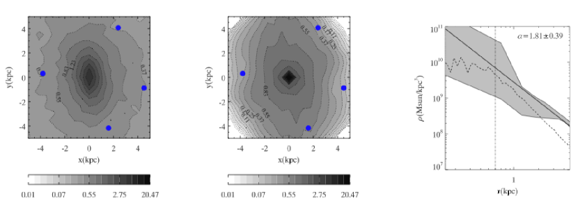
Figure 2: Recovered density distribution of the simulated galaxy, derived from the PixeLens mass map of one of the quads. Left: projected mass map for the simulated galaxy; the units for the contours are in units of the critical density. Middle: recovered projected mass map from PixeLens (see text for details). The solid circles show the distribution of (fake) images. Right: deprojected radial density distribution. The shaded gray region is the 68% confidence region. The oblique solid line is the best-fit power-law $r^{-\alpha}$. The dashed curve is the actual spherically-averaged $\rho(r)$. The plot is truncated at the projected radius of the outermost lens image. The vertical dot-dashed line to the left marks the resolution limit of the simulation—the apparent core to the left of this line is a result of the force softening and is not physical.

Figure 2, left and middle panels, show the 2D projected mass map of the simulated galaxy and the recovered distribution for one of the quads, respectively. Recall that all five mock lenses had the same mass map, but our modeling codes did not know that; the results from the other four galaxies were nearly identical to those presented here, and we omit these for brevity.

Notice how well the projected mass map is recovered. We obtain the correct elongation along the $y$-direction, while the contours of equal mass density are well-matched within the errors. Beyond the images (where we have no data) the mass distribution drops sharply and is not to be trusted; we do not use any data beyond the outer-most image in our deprojection.

Figure 3: $H_{0}^{-1}$ as recovered from the ten lens ensemble. The unbinned values give $15.2_{-1.7}^{+2.5}\,{\rm Gyr}$ ($H_{0}=64.3_{-9}^{+8}\,{\rm km\,s^{-1}\,Mpc^{-1}}$).

It is worth commenting a little on this plot. The mass map shown is the average of the full model ensemble; it represents the expectation value of the mass in each pixel. This does not mean, however, that it is not a genuine representation of the projected mass distribution. In this specific test here, PixeLens accurately recovers the input morphology and mass, within estimated uncertainties. In other similar examples in the literature, PixeLens has resolved substructure in lensing galaxies and clusters (Saha et al., 2007), and in one example, resolved an interacting pair of galaxies (see Paper I).

The deprojection of the recovered mass map is shown in the right panel of Figure 2. The simulated galaxy density profile (dashed line) is well recovered within the errors (grey band). Over-plotted is a power-law fit to the recovered density distribution, obtained using a standard Levenberg-Marquardt least-squares fitting technique (see e.g. Press et al. 1992). Note that, although this deprojection assumes spherical symmetry, our mass model up until this point did not (see also section 2.3).

3 Profiles of observed time-delay lenses

Having tested the pipeline of recovering both $H_{0}$ and $\rho(r)$ on mock lenses generated from a recent galaxy-formation simulation, we now derive radial profiles for real lenses.

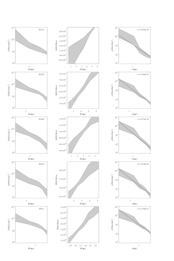
Figure 4: Inferred radial profiles for the lenses. The left column shows the projected density $\Sigma(R)$. The middle column shows the enclosed projected mass $M(R)$. The right column shows the deprojected density profiles $\rho(r)$ along with power-law fits $r^{-\alpha}$. The plots are truncated at the innermost and outermost image in each system. The gray bands are 68% uncertainties derived from the pixelated model ensembles and are probably a good representation of the uncertainties. The quoted uncertainties on $\alpha$ are formal 1$\sigma$ errors. These galaxies are all close to $\rho(r)\propto r^{-2}$. Continued in Figure 5.

The first part has already been done in Saha et al. (2006a) (Paper I), where a model-ensemble for ten time-delay lenses was generated, to estimate $H_{0}$. However, in this work we use a weaker prior and so it is worth plotting our determination of $H_{0}$ again. This is shown in Figure 3; the results are consistent with Paper I, and we recover $H_{0}^{-1}=15.2^{+2.5}_{-1.7}\,{\rm Gyr}$ ($H_{0}=64.3_{-9}^{+8}\,{\rm km\,s^{-1}\,Mpc^{-1}}$). Next, we derive $\rho(r)$, with uncertainties, from the model ensemble, as explained above. Finally we fit a power law $r^{-\alpha}$ to the non-parametric $\rho(r)$, as in section 2.4, above. Such a simple least-squares power law fit does not do justice to the full ensemble mass distribution which our non-parametric method derives for each galaxy. We use it just as a convenient way of representing our results on a single plot (Figure 6), and as a simple way to compare our results with theoretical expectations. Our detailed results are shown in Figures 4 and 5.

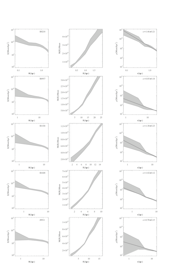
Figure 5: Continuation of Figure 4. The lenses shown here are all significantly shallower than $r^{-2}$.

Figure 6 then summarizes the log density slopes, $\alpha$, for all ten lenses. Five are close to $r^{-2}$ or slightly steeper, and five are shallower, clustering around $\sim r^{-1}$. Formal errors on $\alpha$ are shown by the error bars. These probably somewhat underestimate the actual uncertainties.

Figure 6: The mean steepness, $\alpha$ (where $\rho\propto r^{-\alpha}$), for the ten lensing galaxies. Formal errors are marked.

The five systems close to $r^{-2}$ are all relatively isolated galaxies (though nearby galaxies contributing some external shear are often present). From estimates of the stellar mass through population synthesis models (Ferreras et al., 2005), all five have both stars and dark matter contributing to lensing. In other words, these are all galaxies where we would expect an isothermal mass distribution.

The five shallower lenses are different. In B0957+561 and J0911+055 the main lensing galaxy is in a cluster, while B0218+357 and B1104+180 have little starlight, suggesting a dark-matter dominated lens; in all of these cases we would expect a shallower profile than $r^{-2}$. Finally, in B1608+656 the lens consists of two interacting galaxies; here the density peak of the host galaxy will be averaged with the lower density material from the infalling system, hence here again we would expect a shallower profile than $r^{-2}$.

It is worth adding an extra comment for B0218+357, which appears distinct from the other lenses. Our five steep lenses have the outer-most image at a projected radius of $<10$ kpc. By contrast, all of the shallow lenses have the outer-most image at $>10$ kpc, with the exception of B0218+357. B0218+357 has its outermost image at a projected radius of little over $\sim 2$ kpc, while its profile is of intermediate steepness, with $\alpha\sim 1.5$. It may be that these peculiarities are the result of a poor determination of the optical centre for this lens, due its small size on the sky (2003MNRAS.338..599B). Such errors are not currently taken into account in our models. We hope to investigate this lens in more detail in future work.

We conclude that while the inferred steepness has a large uncertainty, the identification of nearly $r^{-2}$ versus shallower profiles is a strong result.

4 Comparison with previous work

Some recent work has concluded that if measured time delays are to be consistent with $H_{0}^{-1}\simeq 14\,{\rm Gyr}$ ($H_{0}\simeq 70\,{\rm km\,s^{-1}\,Mpc^{-1}}$) then the galaxy mass profiles involved must be significantly steeper than $r^{-2}$. In particular, Kochanek & Schechter (2004) find that isothermal lenses give $H_{0}^{-1}=20\pm 1\,{\rm Gyr}$ ($H_{0}=48\pm 3\,{\rm km\,s^{-1}\,Mpc^{-1}}$) from the measured time delays. Dobke & King (2006) report that $H_{0}=71\,{\rm km\,s^{-1}\,Mpc^{-1}}$ is consistent with an $r^{-2}$ profile within $3\sigma$. However, when they separate the lens sample into doubles and quads, the $3\sigma$ uncertainties do not overlap, so it is not clear how to interpret their result. Koopmans et al. (2006) attempt to break the steepness degeneracy using a single velocity dispersion for each galaxy. They conclude that all of their sample (time delays are not available for those lenses) is consistent within observational errors with isothermal profiles. However, when the same method is applied to the time-delay lens B1115+080 (Treu & Koopmans, 2002) a profile significantly steeper than isothermal is inferred. See Dobke et al. (2007) for a recent discussion of the difficulties and proposed solutions.

Figure 7: Distribution of reduced time delays, $\Xi$ [see equation A9], for the simulated galaxy lens (solid histogram). To produce this plot we traced rays from a uniform distribution of sources in the source-plane and calculated the distribution of arrival times for their images in the image plane. Over-plotted are the similar results for an isothermal lens (solid vertical line) and a first-order perturbed isothermal lens (Equation 8, with $\epsilon=0.15\theta_{\mathrm{E}}$; dotted line). The latter two are calculated analytically in section 5. Since an isothermal lens has $\Xi=1$, this plot measures the deviation of time delays from isothermal.

Somewhat in contrast is the work of Ferreras et al. (2005), who compared stellar-mass profiles derived from population synthesis models with total-mass profiles reconstructed using PixeLens for 18 early-type lensing galaxies, of which six had time-delay measurements (all also used in the present work). Although that paper does not discuss the steepness of the profiles as such, it finds no inconsistencies when the measured time-delays were imposed as constraints along with $H_{0}^{-1}=14\,{\rm Gyr}$. Plausible dark-matter fractions are inferred for all the lenses, and the tilt of the fundamental plane is reproduced.

The above studies all use different (though sometimes overlapping) samples of lenses. This is not a problem for pixelated models, since the method explicitly allows for heterogeneous samples. However, in studies that assume a simple form for lensing galaxies, sample selection becomes an issue and may be partly responsible for differences between results for $H_{0}$ and density profiles presented in the literature so far. However, as we shall now demonstrate, the details of the mass model have a far more important effect.

Figure 7 shows the distribution of reduced time delays $\Xi$ [see Equation A9] for the simulated lens with a uniform distribution of sources (solid histogram). Although the simulated lens is well-fit by an isothermal density distribution (Figure 2), its distribution of reduced time delays is not.

5 Time delays in a perturbed isothermal lens

The unexpectedly broad histogram in Figure 7 is readily understood from a perturbative calculation, as we now show.

Consider an isothermal lens with Einstein radius $\theta_{\mathrm{E}}$, with a source at $(p,0)$. As is well known, the arrival time at sky position $(x,y)$ is

$$\tau(x,y)={\textstyle\frac{1}{2}}(x-p)^{2}+{\textstyle\frac{1}{2}}y^{2}-\theta_{\mathrm{E}}\sqrt{x^{2}+y^{2}}.$$ (3)

Equating the gradient of $\tau$ to zero gives the image positions (provided $|p|<\theta_{\mathrm{E}}$)

$$x_{+}=p+\theta_{\mathrm{E}},\quad x_{-}=p-\theta_{\mathrm{E}},\quad y_{\pm}=0.$$ (4)

Here $(x_{+},0)$ is a minimum, $(x_{-},0)$ is a saddle point, and there is no third image because the potential is singular. For $p=0$ the two images merge into an Einstein ring.

Plugging the image positions back into Equation (3), we obtain the time delay

$$\tau_{-}-\tau_{+}=2p\,\theta_{\mathrm{E}}.$$ (5)

Note that $\tau_{+}<\tau_{-}$. It is easily verified that the reduced time delay (A9) is unity.

Now imagine that we add a perturbing potential $\delta\Phi$ to Equation (3). As is usual in perturbation theory, we Taylor expand about the unperturbed solution.

$$\delta\Phi_{\pm}=\epsilon_{\pm}x+\epsilon^{\prime}_{\pm}y+O(\epsilon^{2})$$ (6)

where $\epsilon_{\pm}$ and $\epsilon^{\prime}_{\pm}$ are Taylor-expansion coefficients around the two images $(x_{\pm},0)$. Equating the gradient of the perturbed arrival time $\tau-\delta\Phi$ to zero, we have to first order:

$$x_{\pm}=p\pm\theta_{\mathrm{E}}+\epsilon_{\pm},\quad y_{\pm}=\epsilon^{\prime}_{\pm}(1\pm\theta_{\mathrm{E}}/p).$$ (7)

We now write $\epsilon$ for the mean of $\epsilon_{\pm}$ and neglect their difference. The numerator in the reduced time delay (A9) remains $2p\,\theta_{\mathrm{E}}$ to leading order, whereas the denominator is now $2(p+\epsilon)\,\theta_{\mathrm{E}}$. Hence we have

$$\Xi=\left(1+\frac{\epsilon}{p}\right)^{-1}.$$ (8)

Now comes the key point. Since $p$ can be small, $\epsilon/p$ need not be small. Hence small perturbations of an isothermal lens can produce zeroth-order changes in the reduced time delay.

In Figure 7 we have over-plotted the distribution of $\Xi$ for $\epsilon=0.15\,\theta_{\mathrm{E}}$ (dotted line). For this computation, we had $\sqrt{p}$ uniformly distributed, corresponding to a uniform distribution of sources in a disk. There is a gap in the perturbed distribution around $\Xi=1$, which arises because $|p|<\theta_{\mathrm{E}}$. Otherwise, however, our simple first-order perturbative calculation qualitatively reproduces the distribution for the simulated galaxy, including the asymmetry.

The sensitivity of the time delays to perturbations of the lens has been noted in the literature before. Witt et al. (2000) studied perturbations of the isothermal lens, and found that a shear perturbation could produce a large change in the time delays. Similarly, Oguri (2006) considered more general perturbations to the isothermal sphere and found that perturbations to the isothermal potential can give large changes in the time delays – indeed our result is implicit in their Figure 1. However, these works did not stress the importance of comparing perturbations to the time delays against perturbations to the image positions. Only Blandford & Narayan (1986) appear to have commented directly on this: “It has been our experience that fairly small changes in the lensing potential may introduce much larger difference in the delays than in the image properties.”

6 Conclusions

Our main result on density slopes (shown in Figures 4 and 5, and summarized in Figure 6) is that five of the galaxies studied are close to $\rho\propto r^{-2}$, whereas the other five are shallower and clustered around $\rho\propto r^{-1}$. The former are all relatively isolated galaxies where stars and dark matter probably both contributing significantly to lensing. The shallow systems are different: B0957+561 and J0911+055 lie in clusters; in B1104–181 the lens images are far out in the halo suggesting that this lens is probably dark-matter dominated; B0218+357 has little starlight, suggesting also a dark-matter dominated lens, though the centroid is difficult to determine for this system; and finally B1608+656 is a pair of interacting galaxies. Thus the latter five are just those systems which we might have guessed would be shallower. Our technique is tested on a mock survey of five lenses generated from a galaxy-formation simulation, from which $H_{0}$ and the mass profile are both recovered within the claimed uncertainties (Figures 1 and 2).

A significant finding is that, when calculating time delays:

$$\hbox{a nearly-isothermal {\it mass distribution}}\not\simeq\hbox{a perfect isothermal lens}.$$ (9)

We demonstrate this through a simple perturbation calculation showing how a small deviation from an isothermal potential can be amplified in the time delays. We also verify this effect in a simulated galaxy, where time delays from 0.5 to 2 (and, in rare cases, an arbitrarily large number) times the value expected for a isothermal lens can occur (Fig. 7), depending on the source position.

Although fleetingly anticipated by Blandford & Narayan (1986) and suggested by some more recent modeling work (Bernstein & Fischer, 1999; Zhao & Qin, 2003; Saha & Williams, 2006), the assertion (9) is contrary to the majority of lens models so far. Such models assume that lensing time delays are completely determined by the image positions and radial power-law index. Once we drop that invalid approximation, the apparent contradictions between time delays and mass profiles much discussed in several recent papers (see Section 4) are resolved.

7 Acknowledgements

We thank Jonathan Coles for providing the latest version of PixeLens.

Appendix A Lensing theory: scales and degeneracies

This paper makes use of a number of rather specialized results from lensing theory. These are well-known known to experts, but since the original derivations are spread over diverse papers and a long time span, we review them here.

A.1 The arrival-time surface

We start with the expression for the change in travel time for a virtual photon originally from a source at sky position $\hbox{\boldmath{$\theta$}}_{\hbox{\tiny{S}}}$ but deflected at the lens so that the observer sees it coming from sky-position $\hbox{\boldmath{$\theta$}}_{\hbox{\tiny{I}}}$:

$$c\,t(\hbox{\boldmath{$\theta$}}_{\hbox{\tiny{I}}};\hbox{\boldmath{$\theta$}}_{\hbox{\tiny{S}}})=(1+z_{\hbox{\tiny{L}}})\frac{d_{\hbox{\tiny{OL}}}d_{\hbox{\tiny{OS}}}}{2d_{\hbox{\tiny{LS}}}}(\hbox{\boldmath{$\theta$}}_{\hbox{\tiny{I}}}-\hbox{\boldmath{$\theta$}}_{\hbox{\tiny{S}}})^{2}-(1+z_{\hbox{\tiny{L}}})\frac{4G}{c^{2}}\int\Sigma(\hbox{\boldmath{$\theta$}}^{\prime})\ln|\hbox{\boldmath{$\theta$}}_{\hbox{\tiny{I}}}-\hbox{\boldmath{$\theta$}}^{\prime}|\,d^{2}\hbox{\boldmath{$\theta$}}^{\prime}.$$ (A1)

This is just Equation (2.6) from Blandford & Narayan (1986) with all the dimensions put back in; as in that paper, $\Sigma$ is the sky-projected density, $z_{\hbox{\tiny{L}}}$ is the lens redshift, $d_{\hbox{\tiny{OL}}}$ is the angular-diameter distance from observer to lens, and so on. The first term on the right is the geometrical path difference between a deflected and undeflected photon trajectory, and the last term is the general-relativistic delay. The above equation assumes that the lens is a) infinitesimally thin (compared to $d_{\hbox{\tiny{OL}}}$ and $d_{\hbox{\tiny{LS}}}$), and b) lies in a representative patch of the Universe (Blandford & Narayan, 1986). Both of these are conservative assumptions.

The light-travel time (A1) can be expressed in a useful dimensionless form by some substitutions. First, we have the scaled time variable

$$\tau=\left[(1+z_{\hbox{\tiny{L}}})\frac{d_{\hbox{\tiny{OL}}}d_{\hbox{\tiny{OS}}}}{d_{\hbox{\tiny{LS}}}}\right]^{-1}c\,t.$$ (A2)

Each of $d_{\hbox{\tiny{OL}}},d_{\hbox{\tiny{OS}}},d_{\hbox{\tiny{LS}}}$ is $(c/H_{0})$ times a redshift- and cosmology-dependent factor of order unity. In other words

$$\tau\sim H_{0}^{-1}t$$ (A3)

or the time delay in units of the Hubble time. Next, we introduce the dimensionless distance factor

$$c_{\hbox{\tiny{LS}}}=\frac{d_{\hbox{\tiny{LS}}}}{d_{\hbox{\tiny{OS}}}}.$$ (A4)

Then we consider

$$\kappa=\frac{4\pi G}{c^{2}}d_{\hbox{\tiny{OL}}}\Sigma$$ (A5)

which can be interpreted as $\Sigma$ in units of the critical density for sources at infinity. (In many papers, the $c_{\hbox{\tiny{LS}}}$ factor is absorbed inside the definition of $\kappa$; that refers $\kappa$ to a particular $z_{\hbox{\tiny{S}}}$.) Finally, we write an operator that solves Poisson’s equation in two dimensions

$$\nabla^{-2}f\equiv\frac{1}{2\pi}\int f(\hbox{\boldmath{$\theta$}}^{\prime})\ln|\hbox{\boldmath{$\theta$}}_{\hbox{\tiny{I}}}-\hbox{\boldmath{$\theta$}}^{\prime}|\,d^{2}\hbox{\boldmath{$\theta$}}^{\prime}.$$ (A6)

With all these substitutions we obtain

$$\tau(\hbox{\boldmath{$\theta$}}_{\hbox{\tiny{I}}};\hbox{\boldmath{$\theta$}}_{\hbox{\tiny{S}}})={\textstyle\frac{1}{2}}(\hbox{\boldmath{$\theta$}}_{\hbox{\tiny{I}}}-\hbox{\boldmath{$\theta$}}_{\hbox{\tiny{S}}})^{2}-2c_{\hbox{\tiny{LS}}}\nabla^{-2}\kappa(\hbox{\boldmath{$\theta$}}_{\hbox{\tiny{I}}}).$$ (A7)

For given $\hbox{\boldmath{$\theta$}}_{\hbox{\tiny{S}}}$, the abstract surface $\tau(\hbox{\boldmath{$\theta$}}_{\hbox{\tiny{I}}})$ is called the arrival-time surface. It is abstract because real photons do not arrive from all $\hbox{\boldmath{$\theta$}}_{\hbox{\tiny{I}}}$ — they arrive only from $\hbox{\boldmath{$\theta$}}_{\hbox{\tiny{I}}}$ that make $\tau(\hbox{\boldmath{$\theta$}}_{\hbox{\tiny{I}}})$ extremal (Fermat’s principle). In other words, images appear where the arrival-time surface has a maximum, minimum, or saddle-point.

A.2 Dimensionless time delays

Equation (A7) is completely dimensionless if we measure angles in radians, which emphasizes that a lens model $\kappa(\hbox{\boldmath{$\theta$}}_{\hbox{\tiny{I}}})$ on its own is dimensionless. Scales in lensing enter through equations (A2), (A4) and (A5), which are all model-independent. (See Nityananda, 1990, for an interesting discussion of this point.)

The last statement may seem paradoxical. If lens models are dimensionless, how can a lens model help infer $H_{0}$? The resolution is that lens models relate two time scales —$H_{0}^{-1}$ and observable time delays— even though they have no time scales of their own. Because of this, we can speak of a dimensionless time delay even for an observed lens with a measured time delay, and this is very useful for comparing a heterogeneous set of lenses. Two ways of turning a measured delay $\Delta t$ into a dimensionless number are suggested in Saha (2004).

One possibility is to compute

$$\varphi=\frac{\Delta t}{{\textstyle\frac{1}{16}}(\theta_{1}+\theta_{2})^{2}D}$$ (A8)

where where $\theta_{1},\theta_{2}$ are the lens-centric distances (in radians) of the first and last images to arrive, $\Delta t$ is the observed time delay between them, and $D$ is the factor $(1+z_{\hbox{\tiny{L}}})(d_{\hbox{\tiny{OL}}}d_{\hbox{\tiny{OS}}}/d_{\hbox{\tiny{LS}}})$ from equation (A2) — which recall is $\propto H_{0}^{-1}$. The factor $\frac{1}{16}(\theta_{1}+\theta_{2})$, with angles in radians, is approximately (exactly for an isothermal lens) the fraction of the sky covered by the Einstein ring. It turns out that $\varphi$ lies in the range $\simeq[0,2]$ for doubles and $\simeq[2,8]$ for quads. This property was exploited by Saha et al. (2006a) to compare observed and $N$-body time delays.

Another possibility is the reduced time delay

$$\Xi=\frac{\Delta t}{{\textstyle\frac{1}{2}}(\theta_{1}^{2}-\theta_{2}^{2})D}$$ (A9)

which has a wider range than $\varphi$ but has the attractive property that for an isothermal lens $\Xi=1$. Oguri (2006) uses $\Xi$ as a basis to compare the distributions of observed and model time delays; we also use this quantity in section 5.

A.3 Steepness and other degeneracies

Let us rewrite the arrival time slightly as

$$\tau=2\,\nabla^{-2}(1-c_{\hbox{\tiny{LS}}}\kappa)-\hbox{\boldmath{$\theta$}}_{\hbox{\tiny{I}}}\cdot\hbox{\boldmath{$\theta$}}_{\hbox{\tiny{S}}}$$ (A10)

where we have used the fact that in two dimensions $\nabla^{2}\theta^{2}=4$, and also discarded a $\hbox{\boldmath{$\theta$}}_{\hbox{\tiny{S}}}^{2}$ term since it has no optical effect. Now consider the rescaling

$$\tau^{\prime}=\lambda\tau,\quad(1-c_{\hbox{\tiny{LS}}}\kappa^{\prime})=\lambda(1-c_{\hbox{\tiny{LS}}}\kappa),\quad\hbox{\boldmath{$\theta$}}_{\hbox{\tiny{S}}}^{\prime}=\lambda\hbox{\boldmath{$\theta$}}_{\hbox{\tiny{S}}}.$$ (A11)

applied to Equation (A10), where $\lambda$ is constant in the region of images. There is no effect on the image positions or relative magnifications — basically we are redefining the contour spacing in a contour map of the arrival-time surface (such as Blandford & Narayan’s Figure 2) without altering the figure. However, time delays change because $\tau$ is rescaled, while the total magnification changes because $\hbox{\boldmath{$\theta$}}_{\hbox{\tiny{S}}}$ is rescaled. Meanwhile, rescaling $(1-c_{\hbox{\tiny{LS}}}\kappa)$ means that the mass profile gets steeper (if $\lambda>1$) or shallower (if $\lambda<1$).

Equation (A11) is the well-known steepness degeneracy. The simple geometric derivation given here is from Saha (2000), but it was first derived by a different method by Falco et al. (1985).

The steepness degeneracy is broken if there is a range of $z_{\hbox{\tiny{S}}}$ (Abdelsalam et al., 1998b; Saha et al., 2006c). That is because a range of $z_{\hbox{\tiny{S}}}$ gives a range of $c_{\hbox{\tiny{LS}}}$, and Equation (A11) can only be applied if $c_{\hbox{\tiny{LS}}}$ is constant. Another way to break the degeneracy is to have number counts of weakly lensed objects (Dye et al., 2002) because then the total magnification is constrained and $\hbox{\boldmath{$\theta$}}_{\hbox{\tiny{S}}}$ cannot be freely rescaled. However for galaxy lenses, neither of these routes is in practice available. Multiple sources at the same $z_{\hbox{\tiny{S}}}$ do not help here, since the rescaling (A11) can be applied to multiple sources, so even an Einstein ring does not break the degeneracy (Saha & Williams, 2001).

That the steepness degeneracy is a serious problem for galaxy lenses is now widely appreciated, and researchers agree that steeper mass profiles lead to larger values of $(H_{0}\,\Delta t)$. But as our Figure 7 shows, significant degeneracies can persist even at fixed slope. These degeneracies appear to consist of rescalings of the type (A11) but with varying $\lambda$. The details remain to be investigated.

References

- Abdelsalam et al. (1998a) Abdelsalam, H. M., Saha, P., & Williams, L. L. R. 1998a, MNRAS, 294, 734
- Abdelsalam et al. (1998b) —. 1998b, AJ, 116, 1541
- Bernstein & Fischer (1999) Bernstein, G. & Fischer, P. 1999, AJ, 118, 14
- Blandford & Narayan (1986) Blandford, R. & Narayan, R. 1986, ApJ, 310, 568
- Bradač et al. (2005) Bradač, M., Schneider, P., Lombardi, M., & Erben, T. 2005, A&A, 437, 39
- Diego et al. (2005) Diego, J. M., Sandvik, H. B., Protopapas, P., Tegmark, M., Benítez, N., & Broadhurst, T. 2005, MNRAS, 362, 1247
- Diemand et al. (2004) Diemand, J., Moore, B., & Stadel, J. 2004, MNRAS, 353, 624
- Dobke & King (2006) Dobke, B. M. & King, L. J. 2006, A&A, 460, 647
- Dobke et al. (2007) Dobke, B. M., King, L. J., & Fellhauer, M. 2007, ArXiv Astrophysics e-prints
- Dye et al. (2002) Dye, S., Taylor, A. N., Greve, T. R., Rögnvaldsson, Ö. E., van Kampen, E., Jakobsson, P., Sigmundsson, V. S., Gudmundsson, E. H., & Hjorth, J. 2002, A&A, 386, 12
- Falco et al. (1985) Falco, E. E., Gorenstein, M. V., & Shapiro, I. I. 1985, ApJ, 289, L1
- Ferreras et al. (2005) Ferreras, I., Saha, P., & Williams, L. L. R. 2005, ApJ, 623, L5
- Graham et al. (2006a) Graham, A. W., Merritt, D., Moore, B., Diemand, J., & Terzić, B. 2006a, AJ, 132, 2701
- Graham et al. (2006b) —. 2006b, AJ, 132, 2711
- Hayashi et al. (2004) Hayashi, E., Navarro, J. F., Power, C., Jenkins, A., Frenk, C. S., White, S. D. M., Springel, V., Stadel, J., & Quinn, T. R. 2004, MNRAS, 355, 794
- Humphrey et al. (2006) Humphrey, P. J., Buote, D. A., Gastaldello, F., Zappacosta, L., Bullock, J. S., Brighenti, F., & Mathews, W. G. 2006, ApJ, 646, 899
- Kazantzidis et al. (2004) Kazantzidis, S., Kravtsov, A. V., Zentner, A. R., Allgood, B., Nagai, D., & Moore, B. 2004, ApJ, 611, L73
- Keeton & Winn (2003) Keeton, C. R. & Winn, J. N. 2003, ApJ, 590, 39
- Kochanek & Schechter (2004) Kochanek, C. S. & Schechter, P. L. 2004, in Measuring and Modeling the Universe, ed. W. L. Freedman, 117–+
- Koopmans et al. (2006) Koopmans, L. V. E., Treu, T., Bolton, A. S., & Moustakas, L. A. 2006, ApJ, 649, 599
- Kronawitter et al. (2000) Kronawitter, A., Saglia, R. P., Gerhard, O., & Bender, R. 2000, A&AS, 144, 53
- Lynden-Bell (1967) Lynden-Bell, D. 1967, MNRAS, 136, 101
- Macciò (2005) Macciò, A. V. 2005, MNRAS, 361, 1250
- Macciò et al. (2006) Macciò, A. V., Moore, B., Stadel, J., & Diemand, J. 2006, MNRAS, 366, 1529
- Mayer (2004) Mayer, L. 2004, in Proceedings of ”Baryons in Dark Matter Halos”. Novigrad, Croatia, 5-9 Oct 2004. Editors: R. Dettmar, U. Klein, P. Salucci. Published by SISSA, Proceedings of Science, http://pos.sissa.it, p.37, 37–+
- Merritt et al. (2006) Merritt, D., Graham, A. W., Moore, B., Diemand, J., & Terzić, B. 2006, AJ, 132, 2685
- Moore et al. (1998) Moore, B., Governato, F., Quinn, T., Stadel, J., & Lake, G. 1998, ApJ, 499, L5+
- Navarro et al. (1996) Navarro, J. F., Frenk, C. S., & White, S. D. M. 1996, ApJ, 462, 563
- Nityananda (1990) Nityananda, R. 1990, Current Science, 50, 1044
- Oguri (2006) Oguri, M. 2006, ArXiv Astrophysics e-prints
- Press et al. (1992) Press, W. H., Teukolsky, S. A., Vetterling, W. T., & Flannery, B. P. 1992, Numerical recipes in C. The art of scientific computing (Cambridge: University Press, —c1992, 2nd ed.)
- Raychaudhury et al. (2003) Raychaudhury, S., Saha, P., & Williams, L. L. R. 2003, AJ, 126, 29
- Saha (2000) Saha, P. 2000, AJ, 120, 1654
- Saha (2004) —. 2004, A&A, 414, 425
- Saha et al. (2006a) Saha, P., Coles, J., Macciò, A. V., & Williams, L. L. R. 2006a, ApJ, 650, L17
- Saha et al. (2006b) Saha, P., Courbin, F., Sluse, D., Dye, S., & Meylan, G. 2006b, A&A, 450, 461
- Saha et al. (2006c) Saha, P., Read, J. I., & Williams, L. L. R. 2006c, ApJ, 652, L5
- Saha & Williams (1997) Saha, P. & Williams, L. L. R. 1997, MNRAS, 292, 148
- Saha & Williams (2001) —. 2001, AJ, 122, 585
- Saha & Williams (2004) —. 2004, AJ, 127, 2604
- Saha & Williams (2006) —. 2006, ApJ, 653, 936
- Saha et al. (2007) Saha, P., Williams, L. L. R., & Ferreras, I. 2007, Meso-structure in three strong-lensing systems
- Shu (1991) Shu, F. 1991, Physics of Astrophysics, Vol. II: Gas Dynamics (Published by University Science Books, 648 Broadway, Suite 902, New York, NY 10012, 1991.)
- Treu & Koopmans (2002) Treu, T. & Koopmans, L. V. E. 2002, MNRAS, 337, L6
- van der Marel (1991) van der Marel, R. P. 1991, MNRAS, 253, 710
- White & Rees (1978) White, S. D. M. & Rees, M. J. 1978, MNRAS, 183, 341
- Williams & Saha (2000) Williams, L. L. R. & Saha, P. 2000, AJ, 119, 439
- Witt et al. (2000) Witt, H. J., Mao, S., & Keeton, C. R. 2000, ApJ, 544, 98
- Young (1980) Young, P. 1980, ApJ, 242, 1232
- Zhao & Qin (2003) Zhao, H. & Qin, B. 2003, ApJ, 582, 2