On Bounds and Algorithms for Frequency Synchronization for Collaborative Communication Systems
Abstract
Cooperative diversity systems are wireless communication systems designed to exploit cooperation among users to mitigate the effects of multipath fading. In fairly general conditions, it has been shown that these systems can achieve the diversity order of an equivalent MISO channel and, if the node geometry permits, virtually the same outage probability can be achieved as that of the equivalent MISO channel for a wide range of applicable SNR. However, much of the prior analysis has been performed under the assumption of perfect timing and frequency offset synchronization. In this paper, we derive the estimation bounds and associated maximum likelihood estimators for frequency offset estimation in a cooperative communication system. We show the benefit of adaptively tuning the frequency of the relay node in order to reduce estimation error at the destination. We also derive an efficient estimation algorithm, based on the correlation sequence of the data, which has mean squared error close to the Cramér-Rao Bound.
I Introduction
Collaborative communication systems employ cooperation among nodes in a wireless network to increase data throughput and robustness to signal fading. Much of the research done in this area has concentrated on information theoretic results, protocols, and coding while assuming perfect synchronization [1, 2, 3, 4, 5, 6]. In this paper, we explore frequency synchronization of a collaborative system and provide estimation bounds and practical algorithms having performance close to the bounds.
In a collaborative system, nodes that would have remained silent during some period of time adapt to their surroundings and collaborate with the source and destination nodes. These systems, sometimes termed cooperative diversity systems, use distributed protocols to greatly improve performance over traditional point-to-point communication systems. One improvement to system performance comes in the form of added robustness to signal fading [1, 2]. An effective way to achieve robustness is to increase the spatial diversity by using multiple antennas as in a MIMO system [7, 8]. However, when considering a network of low-cost wireless devices, the size and cost of multiple antennas is prohibitive for these devices [9]. A way for low cost nodes to realize much of the benefit of a MIMO system is through collaborative (cooperative) diversity. In fact, in [1] it is shown that a collaborative system can have the same diversity order as an equivalent MISO system. Employing a collaborative protocol in a wireless network can also increase the overall throughput of the network. The use of relaying is a special case of network coding and as shown in [10], the capacity of a relay (or coded) network is greater than in a traditional point-to-point network.
To design a practical collaborative communication system, one of two methods may be used. The signal modulation and coding may be designed to be naturally robust to synchronization errors [11], or alternatively, the frequency and timing offsets are estimated and subsequently compensated [12]. We explore the second option in this paper. Algorithms and bounds for standard synchronization are found in [13, 14, 15]. The related case of a MIMO channel with multiple frequency offsets is treated in [16, 17]. In this paper, we provide more details and extend the results of [18]. We derive the transmission frequency the relay must use to optimally reduce the variance of the frequency estimator at the destination by minimizing the Cramér-Rao Bound (CRB) of the frequency estimators at each receive node. By using the CRB, our frequency selection algorithm is independent of algorithm choice. We also provide an efficient frequency estimation algorithm for the collaborative system.
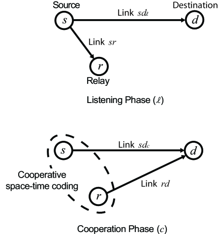
In [12], Shin et. al. describes a specific protocol, which we use in this paper, for collaborative communication with synchronization among three nodes: a source, a relay, and a destination. The protocol is based on a two-phase transmission within each frame [1, 4], a listening phase and a cooperation phase. Within each phase there is a preamble containing synchronization signals. In the listening phase, the relay receives and decodes the source’s message. During the cooperation phase, the relay re-encodes and transmits the message cooperatively with the source. This process is illustrated in Figure 1.
The synchronization algorithms in [12] are ad-hoc and meant only to serve as a proof-of-concept that synchronization is possible with collaborative systems. In this paper, we derive the CRB for optimal frequency offset estimation for the class of systems discussed above. We show there exists an optimal (with respect to minimizing the CRB) frequency of transmission for the relay node based on: 1) the accuracy of estimation during the listening phase and 2) the SNR of all node pairs. We derive the maximum-likelihood (ML) frequency estimators for each receive node. These estimators are asymptotically efficient, meaning they achieve the CRB at high signal-to-noise ratio (SNR). However, the ML solution is computationally expensive and we therefore derive a practical correlation based estimation algorithm with performance close to the CRB. For the purposes of this paper, we assume a frequency selective fading model and that timing synchronization has been performed. Future papers will extend this work to include timing estimation and synchronization. We also assume all training sequences are constant modulus signals.
This paper is organized as follows, Section II outlines the mathematical model describing the signals involved in the frequency estimation portion of each phase. The CRB and ML estimators are derived in Sections III and IV for the listening and cooperation phases respectively. Section V provides some simulation results to illustrate the behavior and performance of frequency estimation in the three node relay system while Section VI shows the mean squared error (MSE) performance of each algorithm as compared with the CRB.
The following notation is used throughout: italic letters () represents scalar quantities, bold lowercase letters () represent vectors, bold uppercase letters () represent matrices, denotes transpose, denotes complex conjugation, denotes complex conjugate transpose, denotes the 2-norm of a vector, denotes the real part of a complex number, denotes the expectation operator with respect to the random variable , represents the Gaussian distribution with mean and variance and represents the circularly symmetric complex Gaussian distribution, i.e., where the real and imaginary parts are independent and identically distributed Gaussian random variables with variance .
II System Model
The system model is defined in this section. During each phase, a preamble consisting of a certain number of samples ( for listening and for cooperation) used for frequency synchronization. We assume the transmission channel is frequency selective with channel impulse response samples long. Due to differences in local oscillator characteristics, the operating frequency of each node is slightly different. Let denote the operating frequency of the source node and similar definitions for and . The notation is used to denote the source to destination link and likewise for and . As link is used in each phase, let denote the link during the listening phase and be for the cooperation phase.
Each transmitted signal is received and converted to baseband for subsequent processing. During the listening phase, the baseband signal of link is expressed as [15]
| (1) |
where is the sample index, is the frequency offset between the two nodes of link normalized by the sample rate, is the noise generated in the electronics of receiver (destination or relay node respectively), and is the combination of the known training signals () and the effects of the frequency selective channel, given by
In this equation, are the samples of the channel response for link and is the duration of the channel response. We assume, for each link , the length of the channel is the same. Writing (1) in matrix form gives
| (2) |
where is a diagonal matrix and is a Toeplitz matrix where for and .
In the cooperation phase, the signal is defined as follows,
| (3) |
where we assume the frequency is constant over both phases. For each receiver, , the noise is assumed to be a zero-mean circularly symmetric complex Gaussian random vector
In the general case, the frequency offsets between nodes can take on any values within the Doppler spread of the system plus the frequency differences of the local oscillators. We assume the maximum frequency offset is bounded and use this information to calculated the CRB and ML frequency estimators. In the remainder of the paper, we assume the nodes are stationary and thus the signals have no Doppler spread. A statistical model for the frequency offset is used as prior information to aid in frequency estimation. Let the operating frequency of each node be modeled as
where is the mean operating frequency and is a random variable with mean zero and variance . We assume the random variables are independent. For this paper, we also assume for all nodes , which is an appropriate model when considering a group of identical nodes cooperating together. The frequency offsets to be estimated are the difference between two of these independent random variables and thus the frequencies, for , have mean zero, variance , and are correlated.
III Listening Phase
In the listening phase, the destination and the relay receive the same signal through two different channels. We drop the subscript when considering only the single node-to-node link. To derive a good estimator for the frequency, it is useful to know the distribution of . However, this is not known, so it is reasonable to design an estimator based on the “worst case” distribution constrained to the known statistics, i.e., a mini-max estimator. As frequency estimation is inherently non-linear, an asymptotic analysis is performed in the high SNR regime (i.e., SNR). Under this assumption, the variance of a ML or maximum a posteriori (MAP) estimator is equal to the CRB. In the remainder of this section, we show that a Gaussian distribution with mean zero and variance for maximizes the CRB of the frequency estimate over all distributions with the same mean and variance. We then derive the MAP estimator of .
III-A Cramér-Rao Bound
The unknown parameters in the single node-pair model (1) are (which is modeled as a random variable with mean zero and variance ) and .111The parameter is considered known as it is a property of the receiver hardware. Also, the noise variance is uncoupled with the other parameters and is estimated separately with no penalty. The CRB is defined to be the diagonal entries of the inverse Fisher Information Matrix (FIM). When one or more parameters are random variables, the FIM is expressed in the following form [19]
| (4) |
where the expectation is taken over the random variable ,
is the standard (non-random parameter) FIM, with expectation over the noise distribution, and is the log-likelihood of the data vector when the values of and are held constant. The matrix is defined as follows:
where and is the distribution function of the random variable . For the parameter vector , the FIM has the following form [20]
| (5) |
where is a scalar in this case. Let be a diagonal matrix such that
| (6) |
The submatrices of (5) are computed as
None of these components depend on the random variable and therefore the expectation in (4) goes away. The matrix is only non-zero in the first element and is
| (7) |
where is the Fisher information of the random variable and is the log-likelihood of . The CRB for an estimator of is then , which can be calculated using the Shur complement222The block of a block matrix inverse is . [21] to be
where is the projection matrix onto the space orthogonal to the range of . As the Fisher information is a positive number, it is clear that, to find the worst case (maximum) CRB, must be minimized. We use the following Lemma to show how this variable is minimized.
Lemma 1
Let represent the family of distributions with mean zero and variance . Let be a random variable distributed as . The minimum of the Fisher information of , as defined in (7), over the family of distributions with variance is achieved when
Proof: Consider the following experiment: without any data, design an estimator for the random variable . The log-likelihood in this case is . If , then this estimator is unbiased and its variance is . By the Cramér-Rao Theorem,
Therefore, with equality being achieved when . ∎
By Lemma 1, the maximum CRB (over all distributions of with variance ) is
| (8) |
III-B MAP Estimator of frequency
As a result of the preceding analysis, we use a Gaussian prior distribution on to calculate the MAP estimator. This choice of prior represents the least informative prior of all distributions with variance and mean zero. For a particular channel gain , the log-likelihood of the data is
| (9) |
The apparent additional factor of two associated with is due to the fact that has a real Gaussian distribution as opposed to complex (as in the first term above). For any given frequency, the maximum of this expression over is achieved when
| (10) |
To find the MAP estimator of , we substitute (10) into (9) and minimize the negative,
| (11) |
We note that as goes to infinity (no prior information), the estimator (11) is the standard ML frequency estimator [22].
IV Cooperation Phase
In the cooperation phase, the destination node receives the superposition of signals coming from the source and relay. Each of these signals is transmitted with a slightly different frequency due to system imperfections. The purpose of this section is to derive a mini-max estimator for the two frequency offsets and . The estimator is mini-max in the sense that we design the (asymptotically) minimum variance estimator given that the prior distribution on the frequencies maximizes the estimator variance. We show there exists an optimal transmit frequency for the relay, which reduces the variance of frequency estimation at the destination.
As the relay has an estimate of (which is correlated with and ) this information is useful in reducing the variance of the estimate at the destination. We assume the frequency transmitted from the relay is adjusted according to the following rule,
| (12) |
where is a parameter to be optimized and is the estimation error from the listening phase. We choose this rule as it is a linear function of the estimate and thus analytically tractable. When , no frequency adjustment is made (e.g., when the estimate provides no information about the source’s frequency), and when , the relay transmits its own estimate of the source’s frequency (thus trusting the estimate to provide all of the information available about the source’s frequency). We now express the frequency difference between the destination and the relay as
| (13) |
The two frequencies to be estimated at the destination node are and .
IV-A Covariance of frequencies
Before calculating the MAP estimator of and , we compute the least informative joint prior distribution. First, the covariance matrix of these random variables is found and then we show that the joint Gaussian distribution is the least informative prior.
To proceed, we calculate the covariance matrix of , , and . The mean of and are zero, and . Now consider (we show here that the MAP estimator derived above is asymptotically unbiased, i.e., for high SNR). Using the definition of and (11),
By expressing the expectation as
the conditional expectation needs to be calculated. Continuing the asymptotic analysis, for high SNR, we replace with its mean and obtain
| (14) |
where the approximation is exact in the limit . We perform the change of variables and , therefore, . The first term in (IV-A) is
which is greater than or equal to zero and only equal to zero when (i.e., ). This function is thus locally convex about the point and therefore locally quadratic. The second order Taylor series approximation is
The value can be considered the effective signal power including all system and estimation gains. Returning to (IV-A),
| (15) |
Completing the mean of ,
because the mean of is zero and thus the estimator is asymptotically unbiased.
Continuing on with the covariance,
and similarly where is defined in (IV-A). Following a similar argument as above for yields the result that the variance of is , which is equal to the CRB in (8). Thus (11) is an asymptotically efficient estimate of the frequency. In summary,
With this covariance matrix calculated, the covariance of and is
| (16) |
IV-B Cramér-Rao Bound in Cooperative Phase
Recall the signal models for the cooperation phase (3) and the listening phase (2) as well as the relation between the two frequencies to be estimated and (13). The unknown parameters are , , , , and . For compactness, define . The deterministic FIM () is a matrix with the structure of (5) where is . Given the frequency random variables, the distributions of and are independent and the joint distribution is written as
and the FIM is written as
The blocks of the matrix are
and zero for terms not listed. The diagonal matrix is defined similar to in (6) with replacing .
For data obtained during the listening phase, the matrix is
and zero for terms not listed.
To calculate , note that only the and cross terms of the submatrices above (i.e., , , , …) are dependent on the frequencies. In each case, the dependency is of the form where and are deterministic matrices or vectors. Looking at the term of ,
where . This expectation is just the characteristic function of the random variable evaluated at (denoted as ). Let be a diagonal matrix, then we replace with in all cross terms of the FIM blocks. The FIM is then expressed as
| (17) |
where is nonzero only in the upper left block and this block is equal to , the Fisher information matrix of and . Using the Shur complement of the upper left block of (17), the CRB for the frequencies are the diagonal entries of
| (18) |
In the sequel, we desire to make conclusions about the performance of the collaborative system based on the derived bounds. As the absolute phase of the signal at each node is hard to control and cannot be relied on to remain stable over time, we find the worst case CRB and use this in the subsequent discussion. That is, for , find maximizing the CRB (18). The resulting expression is
| (19) |
where and
Effectively, the phase is chosen to maximize magnitude of the off-diagonals of the matrix to be inverted in (19), which in turn maximizes the diagonals of the inverse (the negative signs are chosen for the off-diagonal terms because the FIM of the prior distribution, as calculated in the next section, also has negative off-diagonal terms).
IV-C Distribution of Frequencies
We now desire to find the distribution of and , which maximizes the CRB for a given frequency covariance (16). In order to do this, we assume the training sequences are chosen to provide near optimal performance. Examining (19), an ideal set of training sequences would zero out the off-diagonal terms in and also zero out the term. Thus for any constant modulus training sequences, the best CRB is
| (20) |
where . We show in Section V, by simulation, sequences exist where (19) is close to (20). Under the assumption of a good set of sequences, the dependence on the distribution of and enters only through . We use the following lemma to find the distribution maximizing the CRB.
Lemma 2
For , , and positive definite Hermitian matrices, if (i.e., is positive definite), then has positive diagonal entries.
Proof: By assumption, , which implies . Thus the difference of the matrices is positive definite Hermitian and therefore has positive diagonal elements. ∎
To maximize the diagonal elements of the CRB (20), Lemma 2 implies is as small as possible. Using an argument similar to the scalar case of Lemma 1, the Gaussian distribution satisfies this requirement and . The assumptions that , , and the estimation error from the listening phase are jointly Gaussian is therefore the least informative prior given the specified variances and correlations.
IV-D Optimal
With the aim of deriving a mini-max estimator, we desire to choose in (IV) to minimize the trace of (20). As this expression is not intuitive, it is helpful to consider a flat fading model. For flat fading, and the terms in the optimal CRB (20) are
and
where (similarly for ) and is the signal to noise ratio of the source-relay link (similarly for , , and ).
An exact calculation of the optimal leads to a long, complicated expression that depends on the SNR of each link and the variance of the frequency oscillators. The expression is omitted here as it gives no insight into the problem. Later, we show there is minimal loss when is always set to 1. To gain some insight into the behavior of , consider two limiting cases for : and .
IV-D1 Large , or no prior information
By taking the limit of the expression for as , it can be shown that . In this case, the relay transmits at a frequency equal to its estimate of the source frequency. By choosing this transmit frequency, the operating frequency of the relay is removed from the estimation procedure as it contains no information about the source-destination frequency.
IV-D2 Small
When (or when is much larger than any of the link SNRs perhaps due to poor channel SNRs), the CRB is minimized when . By looking at the MAP frequency estimator (11) for this limiting case, the frequency estimate is zero. Therefore, no matter what is chosen, the relay just transmits at its own frequency. When is small (but not zero), there is still some information in the frequency estimate about the source frequency (besides the information from the local oscillator model), and by choosing , both sources of information are used to select the best transmit frequency.
As as example of the function , Figure 2 shows plots of several curves of versus .
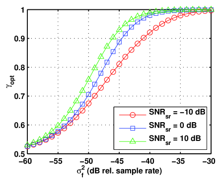
The length of the training signal is and the SNR of the source-destination link is dB (combining the listening and cooperation phases, the effective SNR is dB). The SNR from relay to destination, , is also dB and there is one curve each for . For each curve, the transition from to appears to occur roughly when or . These values of are significant because, for example, when (left half of the plot), the assumed prior knowledge of frequency has more weight than the data, whereas when , the information in the data is more important than the prior model.
IV-E MAP Estimator of and
To calculate the MAP estimate of and at the destination node during the cooperation phase, the covariance between these two random variables (16) is needed. Therefore, the values of and need to be forwarded to the destination node. The log-likelihood of the data at the destination is
| (21) | ||||
where and . As before, choose estimates for and to maximize the likelihood for any given frequency pair,
Substituting these estimates into (IV-E) and minimizing the negative to obtain the MAP frequency estimator
| (22) |
We note the special case of (which implies ). For , the covariance (16) needed in the MAP estimator simplifies to
which has a finite inverse when . However, when , we evaluate the limit of resulting in
where and is the CRB of the frequency in the source-relay link (8) with . The penalty term (last term) of the MAP estimator (IV-E) simplifies to
Thus the penalty term is a quadratic of the frequency difference term normalized by the ratio of error variances (noise power over frequency estimation error variance).
V Simulations
In the previous section, we showed the optimal for extreme values of is either or and when approaches , its effect is small because the frequency adjustment is going toward zero. In this section, we show by simulation, the penalty for choosing instead of is usually limited to a few tenths of a decibel. Thus, near optimal performance is achieved without communicating any of the link SNRs back to the relay for calculation of . We also show the existence of training sequences where (19) is close to (20). Finally, we show the benefit of letting the relay set its transmit frequency based on information received during the listening phase.
We simulate a three node system in a frequency flat environment. In all simulations, we use the SNR of the link (assuming ) as a reference value. The following configuration is considered: let and then vary the link SNR of the source-relay link relative to . Let . The prior distribution for the operating frequency we assume is Gaussian with a variance of dB relative to the sample rate (e.g., a 2 parts-per-million variance of a local oscillator at 900 MHz with 4.5 MHz sample rate [12]).
For flat fading channels and constant modulus training sequences, it is sufficient to choose (the vector of all ones) and . A search is performed to find which minimizes the CRB (19). For values of an exhaustive search over all binary sequences is performed (results hold independent of choice between or ) and for values of , a randomized search over binary sequences is performed. For each value of (up to 128) the optimal sequence for has the following structure:
Sequence Design
Let and
where is length and is the last column of a Sylvester matrix. Then the length optimal sequence is
where is the exchange matrix which reverses the order of elements in the vector it multiplies.
For the configuration described above, and with , Figure 3 shows the difference between the best
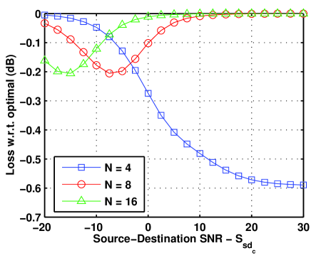
possible CRB (20) (for any constant modulus sequence and ) and the worst case CRB (19) using the binary sequence shown above and . The dB difference for is primarily due to a non-optimal sequence , whereas the dB difference for other values of is due to choosing instead of the optimal value. The loss in performance due to a non-optimal sequence decreases dramatically as increases. These loss values are typical of other system configurations as well. The system behavior as a function of training sequence illustrates the fact that the CRB is insensitive to the selection of these sequences.
Figure 4 shows the sum of the CRB for the two
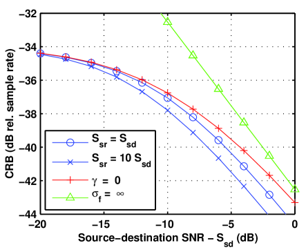
frequencies estimated at the destination node as a function of . For this figure, the SNRs of the source-destination link () and relay-destination link () are the same. The circle and “x”-marks show the CRB when the SNR of the source-relay link is, respectively, the same as and 10 dB higher than . The plus marks show the CRB when . The difference between the plus-marks and the circle and “x”-marks show the potential gain in estimation performance by changing the relay’s transmit frequency (greater benefit when the SNR is large). The triangles show the CRB when no prior information is used. This shows a great advantage of using a prior model when the SNR is low.
VI Sub-Optimal Algorithms
The maximum-likelihood frequency estimator (IV-E) requires a two-dimensional search over the frequency range of interest. As this is a computationally expensive approach to estimation, we compare the mean squared error (MSE) performance of more efficient, sub-optimal estimation algorithms and introduce a correlation based estimator as the best compromise between estimation performance and computational efficiency. In the remainder of this section, we describe the use of the one-dimensional ML algorithm as applied to the two signal case and the correlation algorithm for frequency estimation and compare their performance.
VI-A One-Dimensional ML
As a result of the choice of the training sequence, estimation of the two frequencies is nearly uncoupled. Therefore, performing two independent one-dimensional ML searches for the frequencies is approximately the same as performing the full two-dimensional ML search as required by the ML algorithm. Given the data vector , the one-dimensional ML estimates of the frequencies are
| (23) | ||||
| (24) |
which do not take the correlations between the frequencies into account. To improve the estimates (23) and (24), we assume the variance of each estimate meets the CRB assuming the prior information is uncorrelated for each frequency:
where is a diagonal matrix consisting of the diagonal entries of (zeroing out the other elements). This assumption is valid for high SNR and large . Incorporating this knowledge with the prior information, the least squares estimates of the frequencies are
| (25) |
VI-B Correlation Method
We first describe a standard correlation frequency estimation method as presented in [23] and then provide an extension to allow this algorithm to work in the presence of two signals with known training sequences. Assuming a single signal in the presence of flat fading
The estimated autocorrelation sequence of is
The estimate of the frequency is calculated as
| (26) |
where is a design parameter and the frequency estimate is unambiguous if
Therefore, trades performance for estimation range. The performance of this algorithm (26) is shown in [23] to be close to the CRB when . To ensure adequate estimation range, the maximum allowed value of is 12 (corresponding to a range of five standard deviations away from the mean of the prior). To incorporate the known prior knowledge of the frequency variance, the estimate (26) is adjusted according to the following rule
where is the CRB of the frequency estimate with no prior information. Let
be a function that inputs the data vector , training vector , and prior information, and outputs the frequency estimate according to the above algorithm. This algorithm is used without modification during the listening phase to calculate the estimate .
For the cooperation phase, there are two signals present and the undesired signal acts as interference for the desired signal being estimated. The estimates provided by the correlation algorithm are
| (27) | ||||
| (28) |
which exhibit a floor in MSE (see Figure 5). To improve the estimates, we project out the undesired signal in the following manner:
where the frequency estimates in (27) and (28) are used to calculate the interference signal, which is projected out. The correlation algorithm is run a second time to find
The final frequency estimates, with all prior information accounted for, is calculated similarly to (25),
Figure 5 shows the total MSE
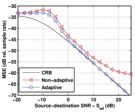
(summation of errors from and ) of the correlation algorithm compared with the CRB for . The triangle markers denote the performance of the algorithm without any adaptation while the circle markers denote the performance of the adaptive two-step algorithm described above. For lower SNRs, the adaptive algorithm has about a 3 dB advantage while the performance difference is much greater at higher SNRs (above 15 dB). The performance of the adaptive algorithm is near optimal. The slight “bump” in performance of the two algorithms at dB SNR is caused by the interaction of the threshold region (the region where the MSE performance breaks away from the CRB) and the region dominated by prior information (where the algorithms converge to a dB MSE relative to the sample rate).
For the same scenario, Figure 6 compares the three
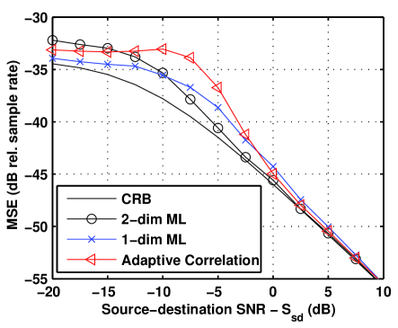
estimation algorithms: full (two-dimensional search) maximum likelihood (circles), one-dimensional ML (“x”-marks), and the adaptive correlation algorithm (triangles). Each of these algorithms approaches the CRB asymptotically in SNR. The differences in behavior at lower SNRs is attributed to the different algorithms entering their threshold regions at different SNRs. A more detailed analysis of this region can be carried out using the methods of [24].
VII Conclusions
In this paper, we have derived the Cramér-Rao bounds for frequency offset estimation in a three-node collaborative communication system. We have shown through simulation, the performance increase obtained by allowing the relay to change its transmitting frequency. We have also shown there exists an optimal transmit frequency for the relay node based on the other link SNRs and the assumed prior knowledge of the frequency offsets. However, there is only a small (tenths of decibels) penalty if the relay always transmits at its estimate of the source frequency. Simulation results also demonstrate the existence of binary training sequences that result in very little loss as compared with an arbitrary constant modulus sequence. We also derived a computationally efficient correlation based estimation algorithm that has mean squared error performance close to the CRB.
References
- [1] P. Mitran, H. Ochiai, and V. Tarokh, “Space-time diversity enhancements using collaborative communications,” IEEE Trans. Inf. Theory, vol. 51, no. 6, pp. 2041–2057, June 2005.
- [2] A. Sendonaris, E. Erkip, and B. Aazhang, “User cooperation diversity – part I: System description,” IEEE Trans. Commun., vol. 51, no. 11, pp. 1927–1938, Nov. 2003.
- [3] ——, “User cooperation diversity – part II: Implementation aspects and performance analysis,” IEEE Trans. Commun., vol. 51, no. 11, pp. 1939–1948, Nov. 2003.
- [4] J. N. Laneman and G. W. Wornell, “Distributed space-time-coded protocols for exploiting cooperative diversity in wireless networks,” IEEE Trans. Inf. Theory, vol. 49, no. 10, pp. 2415–2425, Oct. 2003.
- [5] J. N. Laneman, D. N. C. Tse, and G. W. Wornell, “Cooperative diversity in wireless networks: Efficient protocols and outage behavior,” IEEE Trans. Inf. Theory, vol. 50, no. 12, pp. 3062–3080, Dec. 2004.
- [6] M. Janani, A. Hedayat, T. E. Hunter, and A. Nosratinia, “Coded cooperation in wireless communications: Space-time transmission and iterative decoding,” IEEE Trans. Signal Process., vol. 52, no. 2, pp. 362–371, Feb. 2004.
- [7] G. Foschini and M. Gans, “On limits of wireless communications in a fading environment when using multiple antennas,” Wireless Pers. Commun., pp. 311–335, 1998.
- [8] I. Telatar, “Capacity of multi-antenna Gaussian channels,” Eur. Trans. Telecommun., vol. 10, no. 6, pp. 585–595, Nov./Dec. 1999.
- [9] I. Akyildiz, W. Su, Y. Sankarasubramaniam, and E. Cayirci, “A survey of sensor networks,” IEEE Commun. Mag., vol. 40, no. 8, pp. 102–114, Aug. 2002.
- [10] M. Gastpar and M. Vetterli, “On the capacity of wireless networks: the relay case,” in INFOCOM 2002, vol. 3, 2002, pp. 1577–1586.
- [11] X. Li, “Space-time coded multi-transmission among distributed transmitters without perfect synchronization,” IEEE Signal Process. Lett., vol. 11, no. 12, pp. 948–951, Dec. 2004.
- [12] O. Shin, A. Chan, H. T. Kung, and V. Tarokh, “Design of an OFDM cooperative space-time diversity system,” IEEE Trans. Veh. Technol., to appear.
- [13] J. van de Beek, M. Sandell, and P. O. Börjesson, “Ml estimation of time and frequency offset in OFDM systems,” IEEE Trans. Signal Process., vol. 45, no. 7, pp. 1800–1805, July 1997.
- [14] T. M. Schmidl and D. C. Cox, “Robust frequency and timing synchronization for OFDM,” IEEE Trans. Commun., vol. 45, no. 12, pp. 1613–1621, Dec. 1997.
- [15] M. Morelli and U. Mengali, “Carrier-frequency estimation for transmissions over selective channels,” IEEE Trans. Commun., vol. 48, no. 9, pp. 1580–1589, Sept. 2000.
- [16] O. Besson and P. Stoica, “On parameter estimation of MIMO flat-fading channels with frequency offsets,” IEEE Trans. Signal Process., vol. 51, no. 3, pp. 602–613, Mar. 2003.
- [17] S. Ahmed, S. Lambotharan, A. Jakobsson, and J. A. Chambers, “MIMO frequency-selective channels with multiple frequency offsets: estimation and detection techniques,” IEE Proc. Commun., vol. 152, no. 4, pp. 489–494, Aug. 2005.
- [18] P. A. Parker, P. Mitran, D. W. Bliss, and V. Tarokh, “Adaptive frequency synchronization for collaborative communication systems,” in Int. Conf. on Distributed Computing Systems (ICDCS), Toronto, Canada, June 2007.
- [19] H. L. V. Trees, Detection, Estimation, and Modulation Theory: Part 1. Wiley Interscience, 1968.
- [20] S. T. Smith, “Statistical resolution limits and the complexified Cramér-Rao bound,” IEEE Trans. Signal Process., vol. 53, no. 5, pp. 1597–1609, May 2005.
- [21] T. K. Moon and W. C. Stirling, Mathematical Methods and Algorithms for Signal Processing. Prentice Hall, 2000.
- [22] L. L. Scharf, Statistical Signal Processing: Detection, Estimation, and Time Series Analysis. Addison Wesley, 1991.
- [23] M. Luise and R. Reggiannini, “Carrier frequency recovery in all-digital modems for burst-mode transmissions,” IEEE Trans. Commun., vol. 43, no. 2/3/4, pp. 1169–1178, Feb./Mar./Apr. 1995.
- [24] C. D. Richmond, “Mean-squared error and threshold SNR prediction of maximum-likelihood signal parameter estimation with estimated colored noise covariances,” IEEE Trans. Inf. Theory, vol. 52, no. 5, pp. 2146–2164, May 2006.