CMB and LSS constraints on a single-field model of inflation

Abstract

A new inflationary scenario whose exponential potential $V(\Phi)$ has a quadratic dependence on the field $\Phi$ in addition to the standard linear term is confronted with the tree-year observations of the Wilkinson-Microwave Anisotropy Probe and the Sloan Digital Sky Survey data. The number of e-folds ($N$), the ratio of tensor-to-scalar perturbations ($r$), the spectral scalar index of the primordial power spectrum ($n_{s}$) and its running ($dn_{s}/d\ln k$) depend on the dimensionless parameter $\alpha$ multiplying the quadratic term in the potential. In the limit $\alpha\rightarrow 0$ all the results of the standard exponential potential are fully recovered. For values of $\alpha\neq 0$, we find that the model predictions are in good agreement with the current observations of the Cosmic Microwave Background (CMB) anisotropies and Large-Scale Structure (LSS) in the Universe.

I Introduction

Since the detection of the Cosmic Microwave Background (CMB) anisotropies by the COBE satellite in 1992 cobe , great improvements in the quality of the CMB data has been achieved, mainly from very recent baloon and satellite experiments, such as the BOOMERANG boomerang and the Wilkinson Microwave Anisotropy Probe (WMAP) wmap ; wmap3 . In what concerns the possible implications on the inflationary epoch, for instance, the current three-year WMAP (WMAP3) data seemed, at a first moment, to have precision enough to discriminate between some single-field inflationary models. In fact, soon after the WMAP3 data release, some authors arrived to the conclusion that quartic chaotic inflationary scenarios of the form $V(\Phi)\sim\lambda\Phi^{4}$ were ruled out, while quadratic chaotic inflationary models with potential, $V(\Phi)\sim m^{2}\Phi^{2}$, agreed only marginally with the observational data wmap3 ; easther ; lyth . The original WMAP3 parameter-estimation analysis also pointed to a spectral index smaller ($n_{s}\simeq 0.95$) than the Zel’dovich spectrum of density perturbations, for which adiabatic perturbations have a scale-invariant spectral index ($n_{s}=1$). Although compatible with some theoretical predictions mukanov , the latter conclusion was rediscussed by a recent analysis of the WMAP3 data from a more sophisticated statistical approach of model selection and systematic effects, leading to values of $n_{s}$ still compatible with the Zel’dovich prediction melchi .

The WMAP3 data also place an upper limit on the tensor-to-scalar ratio, i.e., $r<0.55$ (at 95.4% c.l.), whereas a joint analysis involving the WMAP3 data and the large-scale power spectrum of luminous red galaxies in the Sloan Digital Sky Survey (SDSS) provides $r<0.33$ (also at 95.4% c.l.) tegmark . In light of all these observational results, a number of authors have tested the viability of different types of inflationary models (see, e.g., easther ; lyth ; scenarios ; beta ; b1 ). As an example, very recently, the authors of Ref. b1 revived a interesting phenomenological model with a simple slowly-rolling scalar field that, in the light of the WMAP3 data, does not present a pure de Sitter inflationary expansion, but produce a Zel’dovich spectrum, i.e., $n_{s}=1$.

Given the current availability of high precision cosmological data and, as consequence, the real possibility of truly ruling out some theoretical scenarios, it is timely to revive old inflationary models (as done in Ref. b1 ), as well as to investigate new ones. In this paper, motivated by a transient dark energy scenario recently proposed in Ref. prl , we study a single, minimally-coupled scalar field model of inflation whose evolution is described by an exponential potential $V(\Phi)$ that has a quadratic dependence on the field $\Phi$ in addition to the standard linear term. Such a potential is obtained through a simple ansatz and fully reproduces the Ratra-Peebles scenario studied in Ref. exp (see also r1 ; r2 ) in the limit of the dimensionless parameter $\alpha\rightarrow 0$. For all values of $\alpha\neq 0$, however, the potential is dominated by the quadratic contribution and admits a wider range of solutions than do conventional exponential potentials.

In this context, our aim here is to test the viability of this new class of inflationary scenario in light of the current CMB and LSS data. In Sec. II we deduce the inflaton potential $V(\Phi)$ and discuss the basic features of the model. The slow-roll inflation driven by this potential along with some important observational quantities, such as the spectral index, its running, and the ratio of tensor-to-scalar perturbations, are discussed in Sec. III. We also confront our theoretical results with the most recent CMB and LSS observations, as analized in Refs. wmap3 ; tegmark ; melchi . Finally, the main results of this paper are discussed and summarized in the Sec. IV.

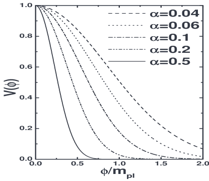
Figure 1: The potential $V(\Phi)$ as a function of the field [Eq. (6)] for some selected values of the parameter $\alpha$.

II Single-field model

In what follows we assume that the Universe is nearly flat, as evidenced by the combination of the position of the first acoustic peak of the CMB power spectrum and the current value of the Hubble parameter wmap3 . To begin with, let us consider a single scalar field model whose action is given by

$$S=\frac{m^{2}_{\rm pl}}{16\pi}\int d^{4}x\sqrt{-g}\left[R-\frac{1}{2}\partial^{\mu}\Phi\partial_{\mu}\Phi-V(\Phi)\right]\;.$$ (1)

In the above expression, $m_{\rm pl}\equiv G^{-1/2}\approx 10^{19}GeV$ is the Planck mass and we have set the speed of light $c=1$.

For an inflaton-dominated universe, the Friedmann equation is written as

$$H^{2}=\left(\frac{\dot{a}}{a}\right)^{2}=\frac{8\pi}{3m_{\rm pl}^{2}}\left[\frac{1}{2}\dot{\Phi}^{2}+V\left(\Phi\right)\right]\;,$$ (2)

where $a(t)$ is the cosmological scalar factor and dots denote derivatives with respect to time. By combining Eq. (2) with the conservation equation for the $\Phi$ component, i.e., $\dot{\rho}_{\Phi}+3H(\rho_{\Phi}+p_{\Phi})=0$, we obtain

$$\frac{\partial\Phi}{\partial a}=\sqrt{-\frac{m_{\rm pl}^{2}}{8\pi a}\frac{1}{\rho_{\Phi}}\frac{\partial\rho_{\Phi}}{\partial a}}\;,$$ (3)

where $\rho_{\Phi}=\frac{1}{2}\dot{\Phi}^{2}+V(\Phi)$ and $p_{\Phi}=\frac{1}{2}\dot{\Phi}^{2}-V(\Phi)$ are, respectively, the inflaton energy density and pressure.

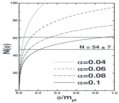
Figure 2: The predicted number of e-folds $N(\Phi)$ as a function of the field for some selected values of the parameter $\alpha$. The horizontal lines correspond to 1$\sigma$ limit on the number of e-folds ($N=54\pm 7$) discussed in Ref. e-fold .

Following Ref. prl , we adopt an ansatz on the scale factor derivative of the energy density, i.e.,

$$\frac{1}{\rho_{\Phi}}\frac{\partial\rho_{\Phi}}{\partial a}=-\frac{\lambda}{a^{1-2\alpha}}\;,$$ (4)

where $\alpha$ and $\lambda$ are positive parameters, and the factor 2 was introduced for mathematical convenience. From a direct combination of Eqs. (3) and (4), the following expression for the scalar field is obtained

$$\Phi(a)=\frac{1}{\sqrt{\sigma}}\ln_{1-\alpha}\left({a}\right)\;,$$ (5)

where $\sigma={8\pi/\lambda m_{\rm pl}^{2}}$ and the generalized logarithmic function $\ln_{1-\xi}$, defined as $\ln_{1-\xi}(x)\equiv{(x^{\xi}-1)/\xi}$, reduces to the ordinary logarithmic function in the limit $\xi\rightarrow 0$ abramowitz . The potential $V(\Phi)$ for the above scenario is easily derived by using the definitions of $\rho_{\Phi}$ and $p_{\Phi}$ and inverting Eq. (5), i.e.,

$$V(\Phi)=f(\alpha;\Phi)\exp\left[-\lambda\sqrt{\sigma}\left(\Phi+\frac{\alpha\sqrt{\sigma}}{2}\Phi^{2}\right)\right],$$ (6)

where $f(\alpha;{\Phi})\propto[1-\frac{\lambda}{6}(1+\alpha\sqrt{\sigma}{\Phi})^{2}]$. The most important aspect to be emphasized at this point is that in the limit $\alpha\rightarrow 0$ Eqs. (5) and (6) fully reproduce the exponential potential studied by Ratra and Peebles in Ref. exp , while $\forall$ $\alpha\neq 0$ the scenario described above represents a generalized model which admits a wider range of solutions. This means that all the physical observational quantities derived in the next section have the ordinary exponential case as a particular limit when $\alpha\rightarrow 0$. For the sake of completeness, in Fig.(1) we show the potential $V(\Phi)$ as a function of the field for several values of the parameter $\alpha$ and a fixed value of $\lambda=10^{-6}$ (see prl for details).

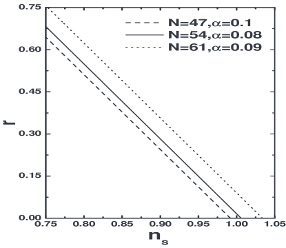
Figure 3: The $n_{s}-r$ plane for some selected values of the parameter $\alpha$ to first-order in slow-roll approximation. Note that, similarly to the intermediate inflationary model of Ref. b1 , it is possible to obtain a scale-invariant spectrum for nonvanishing values of $r$.

III Slow-roll Inflation

III.1 Slow-roll Parameters

In this background, the energy conservation law for the field can be expressed as $\ddot{\Phi}+3H\dot{\Phi}+V^{\prime}\left(\Phi\right)=0$, where primes denote derivative with respect to the field $\Phi$. In the so-called slow-roll approximation, the evolution of the field is dominated by the drag from the cosmological expansion, so that $\ddot{\Phi}\approx 0$ or, equivalently, $3H\dot{\Phi}+V^{\prime}\simeq 0$. With these simplifications, the slow-roll regime can be expressed in terms of the slow-roll parameters $\epsilon$ and $\eta$, i.e., book ; lyth1

$$\epsilon=\frac{m^{2}_{\rm pl}}{16\pi}\left(\frac{V^{\prime}}{V}\right)^{2}=\frac{\lambda}{2}\frac{[\lambda y^{2}-2(\alpha+3)]^{2}y^{2}}{(6-\lambda y^{2})^{2}}\;,$$ (7)

and

$$\eta=\frac{m^{2}_{\rm pl}}{8\pi}\frac{V^{\prime\prime}}{V}=\frac{(5\alpha+6)\lambda y^{2}-\lambda^{2}y^{4}-2\alpha(\alpha+3)}{6-\lambda y^{2}}\;,$$ (8)

where, for the sake of simplicity, we have introduced the variable $y=1+\alpha\sqrt{\sigma}\Phi$. Note that, in the limit $\alpha\rightarrow 0$, the above expressions reduce, respectively, to $\epsilon_{\alpha\rightarrow 0}=\frac{\lambda}{2}$ and $\eta_{\alpha\rightarrow 0}=\lambda$, as expected from conventional exponential potentials.

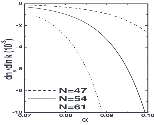
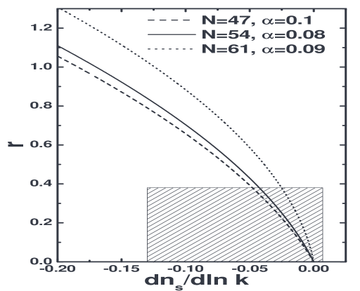
Figure 4: a) The $\alpha-dn_{s}/d\ln k$ plane for the number of e-folds lying in the interval $N=54\pm 7$. Note that, as $\alpha\rightarrow 0$, $dn_{s}/d\ln k$ also $\rightarrow 0$, as expected from exponential potentials. The same conclusion on $dn_{s}/d\ln k$ also persists for negative values of the index $\alpha$. b) The $dn_{s}/d\ln k-r$ plane for $\alpha=0.1,0.09$ and 0.08. Here, the hachured region corresponds to $-0.13\leq dn_{s}/d\ln k\leq 0.007$ and $r<0.38$ (at 95.4%), as given in Ref. melchi .

For the above scenario, we can also compute the predicted number of e-folds by using Eq. (5) and (7), i.e., $N=\int Hdt=\ln\left[1+\alpha\sqrt{\sigma}\Phi_{N}\right]^{1/\alpha}$, which reduces, in the limit $\alpha\rightarrow 0$, to $N_{\alpha\rightarrow 0}\propto\Phi_{\rm N}$. The result of this calculation is shown in Fig. (2) as the $N-\Phi$ plane for some selected values of the index $\alpha$. The horizontal lines in the figure correspond to the 1$\sigma$ bound on the number of e-folds discussed in Ref. lyth , i.e., $N=54\pm 7$. To test the viability of the inflationary scenario here discussed, in all the subsequent analyses we follow Ref. lyth and adopt the interval $N=54\pm 7$. Without loss of generality, we also fix the value of the constant $\lambda$ at $\simeq 10^{-6}$.

III.2 Spectral Index

In order to confront our model with current observational results we first consider the spectral index, $n_{s}$, and the ratio of tensor-to-scalar perturbations, $r$. In terms of the slow-roll parameters to first order, these quantities, defined as $n_{s}-1=2\eta-6\epsilon$ and $r=16\epsilon$, are now expressed as

$$n_{s}-1=-\frac{[\lambda y^{2}-2(\alpha+3)]^{2}y^{2}}{(6-\lambda y^{2})^{2}}[3\lambda+2(6-\lambda y^{2})]+\frac{2\lambda y^{2}(\alpha-6)+4(\alpha+3)(\alpha+6)}{6-\lambda y^{2}},$$ (9)

and

$$r=8\lambda\frac{[\lambda y^{2}-2(\alpha+3)]^{2}y^{2}}{(6-\lambda y^{2})^{2}}\;.$$ (10)

As can be easily verified, in the limit $\alpha\rightarrow 0$, the above expressions reduce, respectively, to $(n_{s}-1)_{\alpha\rightarrow 0}=-\lambda$ and $r_{\alpha\rightarrow 0}=8\lambda$. For $r<0.55$ (95.4% c.l.), as given by current CMB data wmap3 , one obtains from Eq. (10) $\epsilon<0.03$, which is in agreement with the slow-roll approximation discussed earlier and adopted in our analysis.

Figure (3) shows the $n_{s}-r$ plane, given by

$$r=\frac{8}{\gamma-3}(n_{s}-1)\;,$$ (11)

where

$$\gamma=\frac{2(\lambda y^{2}-6)}{\lambda y^{2}}\left[1-\frac{\lambda y^{2}(\alpha-6)+2(\alpha+3)(\alpha+6)}{(\lambda y^{2}-2\alpha-6)^{2}}\right],$$ (12)

for some selected values of $\alpha$. Note that, in the limit $\alpha\rightarrow 0$ or, equivalently, $\gamma\rightarrow 2$, Eq. (11) reduces to $r_{\alpha=0}=8(1-n_{s})$, as predicted by exponential models melchi . Also, and very important, we note from this figure that, for these selected values of the parameter $\alpha$, the inflationary scenario discussed in this paper seems to be in agreement with current observational data from CMB and LSS measurements. As a first example, let us take the tensor fraction $r$ to be negligible. In this case, the analyses involving WMAP3 plus SDSS and WMAP3 plus 2dFGRS data provide, respectively, $n_{s}=0.980\pm 0.020$ and $n_{s}=0.956\pm 0.020$ (68.3% c.l.), which are clearly in agreement with the model predictions (at $2\sigma$ level) shown in Fig. (3), i.e., $n_{s}\simeq 1.03$ ($N=47$), $n_{s}\simeq 1.01$ ($N=54$), and $n_{s}\simeq 0.97$ ($N=61$). Similar conclusions can also be obtained by considering $r\neq 0$. In this case, the current data from WMAP3 plus SDSS provides a tensor fraction $r<0.33$ and $n=0.980\pm 0.020$, while the model discussed in this paper predicts for this interval of $r$, $n_{s}\geq 0.95$ ($N=47$), $n_{s}\geq 0.92$ ($N=54$), and $n_{s}\geq 0.88$ ($N=61$). From this figure, it is also possible to obtain a scale-invariant spectrum ($n_{s}=1$) for values of $r\neq 0$, as discussed in the context of the intermediate inflationary model of Ref. b1 .

III.3 Running of the Spectral Index

The running of the spectral index in the inflationary regime, to lowest order in the slow-roll approximation, is given by running

$$\frac{dn_{s}}{d\ln k}=-2\xi^{2}+16\epsilon\eta-24\epsilon^{2}$$ (13)

where $\epsilon$ and $\eta$ are, respectively, the first and the second slow-roll parameters, defined in Eqs. (7) and (8). Here, $\xi^{2}$ is the third slow-roll parameter, which is related with the third derivative of the potential by

$$\xi^{2} = \frac{m_{\rm pl}^{2}}{64\pi^{2}}\frac{V^{\prime\prime\prime}V^{\prime}}{V^{2}}=\lambda\frac{[6\alpha(2\alpha+3)-3(\alpha+2)\lambda y^{2}+\lambda^{2}y^{4}][\lambda y^{2}-2(\alpha+3)]y^{2}}{(6-\lambda y^{2})^{2}}\;.$$ (14)

Note that in the limit $\alpha\rightarrow 0$, the $\xi$ parameter reduces to $\xi^{2}_{\alpha\rightarrow 0}=\lambda^{2}$ and, as expected for usual exponential potentials, the running, expressed by Eq. (13), vanishes.

This and other features of the inflationary scenario discussed in this paper are shown in Figs. (4a) and (4b). In Fig. (4a) the $\alpha-dn_{s}/d\ln k$ plane is displayed for values of the number of e-folds lying in the interval $N=54\pm 7$. Note that, differentlty from other models discussed in the literature (see, e.g. beta ), this scenario predicts only positive values for the running of the spectral index, which seems to be in full agreement with the WMAP3 data ($-0.17\leq dn_{s}/d\ln k\leq-0.02$ at $95.4\%$ c.l.) but only partially compatible with the joint analysis involving WMAP3 and SDSS data ($-0.13\leq dn_{s}/d\ln k\leq 0.007$ at $95.4\%$) of Ref. melchi . In Fig. (4b) we show the $dn_{s}/d\ln k-r$ plane for $\alpha=0.1,0.09$ and $0.08$. Here, the shadowed region corresponds to the 95.4% limit on the ratio of tensor-to-scalar pertubations, i.e., $r<0.38$ melchi . As can be seen from this Panel, for two out of the three combinations of the pair $\alpha-N$, the model predictions agree reasonably well with the current bounds from CMB and LSS data.

IV Final remarks

Primordial inflation inflation1 constitutes one of the best and most successful examples of physics at the interface between particle physics and cosmology, with tremendous consequences on our view and understanding of the observable Universe (see, e.g., revInf ; book ; lyth1 for review). Besides being the current favorite paradigm for explaining both the causal origin of structure formation and the Cosmic Microwave Background (CMB) anisotropies, an inflationary epoch in the very early Universe also provides a natural explanation of why the Universe is nearly flat ($\Omega_{k}\simeq 0$), as evidenced by the combination of the position of the first acoustic peak of the CMB power spectrum and the current value of the Hubble parameter wmap3 .

In this work, we have discussed cosmological implications of the single, minimally-coupled scalar field model recently proposed in Ref. prl , whose evolution is described by an exponential potential $V(\Phi)$ that has a quadratic dependence on the field $\Phi$ in addition to the standard linear term. As discussed in Sec. II, this potential fully reproduces the Ratra-Peebles inflation studied in Ref. exp in the limit of the dimensionless parameter $\alpha\rightarrow 0$. We have calculated the main observable quantities in the slow-roll regime and shown that, even for values of the number of e-folds in the restrictive interval $N=54\pm 7$ lyth , the predictions of the model for values of $\alpha\neq 0$ seem to be in good agreement with current bounds on these parameters from CMB and LSS observations, as given in Refs. melchi ; tegmark . Similarly to the intermediate inflationary scenario discussed in Ref. b1 , it is also possible to obtain a scale-invariant spectrum $(n_{s}=1)$ for vanishing values of the tensor-to-scalar ratio $r$. For values of $r\simeq 0$ or, equivalently, $n_{s}\simeq 1$, we have found that the theoretical prediction for the running of the spectral index approaches to zero from negative values, which is compatible with current observations from CMB data, i.e., $-0.17\leq dn_{s}/d\ln k\leq-0.02$ (at $95.4\%$ c.l.) wmap3 .

This work is partially supported by the Conselho Nacional de Desenvolvimento Científico e Tecnológico (CNPq - Brazil). JSA is also supported by FAPERJ No. E-26/171.251/2004 and JASL by FAPESP No. 04/13668-0.

References

- (1) G. F. Smoot et al., Astrophys. J. 396, L1 (1992).
- (2) P. de Bernardis et al., Nature 404, 955 (2000); C. J. MacTavish et al., Astrophys. J. 647, 799 (2006).
- (3) D. N. Spergel et al., Astrophys. J. Suppl. 148, 175 (2003).
- (4) D. N. Spergel et al., arXiv:astro-ph/0603449
- (5) L. Alabidi and D. H. Lyth, JCAP 0605, 016 (2006); L. Alabidi and D. H. Lyth, JCAP 0608 013 (2006).
- (6) R. Easther and H. Peiris, JCAP 0609 (2006) 010; H. Peiris and R. Easther, JCAP 0610 (2006) 017.
- (7) V. F. Mukhanov and G. V. Chibisov, JETP Lett. 33 (1981) 532, Pisma Zh. Eksp. Teor. Fiz. 33 (1981) 549.
- (8) W. H. Kinney, E. W. Kolb, A. Melchiorri and A. Riotto, Phys. Rev. D 74, 023502 (2006).
- (9) M. Tegmark et al., Phys. Rev. D 74, 123507 (2006).
- (10) R. Opher and A. Pelinson, Braz. J. Phys. 36, 566 (2006); R. Rosenfeld and J. A. Frieman, Phys. Rev. D75, 043513 (2007).
- (11) J.S. Alcaniz and F.C. Carvalho, arXiv: astro-ph/0612279.
- (12) J. D. Barrow, A. R. Liddle and C. Pahud, Phys. Rev. D 74, 127305 (2006)..
- (13) F. C. Carvalho, J. S. Alcaniz, J. A. S. Lima and R. Silva, Phys. Rev. Lett. 97, 081301 (2006), arXiv:astro-ph/0608439.
- (14) P. J. E. Peebles and B. Ratra, Astrophys. J. Lett. 325, L17 (1988); B. Ratra and P. J. E. Peebles, Phys. Rev D37, 3406 (1988)
- (15) C. Wetterich, Astron. & Astrophys. 301, 321 (1995)
- (16) P. G. Ferreira and M. Joyce, Phys. Rev. D58, 023503(1998).
- (17) M. Abramowitz and I. Stegun, Handbook of Mathematical Functions, Dover, New York, (1965). See also J.A.S. Lima, R. Silva and A.R. Plastino, Phys. Rev. Lett., 86, 2938 (2001).
- (18) S. Dodelson and L. Hui, Phys. Rev. Lett. 91, 131301 (2003); A. R. Liddle and S. M. Leach, Phys. Rev. D68, 103503 (2003).
- (19) B. A. Bassett, S. Tsujikawa and D. Wands, Rev. Mod. Phys. 78, 537 (2006); G. Ballesteros, J. A. Casas and J. R. Espinosa, JCAP 0603, 001 (2006).
- (20) A. A. Starobinsky, Phys. Lett. B91, 99 (1980); A. H. Guth, Phys. Rev. D 23 (1981) 347; A. D. Linde, Phys. Lett. B 116, 335 (1982); A. Albrecht and P. J. Steinhardt, Phys. Rev. Lett. 48,1220 (1982)
- (21) R. H. Brandenberger, Braz. J. Phys. 31,131 (2001); J. E. Lidsey et al., Rev. Mod. Phys. 69, 373 (1997); A. Linde, New Astronomy Review, 49, 35 (2005).
- (22) A. R. Liddle and D. H. Lyth, Cosmological Inflation and Large-Scale Structure, CUP, Cambridge, 2000.
- (23) D. H. Lyth and A. Riotto, Phys. Rept. 314, 1 (1999).