Impact of dimensionless numbers on the efficiency of MRI-induced turbulent transport.

Abstract

The magneto-rotational instability is presently the most promising source of turbulent transport in accretion disks. However, some important issues still need to be addressed to quantify the role of MRI in disks; in particular no systematic investigation of the role of the physical dimensionless parameters of the problem on the dimensionless transport has been undertaken yet. For completeness, we first generalize existing results on the marginal stability limit in presence of both viscous and resistive dissipation, exhibit simple scalings for all relevant limits, and give them a physical interpretation. We then reexamine the question of transport efficiency through numerical simulations in the simplest setting of a local, unstratified shearing box, with the help of a pseudo spectral incompressible 3D code; viscosity and resistivity are explicitly accounted for. We focus on the effect of the dimensionless magnetic field strength, the Reynolds number, and the magnetic Prandtl number. First, we complete existing investigations on the field strength dependence by showing that the transport in high magnetic pressure disks close to marginal stability is highly time-dependent and surprisingly efficient. Second, we bring to light a significant dependence of the global transport on the magnetic Prandtl number, with $\alpha\propto Pm^{\delta}$ for the explored range: $0.12<Pm<8$ and $200<Re<6400$ ($\delta$ being in the range 0.25 to 0.5). We show that the dimensionless transport is not correlated to the dimensionless linear growth rate, contrarily to a largely held expectation. For large enough Reynolds numbers, one would expect the reported Prandtl number scaling of the transport should saturate, but such a saturation is out of reach of the present generation of supercomputers. Understanding this saturation process is nevertheless quite critical to accretion disk transport theory, as the magnetic Prandtl number $Pm$ is expected to vary by many orders of magnitude between the various classes of disks, from $Pm\ll 1$ in YSO disks to $Pm\gtrsim$ or $\gg 1$ in AGN disks. More generally, these results stress the need to control dissipation processes in astrophysical simulations.

1 Introduction

Angular momentum transport has always been a central issue in accretion disk theory. The first $\alpha$ model (Shakura & Sunyaev, 1973) already assumed the presence of strong turbulent motions, modelled through an effective viscosity, orders of magnitude larger than the expected disk molecular viscosity. Since then, the physical origin of this turbulence has been highly debated. As purely hydrodynamic non stratified Keplerian flows are known to be linearly stable to small perturbations, a finite amplitude instability was first envisioned to trigger turbulence. This question was studied both experimentally (Richard & Zahn, 1999; Richard, 2001; Richard et al., 2001) and numerically (Balbus et al., 1996; Hawley et al., 1999), leading to a long controversy. More recent numerical and experimental investigations of this problem strongly support the idea that the transport due to this mechanism, if present, would be far to inefficient to account for the short disk evolution time-scales imposed by astrophysical observations (Lesur & Longaretti, 2005; Ji et al., 2006). Linear instabilities of hydrodynamic origin have also been envisioned as a source of turbulence, relating in particular to the flow stratification (Klahr & Bodenheimer, 2003; Urpin, 2003; Dubrulle et al., 2005; Shalybkov & Ruediger, 2005), but these are either not present or too inefficient (Johnson & Gammie 2006; Arlt & Urpin 2004; Longaretti & Lesur 2007; see Lesur & Longaretti 2005 and references therein for a recent review of this issue).

The potential role of MHD instabilities in accretion disks was pointed out in a seminal paper by Balbus & Hawley (1991), devoted to an analysis of what is now known as the magneto-rotational instability (MRI). This instability has extensively been studied since then, mainly with the help of local (Hawley et al., 1995; Stone et al., 1996) and global (Hawley, 2000) 3D numerical simulations. Although a more recent set of numerical simulations did focus on MRI energetics (Gardiner & Stone, 2005), the dissipation of turbulent fields in these simulations is not controlled, as no physical term was introduced to account for physical viscosity and resistivity. Note however that Brandenburg et al. (1995) have introduced such dissipation in their simulations, but kept it as small as possible, and in any case did not try to investigate their effect in a systematic way. Resistivity effects alone have also been introduced by Fleming et al. (2000), but viscous effects were still neglected. This raises questions about the exact role of numerical dissipation in all these simulations, especially at the light of our recent investigation of subcritical turbulence in accretion disks (Lesur & Longaretti, 2005), which clearly showed that a careful control of dissipation and resolution — and more generally of the dimensionless parameters of the problem — is required to properly quantify turbulent transport.

This issue is addressed here in the context of MRI-driven turbulence, using a 3D spectral Fourier code, which allows a precise monitoring of viscous, resistive and numerical dissipation. First, we recall the MHD equations in the shearing sheet framework (Hawley et al., 1995), along with the relevant dimensionless parameters of the problem, and summarize what is known about their effect on MRI-induced turbulent transport. Next, we investigate the linear stability of the MRI, which to the best of our knowledge has not been fully characterized when both viscosity and resistivity are accounted for in the dispersion relation. Then, we present new results on the behavior of turbulent transport in dimensionless parameters regime that have not been investigated in the past: first, very close to the threshold of instability (in terms of relative magnetic field strength), and then with respect to the magnetic Prandtl number, which has been ignored in all previous investigations. The dependence of turbulence transport on the magnetic Prandtl number is the most significant finding of this investigation. This dependence may turn out to be critical, as the magnetic Prandtl number varies by many order of magnitudes in astrophysical disks. The astrophysical implications of our findings are further discussed in our concluding section, along with potential caveats relating to numerical limitations that may influence our results.

2 Shearing box characterization and summary of earlier results

The MRI has already been extensively studied in the literature (see, e.g., Balbus 2003 and references therein for a review of the subject). Our objective is to extend previous work through a systematic exploration of the dependence of the MRI-induced transport on the physical quantities characterizing the problem. For simplicity, we work in a shearing sheet setting (see Hawley et al. 1995 for a description of the shearing box equations, numerical boundary conditions, and conserved quantities); vertical stratification is ignored, but both viscous and resistive microphysical (molecular) dissipation are included. This differs from previous investigations, where this is always ignored. Our previous experience with subcritical hydrodynamic transport has shown us that the inclusion of explicit dissipation is required to precisely characterize transport properties and ro sort out converged simulations from under-resolved ones (see Lesur & Longaretti 2005 for an extensive discussion and illustration of these points).

The problem is formulated in a cartesian frame centered at $r=R_{0}$, rotating with the disk at $\Omega=\Omega(R_{0})$ with radial dimension $H\ll R_{0}$. In this work, $H$ is the size of our simulation boxes, in the vertical and radial dimensions. This leads to the following set of equation, assuming $\phi\to x$, $r\to-y$:

$$\partial_{t}\bm{u}+\bm{u}\cdot\bm{\nabla}\bm{u} = -\frac{1}{\rho}\bm{\nabla}P+\frac{1}{\mu_{0}\rho}(\bm{\nabla}\times\bm{B})\times\bm{B},$$

$$-2\bm{\Omega}\times\bm{u}-2\Omega Sy\bm{e_{y}}+\nu\bm{\Delta}\bm{u}$$

$$\partial_{t}\bm{B} = \bm{\nabla}\times(\bm{u}\times\bm{B})+\eta\bm{\Delta{B}},$$ (2)

$$\nabla\cdot\bm{u} = 0,$$ (3)

$$\nabla\cdot\bm{B} = 0,$$ (4)

where the medium is defined by $S=-r\partial_{r}\Omega$. For simplicity, incompressible motions are assumed. This is a priori justified by the fact that MRI-induced motions are usually subsonic, so that one expects at least in first approximation that compressibility effects do not play a major role in the problem. This approximation allows us to remove the flow Mach number from the list of dimensionless parameters characterizing the problem, so that we can more effectively isolate and quantify the role of the various physical agents.

The terms on the right-hand side member of Eq. (2) are the gas pressure, Lorentz force, Coriolis force, tidal force, and viscous dissipation, respectively. The steady-state solution to this equation is the local profile $\bm{u}=Sy\bm{e_{x}}$ with $S=3/2\Omega$ for Keplerian disks. In the remainder of this paper, we will use the deviation from the laminar profile $\bm{w}$ defined by $\bm{w}=\bm{u}-Sy\bm{e_{x}}$. For simplicity, we assume that the steady-state magnetic field $B_{0}$ lies along the vertical axis. Note that this field is also the average field in the shearing sheet box, and is conserved during the evolution thanks to the shearing sheet boundary conditions (Hawley et al., 1995).

These equations are characterized by four dimensionless numbers, the first three relating to the Navier-Stokes equation while the last one belongs to the induction equation:

• The Reynolds number, $Re\equiv SH^{2}/\nu$, measuring the relative importance of nonlinear coupling through the advection term, and viscous dissipation.

• A proxy to the plasma beta parameter, defined here as $\beta=S^{2}H^{2}/V_{A}^{2}$ where $V_{A}^{2}=B_{o}^{2}/\mu_{o}\rho$ is the Alfvén speed. The rationale of this definition follows from the vertical hydrostatic equilibrium constraint $c_{s}\sim\Omega H$, which is expected to hold in thin disks, so that our definition of $\beta$ is indeed related to the plasma parameter in an equivalent, vertically stratified disk. This parameter measures the relative weight of the Lorentz force and the advection term.

• The rotation number (inverse Rossby number), defined as $R_{\Omega}=2\Omega/S$, which measures the relative importance of the Coriolis force.

• The magnetic Reynolds number, $R_{m}=SH^{2}/\eta$, which measures the relative importance of resistive dissipation with respect to the ideal term in the induction equation.

We consider only Keplerian disks in this investigation, so that the rotation number is held fixed to its Keplerian value $R_{\Omega}=-4/3$. This leaves us with three independent dimensionless numbers: $\beta$, $Re$, and $Rm$.

On the other hand, the (local in the disk) dimensionless transport coefficient,

$$\alpha=\frac{\langle v_{x}v_{y}-B_{x}B_{y}/(\mu_{o}\rho)\rangle}{S^{2}H^{2}},$$ (5)

being a dimensionless number, can only depend on the local dimensionless parameters characterizing the flow that we have just defined (the bracketing refers to appropriate box and/or time averages). Our task reduces to characterize this dimensionless transport, as a function of the three independent dimensionless numbers just defined. However, for later convenience, we take them to be $\beta$, $Re$ and $P_{m}\equiv\nu/\eta=Rm/Re$ instead (the rationale of this latter choice will become apparent later on).

All previous investigations ignore the dependence on the last two dimensionless numbers, who have not been included in the physical description up to now. Within such an approximation, Hawley et al. (1995) have characterized the dependence of $\alpha$ on $\beta$. Their results imply that

$$\alpha\simeq 3\beta^{-1/2},$$ (6)

from their Eqs. (10), (15), (16) and (18).

This implies in particular that $\alpha$ increases when the initial (and box average) magnetic field $B_{o}$ is increased. However, for a large enough field, the smallest unstable wavelength (which increases along with $B_{o}$) becomes larger than the box size, and the instability is quenched. On this basis, one expects that the scaling Eq. (6) would break down close enough to the critical $\beta$ stability limit. This question is somewhat investigated in the present work. However, most of our effort is devoted to characterizing the $Re$ and $Pm$ dependence of $\alpha$.

3 Linear stability analysis

In order to quantify the MRI induced turbulent transport, it is first necessary to define the parameter domain in which this instability operates. The linear stability of differentially rotating disks in presence of a magnetic field was first investigated in the astrophysical context by Balbus & Hawley (1991). Then, the instability in the weakly ionized case has been considered (Blaes & Balbus, 1994; Wardle, 1999; Balbus & Terquem, 2001), leading to the well known Dead Zone problem (Gammie, 1996). However, we are not aware of any reasonably complete and heuristically clarified investigation of the stability limits of the fluid when both viscous and resistive dissipation are taken into account. Some discussions of this point are available in the literature, mostly motivated by liquid-metal experiments, in the limit $Pm\ll 1$ (Ji et al., 2001; Rüdiger & Shalybkov, 2002). However, these papers exhibit no clear asymptotical limit that may be useful for astrophysical disks. Therefore, we provide such an analysis here, as a prelude to our nonlinear simulations.

We will consider only axisymmetric perturbations, so that we can eliminate the azimuthal perturbation transport term. Note that this assumption does not seem to have a great influence on the stability limit, since 3D numerical simulations and linear analysis of axisymmetric modes exhibit nearly the same stability limit; this holds in particular in the simulations presented here.

We linearize and Fourier transform the equations of motion by assuming $\bm{v}=\bm{v_{0}}\exp\big{(}i(\omega t-k_{y}y-k_{z}z)\big{)}$ and $\bm{b}=\bm{b_{0}}\exp\big{(}i(\omega t-k_{y}y-k_{z}z)\big{)}$. This yields the following linearized equation set:

$$(i\omega+\nu k^{2})\bm{v_{0}} = i\,\bm{k}\psi-i\,k_{z}\frac{B_{0}}{\mu_{0}\rho_{0}}\bm{b_{0}}$$

$$+(2\Omega-S)v_{y}\bm{e_{x}}-2\Omega v_{x}\bm{e_{y}},$$

$$(i\omega+\eta k^{2})\bm{b_{0}} = -i\,k_{z}B_{0}\bm{v}+b_{y}S\bm{e_{x}},$$ (8)

$$i\,\bm{k}\cdot\bm{v} = 0,$$ (9)

$$i\,\bm{k}\cdot\bm{B} = 0,$$ (10)

where $\psi$ is the perturbation in total pressure $(P+B^{2}/\mu_{0})/\rho$. Introducing $\omega_{\nu}\equiv\omega-i\nu k^{2}$ and $\omega_{\eta}\equiv\omega-i\eta k^{2}$, the Alfvén speed $V_{A}^{2}=B_{0}^{2}/\mu_{0}\rho$, the epicyclic frequency $\kappa^{2}=2\Omega(2\Omega-S)$ and $\gamma^{2}=k_{z}^{2}/k^{2}$, one eventually gets the dispersion relation:

$$(\omega_{\nu}\omega_{\eta}-k_{z}^{2}V_{A}^{2})\Bigg{(}\omega_{\nu}^{2}\omega_{\eta}^{2}-2\omega_{\nu}\omega_{\eta}k_{z}^{2}V_{A}^{2}-\omega_{\eta}^{2}\kappa^{2}\gamma^{2}$$

$$-k_{z}^{2}V_{A}^{2}\Big{(}2\Omega S\gamma^{2}-k_{z}^{2}V_{A}^{2}\Big{)}\Bigg{)} = 0$$ (11)

which we now solve in various dissipation regimes.

3.1 $Pm=1$ behavior

Let us first look at the $Pm=1$ case, where the dispersion equation can be solved exactly by analytical means. The condition $\Im(\omega)<0$ expresses the existence of the instability, and implies that the MRI exists if and only if $\nu^{2}k^{4}<-\omega_{\nu}^{2}$. From this constraint and the dispersion relation Eq. (11), one finds that:

$$\nu^{2}<\frac{\sqrt{\kappa^{4}\gamma^{4}+16k_{z}^{2}V_{A}^{2}\Omega^{2}\gamma^{2}}}{2k^{4}}-\frac{k_{z}^{2}V_{A}^{2}}{k^{4}}-\frac{\kappa^{2}\gamma^{2}}{2k^{4}},$$ (12)

is a necessary and sufficient criterion for instability. One can check that the highest $\nu$ values obtain when $\gamma=1$ and $k_{z}=\mathrm{min}(k_{z})=2\pi/H$, which corresponds to the so-called channel flow solution in the $z$ direction. From our definition of the Reynolds number as $Re=SH^{2}/\nu$ where $H$ is the numerical box height or the typical disk height, and of the plasma parameter $\beta=S^{2}H^{2}/V_{A}^{2}$, the stability limit Eq. (12) translates into a relation between these two parameters, represented on Fig.  1.

Note that the instability has two different limits, depending on the $\beta$ parameter:

• A high $\beta$ regime, corresponding to a low magnetic pressure. In this regime, marginal stability occurs at a characteristic Reynolds number value $Re_{c}\simeq 80$. This behavior illustrates that the growth time scale of the most unstable mode must be shorter than the dissipation time scale, defined by $\tau_{d}\simeq k^{2}/\nu$.

• A low $\beta$ regime, which is nearly Reynolds independent. In this region, one can define a critical $\beta$ ($\beta_{c}=29.5$) for which the MRI is lost. This behavior can be explained by considering the unstable mode of shortest wavelength: as $\beta$ goes to smaller values, the smallest unstable wavelength increases (see Eq. 12). At some point it becomes larger than the scale height $H$ (or box size in our case) and the instability is lost. Since this phenomenon takes place at large scales, the Reynolds number plays little or no role. Note that this regime is not specific to our unstratified calculation, since similar results are found for a stratified medium where marginal stability usually occurs for $\beta_{c}\gtrsim 1$ (see e.g Balbus & Hawley 1991 and Gammie & Balbus 1994). This limit is reached when the last factor in Eq. (11) cancels out, i.e., when $2\Omega S=V_{A}^{2}k_{z}^{2}$ (the usual dissipationless MRI stability limit).

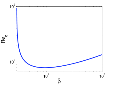
Figure 1: MRI linear stability limit for $Pm=1$

3.2 $Pm\neq 1$ behavior

The dispersion relation can no longer be solved exactly in this case, but an approximate solution can be found in the low magnetic field limit ($V_{A}\rightarrow 0$, or more precisely $V_{A}k_{z}\ll\kappa$), where marginal stability follows from a balance between the destabilizing term, and the dissipation ones. The “opposite” (high $\beta$) marginal stability limit, where destabilization is balanced by the usual Alfvénic magnetic tension, is briefly addressed at the end of this section.

In the limit of vanishing magnetic field, the dispersion relation has two relevant roots $\omega_{\eta}^{2}=0$ and $\omega_{\nu}^{2}=\kappa^{2}$. In what follows, we refer to these roots as the Alfvénic and the inertial branch, respectively. Looking for the first order correction in $V_{A}^{2}k_{z}^{2}$ to the Alfvénic branch yields the following result, which describes the MRI modes:

$$\omega=i\eta k_{z}^{2}\pm i\Bigg{(}\frac{2\Omega S}{k_{z}^{4}(\eta-\nu)^{2}+\kappa^{2}}\Bigg{)}^{1/2}V_{A}k_{z}.$$ (13)

Note that viscosity and resistivity do not play a symmetric role in this expression. Two interesting limits with respect to the magnitude of the viscosity prove useful to characterize marginal stability. As before, we maximize instability by assuming $\gamma=1$ and $k_{z}=2\pi/H$.

3.2.1 Low viscosity limit:

First consider the limit where $\nu k_{z}^{2}\ll\kappa$. In this case, Eq. (13) reduces to $\eta k^{2}=(2\Omega S/\kappa^{2})^{1/2}V_{A}k_{z}$ (where $\eta k_{z}^{2}\ll\kappa$ has been self-consistently used). Using the Lundquist number defined as $Lu=Rm\beta^{-1/2}$, this can be recast as

$$Lu=\left(\frac{2\pi}{3^{1/2}}\right)\simeq 3.6.$$ (14)

Note that our definition of the Lundquist number is not strictly identical to Turner et al. (2006) but is widely used in the MHD community In this regime, the $\omega_{\eta}^{2}\kappa^{2}$ term balances the $2\Omega SV_{A}^{2}k_{z}^{2}$ term in the dispersion relation Eq. (11). Eq. (14) corresponds to the limit found by Fleming et al. (2000). It is also related to the origin of the “dead zone” in accretion disks (see e.g Gammie 1996). This marginal stability limit is relevant to disks with low Prandtl numbers ($Pm\ll 1$) and high Reynolds numbers ($Re\gg 1$), such as YSO disks.

Also, for negligible resistivity, growth rates in this regime are given by

$$\tau^{-1}\simeq\frac{1}{2\pi}\left(\frac{2\Omega S}{\kappa^{2}}\right)V_{A}k_{z}.$$ (15)

This result is valid for $V_{A}k_{z}\lesssim\kappa$ due to our expansion scheme; it also gives the correct order of magnitude of maximum growth rates when $V_{A}k_{z}\sim\kappa$, as shown by the standard dissipationless MRI analysis.

3.2.2 High viscosity limit:

Conversely, consider the large viscosity limit, where $\nu k^{2}\gg\kappa$. The corresponding relations in this limit are

$$ReRm=\frac{3^{1/2}}{2}(2\pi)^{3}\beta^{1/2}\simeq 215\beta^{1/2}.$$ (16)

and

$$\tau^{-1}\simeq\frac{1}{2\pi}\left(\frac{2\Omega S}{\nu k_{z}^{2}}\right)V_{A}k_{z}.$$ (17)

In this regime, the $\omega_{\nu}^{2}\omega_{\eta}^{2}$ term balances the $2\Omega SV_{A}^{2}k_{z}^{2}$ term in the dispersion relation Eq. (11). The growth rates relevant here are much smaller than in the small viscosity limit, Eq. (15). In fact, Eq. (13) indicates that this is the case as soon as $\nu k_{z}^{2}\lesssim\kappa$, or equivalently, for the largest mode, when

$$Re\gtrsim 3(2\pi)^{2}/2\simeq 60.$$ (18)

This limit divides the low and high viscosity regime.

The marginal stability limit Eq.(16) obtains for large Prandtl and small Reynolds numbers. In the large Prandtl ($Pm\gg 1$) and large Reynolds number limit ($Re\gg 1$) expected in AGN disks, the growth rates of Eq. (15), or more generally of dissipationless MRI, are recovered. As before, these growth rates are expected to be valid (in order of magnitude) for $V_{A}k_{z}\lesssim\kappa$ due to our expansion scheme.

Note finally that a similar analysis can be performed for the inertial modes, but is not very informative; as they appear to be always stable.

3.2.3 High $\beta$ limit:

Although we did not investigate this case in much detail, it is apparent from Eq. (11) that when $2\Omega S=V_{A}^{2}k_{z}^{2}$ [cancellation of the last term in Eq. (11)], $\omega_{\eta}=0$ is one of the solutions to the dispersion relation. At the light of our preceding analyzes, and because this equality embodies the MRI stability limit in the ideal case, as recalled above, it is apparent that this relation is the relevant limit in a small dissipation context as well, generalizing the result found for $Pm=1$.

3.2.4 Heuristic explanation:

To explain the behavior brought to light in Eqs. (14) and (16), it is useful to recall the physical origin of the instability, as discussed, e.g., in Balbus & Hawley (2003), in the dissipation-free limit; the process is sketched on Fig. 2, for convenience. Assume for definiteness that one starts by distorting the equilibrium velocity field in the radial direction with a sinusoidal perturbation in the vertical direction: $v_{y}=v_{y_{0}}\exp\big{(}-ikz\big{)}$. The magnetic field being frozen in the fluid will also develop a radial component [first term in the right-hand side member of the linearized induction equation, Eq. (8)]; the shear will then transform this radial field in an azimuthal one [second term in the right-hand side member of the linearized induction equation, Eq. (8)]. The resulting tension force produces a momentum transfer between fluid particles that have been moved according to the imposed velocity perturbation [second term in the right-hand side member of the linearized motion equation, Eq. (8)]. This force is destabilizing if the angular velocity decreases with radius: indeed in this case, the inner particle, moving faster than the outer one, will transfer orbital momentum to the outer one, thereby reinforcing its inward motion, an effect mediated by the Coriolis force when seen in the rotating frame. In this description, marginal stability follows when the driving mechanism is balanced by the usual tension restoring force (the piece not connected to the generation of magnetic field from the mean shear).

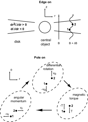
Figure 2: Sketch of the MRI mechanism (see text).

What does dissipation change to this picture ? For definiteness, let us focus on marginal stability and let us consider only resistive dissipation for the time being (“low” viscosity limit). In this limit, the magnitude of the velocity and magnetic fields in the various steps of the instability mechanism described above are controlled by dissipation processes so that one may again go through the preceding process step by step, assuming equilibrium at each step. The magnitude of the radial magnetic field in this context results from the balance between the motion driving and field dissipation:

$$-ikB_{0}v_{y}=\eta k^{2}b_{y},$$ (19)

while the shearing generation of the azimuthal field from the radial one is also balanced by resistive dissipation:

$$Sb_{y}=\eta k^{2}b_{x}.$$ (20)

Both relations follow from the induction equation in the marginal stability limit, except for the term dropped in Eq. (20), which leads to the usual magnetic tension stabilization and is of no interest in the limit considered here. The azimuthal force balance then requires that

$$(2\Omega-S)v_{y}=i\frac{kB_{0}}{\mu_{0}\rho_{0}}b_{x},$$ (21)

i.e., $\omega_{\eta}^{2}\kappa^{2}=2\Omega SV_{A}^{2}k^{2}$, once the two preceding constraints are taken into account (inclusion of $\omega$ in this line of argument does not change the result). As noted earlier, this relation directly leads to Eq. (14).

If one assumes instead that viscous dissipation exceeds the Coriolis force in magnitude, then the magnetic tension due to the generation of azimuthal field from the radial one by the shear should be balanced by viscous dissipation instead of the Coriolis force in the two horizontal components of the momentum equation, leading alternatively to $\omega_{\eta}^{2}\omega_{\nu}^{2}=2\Omega SV_{A}^{2}k^{2}$, i.e. to Eq. (16).

This also relates to the structure of MRI modes. In the limit of a very small magnetic tension restoring force, the Alfvénic branch is made of $b_{x}$ dominated modes. The other components of the magnetic field and the velocity field are of the order of $V_{A}k$ compared to $b_{x}$. Therefore, the growth rate is at first controlled by the dissipation rate of $b_{x}$, which is related to the resistivity [first term of the right hand side of Eq. 13]. The interaction of the other fields, which leads to the MRI, is controlled by a term symmetric in $\nu$ and $\eta$ [second term of Eq. 13)].

3.2.5 Generic behavior:

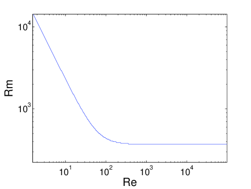
Figure 3: MRI linear stability limit in the $Pm\neq 1$ case for $\beta=10^{4}$.

A more complete view of the stability limits and growth rates implied by Eq. (11) may be obtained from exact numerical solutions for $Pm\neq 1$. Expressing this dispersion relation in terms of $\omega$ leads to the condition:

$$\omega^{4} -2ik^{2}\omega^{3}(\eta+\nu)-\omega^{2}\Big{(}a+k^{4}(\eta^{2}+\nu^{2}+4\eta\nu)+b\Big{)}$$ (22)

$$+\omega\Big{(}2ik^{6}(\eta\nu^{2}+\nu\eta^{2})+aik^{2}(\nu+\eta)+2ib\eta k^{2}\Big{)}$$

$$+\nu^{2}\eta^{2}k^{8}+a\nu\eta k^{4}+b\eta^{2}k^{4}-c=0,$$

with

$$a = 2k_{z}^{2}V_{A}^{2}$$ (23)

$$b = \kappa^{2}\gamma^{2}$$ (24)

$$c = k_{z}^{2}V_{A}^{2}(2\Omega\gamma^{2}S-k_{z}^{2}V_{A}^{2})$$ (25)

To characterize the stability limits as a function of the Reynolds and the Magnetic Reynolds number ($Rm=SH^{2}/\eta$), one needs to choose $\beta$, $\gamma$ and $k_{z}$. As in the $Pm=1$ case, we take $k_{z}=2\pi/H$ and $\gamma=1$ (which are again expected to maximize the dissipation limits), and solve the relation (22) for $\beta=10^{4}$. The resulting stability limits are shown on Fig. 3 and the corresponding growth rates on Fig. 4 (arbitrary units). These results match closely the analytical limits just discussed: a high $Re$ threshold found for $Rm\sim 371$, and a low $Re$ threshold found for ${RmRe}\sim 2.3\times 10^{4}$, both in agreement with Eqs. (14) and (16), respectively. Moreover, significantly lowered growth rates are observed when $Re\ll 60$ to $80$, as predicted by Eqs. (17) and (18). A similar behavior follows at much smaller $\beta$. For example, the observed scalings are identical, and the preceding asymptotic expressions valid within a factor of 2, down to $\beta$ values of the order of twice the critical $\beta$ limit.

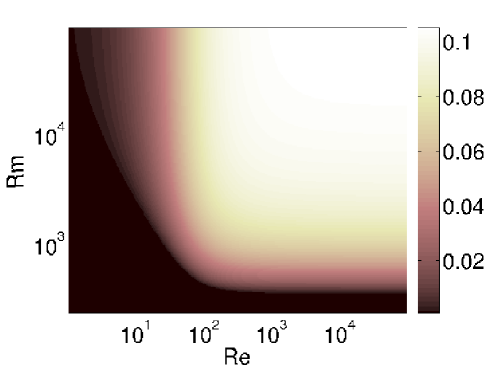
Figure 4: MRI growth rate (arbitrary unit) as a function of viscous and resistive dissipation for $\beta=10^{4}$

These results indicate that most of the stability limit behavior is captured by the approximate relations Eqs. (14) and (16) (as well as by the large field $\beta$ limit, where relevant), whose physical origin has been discussed above.

3.3 Numerics

3.3.1 Equations

Our objective is to simulate the system of Eqs. (2) and (2), with the incompressiblity condition Eq. (3), to characterize the dependence of turbulent transport on the main dimensionless numbers introduced above ($\beta$, $Re$ and $Pm$). We focus on incompressible motions; indeed, the values of $\alpha$ found in previous investigations makes us a priori expect that compressibility effects will be small. In any case, this allows us to more effectively distinguish the effects of the various physical mechanisms at work in this problem.

First, we simplify the problem from a numerical point of view by distinguishing the mean laminar shear $\bm{u}=Sy\bm{e_{x}}$ from the deviation from this mean $\bm{w}$. The resulting equations read:

$$\partial_{t}\bm{w}+\bm{w}\cdot\bm{\nabla}\bm{w} = -Sy\partial_{x}\bm{w}-\bm{\nabla}\psi+\frac{\bm{B}\times(\bm{\nabla}\times\bm{B})}{\mu_{0}\rho_{0}}$$

$$+(2\Omega-S)w_{y}\bm{e}_{x}-2\Omega w_{x}\bm{e}_{y}+\nu\Delta\bm{w}$$

$$\partial_{t}\bm{B}+\bm{w}\cdot\bm{\nabla}\bm{B} = -Sy\partial_{x}\bm{B}+\bm{B}\cdot\bm{\nabla}\bm{w}+B_{y}S\bm{e}_{x}+\eta\Delta\bm{B}$$

$$\nabla\cdot\bm{w} = 0$$

$$\nabla\cdot\bm{B} = 0$$

This system is numerically solved using a full 3D spectral code, using the classical shearing sheet boundary conditions (Hawley et al., 1995). This code is now briefly described.

3.3.2 Numerical code

The code used for these simulations is an MHD extension of the HD code used in Lesur & Longaretti (2005), and extensively described there. This code is a full 3D spectral (Fourier) code, based on FFTW libraries, parallelized using the MPI protocol. This kind of code has many advantages for the simulation of incompressible turbulence, such as:

• The incompressibility and solenoid conditions are easily implemented at machine precision, using a projector function in Fourier space.

• The energy budget is much easier to control, leading to a precise quantification of the energy losses by numerical dissipation.

• Spatial derivatives are very accurate down to the grid scale (equivalent to an infinite order finite difference scheme down to the grid scale).

The algorithm used is a classical pseudo spectral method which may be described as follows. All the derivatives are computed in Fourier space. However the nonlinear term require special treatment : in Fourier space, a real space product is a convolution, for which the computational time evolves as $n^{2}$, where $n$ is the number of grid cells. The computation time is minimized if one goes back to real space, compute the needed product and then transforms the result to Fourier space. This procedure (pseudo spectral procedure) is more efficient than a direct convolution product since the FFT computation time scales as $n\log n$. However, the finite resolution used in this procedure generates a numerical artifact commonly known as the “aliasing” effect (apparition of non physical waves near the Nyquist Frequency). This effect may be handled through a dealiazing procedure, in which the nonlinear terms are computed with a resolution 3/2 higher than the effective resolution used in the source terms (e.g., Peyret 2002).

Comparing our spectral code with a ZEUS-type finite difference code (Stone & Norman, 1992), similar results are obtained with a finite difference resolution two to three times higher than the spectral resolution. However, FFTs calculations are more computationally expensive than finite differences, leading to a final computational time equivalent for both kind of code with the same “effective” resolution.

All the simulations presented in this paper were performed with an $xyz$ resolution of $128\times 64\times 64$ with an aspect ratio of $4\times 1\times 1$, $x$ being the azimuthal direction, $y$ the radial direction and $z$ vertical direction. One may change the physical viscosity and resistivity as well as the magnetic field intensity ($\beta$). The mean magnetic field (conserved in the simulations due to the adopted boundary conditions) is aligned in the $z$ direction. White noise initial perturbations with respect to the laminar flow are introduced as initial conditions on all variables. With $\beta=100$, $Pm=1$ and $Re=3200$ one typically generates flow snapshots as shown on Fig. 5 after relaxation of transients; this flow is quite characteristic of a fully developed 3D turbulent field .

Figure 5: $w_{y}$ plot (radial velocity) for $\beta=100$, Re=3200,

3.4 MRI behavior near the instability threshold

The MRI is a weak magnetic field instability, which should be quenched for $\beta\lesssim 1$ in astrophysical disks. Since the MRI is assumed to be the source of momentum transport in disks, and as at least some disks are expected to be close to equipartition if they are to support magnetically driven ejection (Ferreira, 1997), on may wonder if this instability is efficient enough in the vicinity of the strong magnetic field stability threshold. We investigate this question in an unstratified context here (the absence of stratification significantly raises the $\beta$ stability threshold).

We present two simulations. In the first one, $\beta=100$ and $Re=3200$ (run 1); this run reproduces typical results from the literature. The second simulation is performed close the $\beta$ threshold, i.e. for $\beta=30$ and $Re=3200$. The time development of some important quantities is depicted on figs (6) and (7) for these two runs. One immediately notices a marked difference between these two simulations. On run 1, we find a classical MRI behavior, as studied by Hawley et al. (1995), characterized by $\alpha\sim 10^{-1}$ and random fluctuations of all statistical quantities. However, run 2 exhibits strong exponential growth (“bursts”) for about 100 shear times ($\sim$10 orbits), and a sudden drop of fluctuation amplitudes. This behavior is explained as follows: for such low $\beta$ only the largest wavelength mode is unstable (and not smaller scales); the mode amplitude increases for many shear times, as this mode is an exact nonlinear solution to the incompressible equations of motions (Goodman & Xu, 1994). We therefore observe the growth of the channel flow as seen by Hawley & Balbus (1992). However, as this channel solution reaches sufficiently large amplitude, secondary instabilities such as the Kelvin-Helmoltz instability quickly set in and destroy these ordered motions, and a new cycle starts (see Goodman & Xu 1994 for a detailed description of these secondary instabilities).

Note that this kind of behavior and related explanation does also apply to the low Reynolds threshold, since there the smallest scales are viscously damped and only the largest ones remain unstable. We did observe this behavior close the low Reynolds threshold, as did Fleming et al. (2000) but in an indirect way (see Figs. 2 and 4 of their paper ), and one can conclude that these bursts are characteristic of a marginally unstable MRI. Such bursts may be astrophysically relevant. Indeed, one may wonder about the MRI behavior close to the dead zone (Gammie, 1996), where presumably the magnetic Reynolds number is small, and the instability quenched. If these bursts exist in real disks, they may quickly destroy this dead zone under the effects of the strong turbulent motions observed in our simulations.

Let us have a closer look on these bursts with the help of correlation lengths defined as

$$L_{i}=\frac{\int dy_{i}\int f(x_{i})f(x_{i}-y_{i})dx_{i}}{\int f^{2}(x_{i})\,dx_{i}}$$ (26)

where $i=1,2,3$ is the direction of correlation and $f$ refers either to the velocity or magnetic field. Note that with this definition, the correlation length vanishes in the $z$ direction for a pure sinusoidal signal, and equals $1$ in the $y$ direction for a channel flow, as a consequence of the shearing sheet boundary conditions. Therefore, these correlation lengths provide us with a convenient tool to trace the presence of the channel flow solution in our simulations. We show on fig. 8 and fig. 9 the evolution of the correlation length in the $y$ and $z$ direction for the $w_{x}$ field (a similar behavior is obtained with the other field components). The behavior of correlation lengths closely follows what can be seen by monitoring the energy in the deviations from the laminar flow (fig. 7), and indicate the presence of two main regimes in this simulation. The first regime corresponds to an exponential growth (“burst”) of the channel flow, for which $L_{y}$ is found to be equal to the box size and $L_{z}=0$ (a careful examination shows that $L_{z}$ is exponentially decaying down to $10^{-10}$), indicating the presence of a purely sinusoidal mode in the $z$ direction in the burst stage. The second regime is a more classical state for 3D turbulent motion, with $L_{y}\simeq 0.5$ and $L_{z}\simeq 0.4$. Note that $L_{y}$ grows on very short time-scales, leading eventually to a new burst stage.

These correlation lengths disclose numerical artifacts in the first regime. In a real disk, one would expect a loss of correlation in the radial direction on a scale of the order of a few scale heights: indeed, the typical frequency involved in these phenomena is of the order of the Keplerian frequency and a signal can’t propagate faster than the sound speed, leading to a maximum correlation length of a few scale heights.

Similarly, the vanishingly small vertical correlation length for the channel flow solution is also an artifact of the adopted boundary conditions. A more realistic result would follow if one were to take into account the vertical stratification and set the boundary conditions far enough from the disk midplane. More generally, our results are probably not directly applicable to a real disk, but they shed some light on what the generic behavior of the MRI would look like near various stability thresholds, even though different aspect ratio and boundary conditions should be investigated before firm conclusions can be drawn.

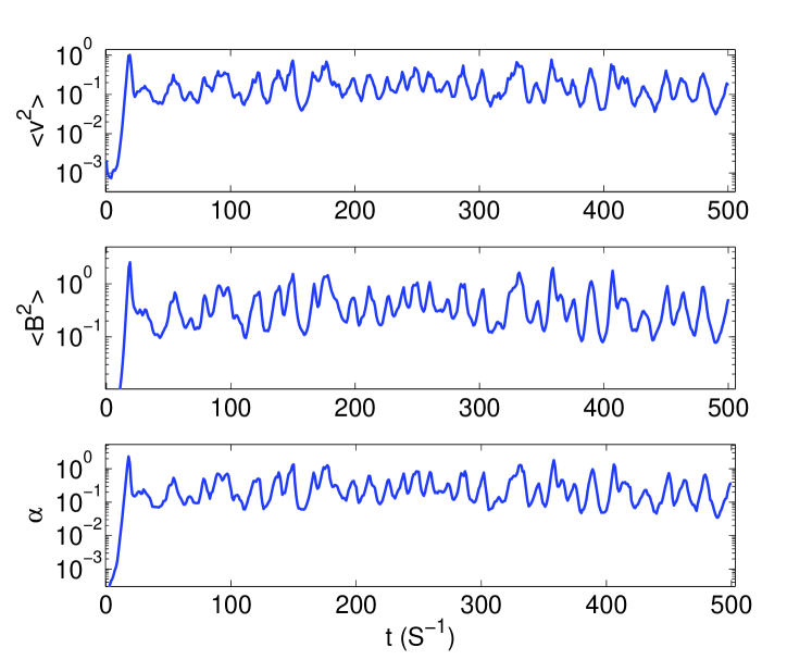
Figure 6: $\beta=100$, Re=3200 run

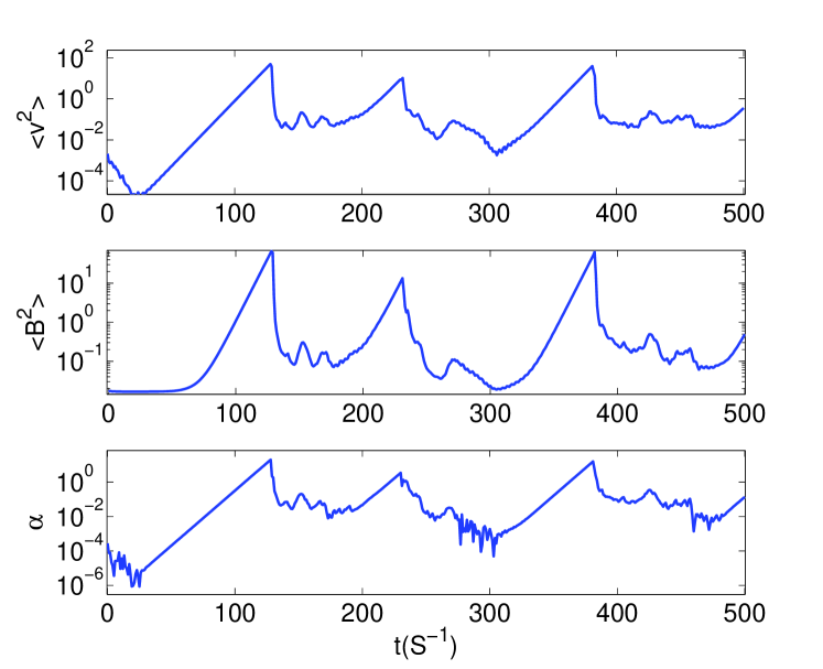
Figure 7: $\beta=30$, Re=3200 run

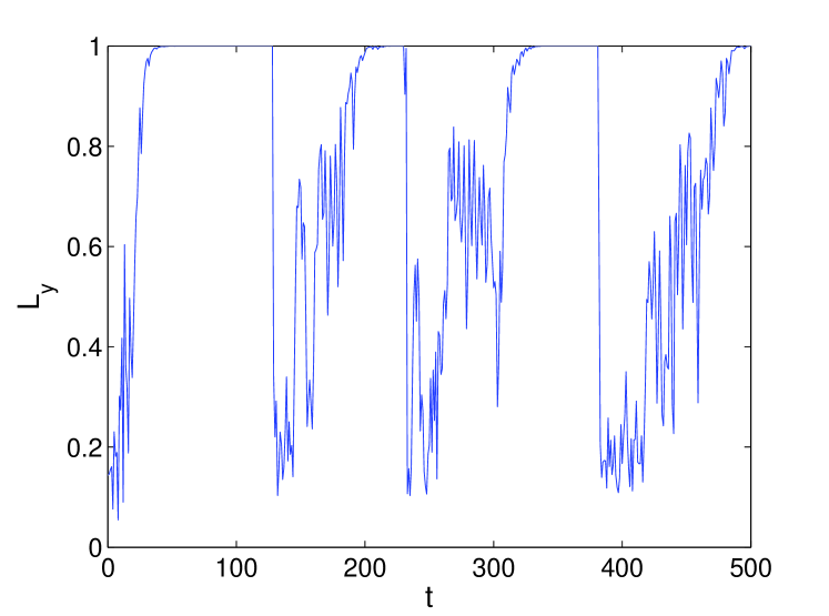
Figure 8: Correlation length of $w_{x}$ in the $y$ direction as a function of time, $\beta=30$.

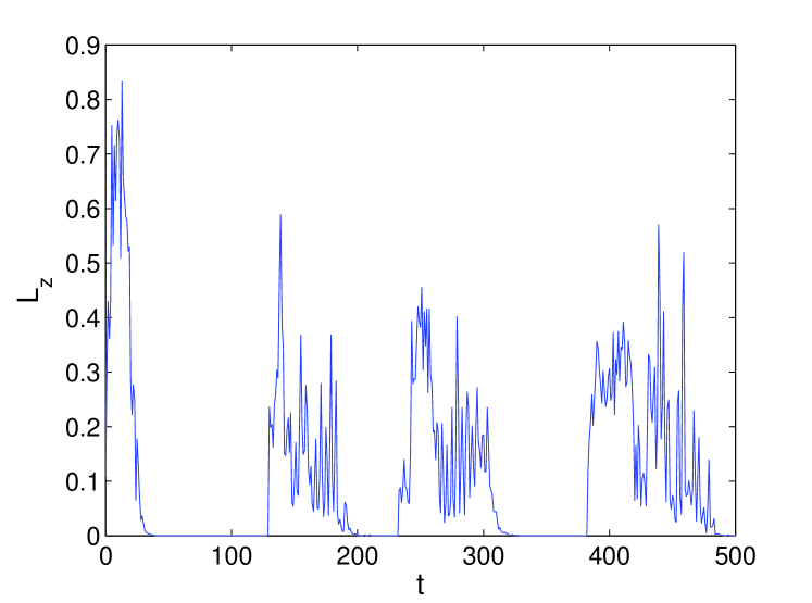
Figure 9: Correlation length of $w_{x}$ in the $z$ direction as a function of time, $\beta=30$.

Finally, the behavior exemplified in our simulations suggests that assuming $\alpha$ constant would poorly represent the transport behavior close enough to the marginal stability limit. Time-dependent transport models are needed in such a context. Real disks may not operate close to the strong field limit unless some (unknown) back-reaction loop is at work, or unless (more realistically) the magnetic field varies in a systematic way with radius throughout the disk; consequently, the bursting behavior observed here may imply a similar ejection variability in the relevant regions of jet-driving disks. Note however, that our “mean” equivalent $\alpha$ is rather large ($\alpha\simeq 5$), leading to question the role of the ignored fluid compressibility in these cases; it is quite possible that couplings to compressible modes may effectively limit the magnitude of the bursts.

3.5 Magnetic Prandtl dependence of transport coefficients

All previously published simulations were performed without numerical control of the dissipation scales and dissipation processes. However, as pointed out earlier, such a control is required to ascertain convergence. In this section, the role of the Reynolds and Prandtl numbers defined in section 3 is examined. In particular, the Prandtl number allows us to change the ratio of the viscous and resistive dissipation scales. Unfortunately, deviations from $Pm=1$ are quite demanding numerically, since one wants to resolve both the velocity and magnetic dissipations scales. We present on Fig. 10 the result of such simulations: we plot the mean transport coefficient ($\alpha$) as a function of the Prandtl number, for various Reynolds numbers (the Reynolds number quantifies the viscous dissipation scale). Statistical averages are computed over 500 shear times, and start after the first 100 shear times to avoid pollution by relaxation of the initial transient dynamics. From these plots, one finds a significant correlation between the Prandtl number and the transport coefficient, leading to

$$\alpha\propto Pm^{\delta}\qquad\mathrm{for}\left\{\begin{array}[]{c}0.12<Pm<8\\ 200<Re<6400\end{array}\right.,$$ (27)

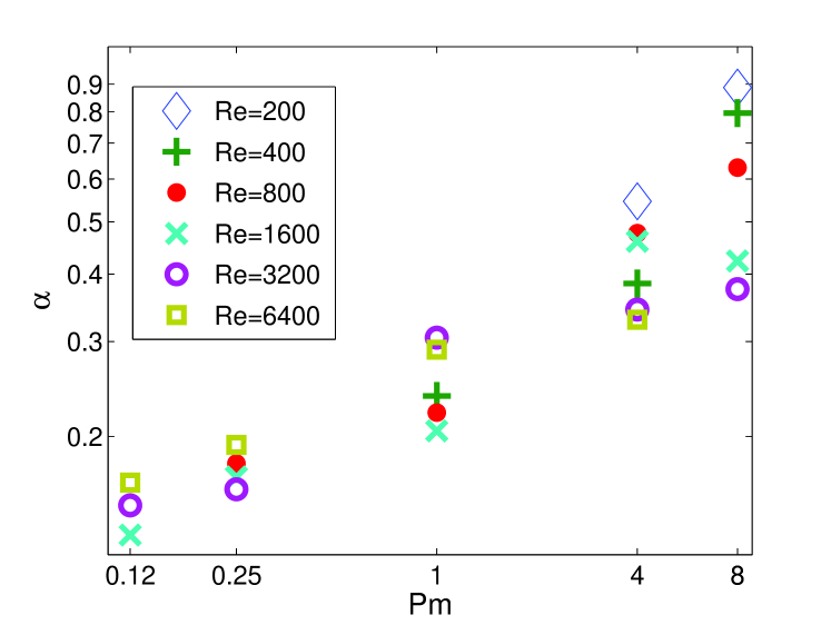
Figure 10: Prandtl effect for $\beta=100$

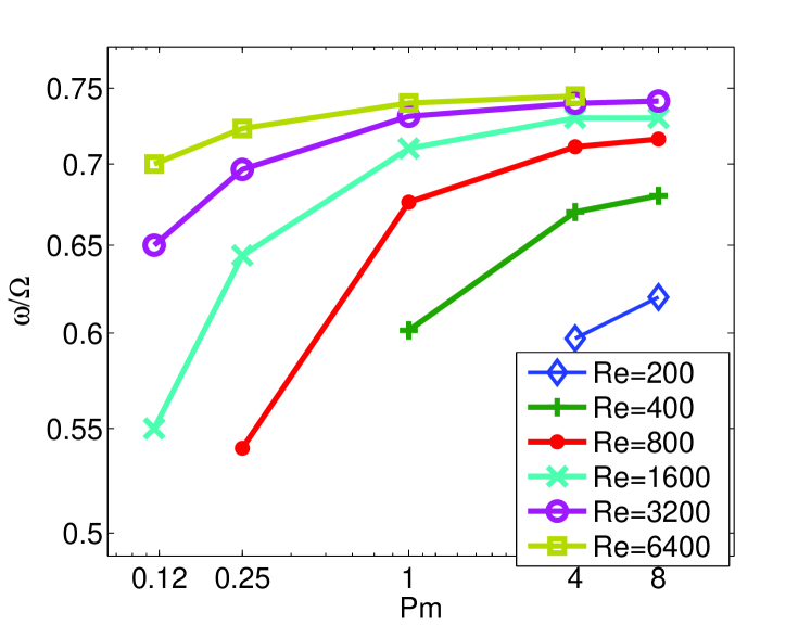
Figure 11: Linear growth rate of the largest mode for various ($Re,Pm$) at $\beta=100$

with $\delta$ in the range $0.25$ — $0.5$. Note that this results show that the transport coefficient depends on $Re$ and $Rm$ via $Pm$, at least in the $Pm$ range concidered in this paper. This may be seen on Fig. 10 as a small vertical dispersion (variation of both $Re$ and $Rm$ at constant $Pm$) compared to the effect of a single $Pm$ change. Although this section is the briefest of the paper, this result constitutes the most important finding of this investigation (and the most computationally intensive one!).

Note that the numerical results obtained at very high Reynolds number and high Prandtl number are only marginally resolved, mainly because of a very short magnetic dissipation scale. This remark may explain that the two points at $Pm=8$ lie somewhat below the mean of the other results. Our preliminary tests at higher resolution seem to show that a higher transport obtains at higher resolution at $Pm=8$ and $Re=6400$, which confirms a limit due to resolution in these high $Pm$ runs. This behavior is easily understood, since the finite numerical resolution enforces a numerical dissipation scale (roughly equal to the grid scale), which is obviously the same for the magnetic and velocity fields. Therefore, at high $Pm$, the effective magnetic dissipation scale is forced to be larger than the expected one, leading to an altered spectral distribution and a smaller “numerical Prandtl”.

One may wonder if this Prandtl dependence may be correlated to the linear growth rates discussed before. To this effect, we plot the linear growth rate of the largest mode for the different simulations used for this study on Fig. 11. Similar results follow when replacing the growth rate of the largest mode by the maximum growth rate. Although the idea of a transport efficiency controlled by the linear growth rate is widely spread in the Astrophysical community, this plot shows us that, at least for this example, the linear growth rate doesn’t explain the transport behavior observed on Fig. 10. Moreover, it appears that, as one may suspect from Eq. (13), the growth rate is not controlled only by $Pm$, but also by some complex combination of $Re$ and $Rm$. Umurhan et al. (2007) tried to get this kind of $\alpha-Pm$ correlation analytically, using a weakly non linear analysis of the channel flow. This study leads to a stronger $\alpha-Pm$ correlation with $\delta=1$ in the limit $Pm\ll 1$, which appears to be quite different from our full 3D numerical results. Note however that their analysis belongs to very different boundary conditions (rigid instead of shearing sheet) and there results are therefore not of direct relevance to our numerical investigation; nevertheless both studies point out the role of the Prandtl number. In any case, one needs to find some full nonlinear theory to explain the transport dependance on $Pm$.

The observed correlation indicates the existence of a back-reaction of the small magnetic field scales on the large ones (at least for the range of Reynolds and Prandtl numbers explored here). Note that this effect is expected to saturate at some point, since in the limit $Pm\rightarrow 0$ with $Re\rightarrow\infty$ and $Rm$ kept constant, Eq. (27) predicts a vanishing transport in spite of the existence of the linear instability. This issue is further discussed in the conclusion, the Reynolds number limitation of our investigation being the most serious here. In any case, the exact implications of these findings remain to be understood, but may potentially be quite important since the Prandtl number varies by many orders of magnitude in astrophysical objects. For example, Brandenburg & Subramanian (2005) suggest that values as small as $Pm\sim 10^{-8}$ might be found in young stellar objects, while $Pm\sim 10^{4}$ would be more typical of AGN disks. These estimates are highly uncertain; even a substantially narrower range is of course out of reach of present day computers.

Finally, this kind of back-reaction points out the potential role of small scale physics (dissipation scales) on the properties of turbulence at the largest available scales (disk height scale). This argues for a careful treatment of the role of dissipation and reconnection processes on the turbulence transport characterization.

4 Discussion

In this paper, we have investigated the role of local dimensionless numbers on the efficiency of the dimensionless turbulent transport. To this effect, we have first generalized previously published linear stability limits, to account for the presence of both viscous and resistive dissipation. Namely, we have confirmed in all cases that the large field marginal stability limit is characterized by a constant plasma $\beta$ parameter, of order 30 in the shearing sheet unstratified context (but more likely of order unity in real, stratified disks). When marginal stability follows from dissipation and not magnetic tension stabilization, we have found that the marginal stability limit is captured by two asymptotic regime: a large Reynolds ($Re$), small magnetic Reynolds one ($Rm$), with a marginal stability limit $Rm\sim\beta^{1/2}$, and a small Reynolds, large magnetic Reynolds number one, where $ReRm\sim 10^{2}\beta^{1/2}$. A phenomenological explanation has been provided for this behavior.

In the previous section, we have investigated the behavior of the MRI near the low $\beta$ instability threshold; in our simulations, $\beta=30$, a value representative of the large field threshold in our simulation box. In vertically stratified disks, this threshold obtains for much smaller values, typically $\beta\sim 1$ (Gammie & Balbus 1994). We found, somewhat unexpectedly, that turbulent transport is significantly enhanced through burst events, even surprisingly close to the marginal stability threshold. As pointed out earlier, this behavior is physical and not numerical. The use of periodic boundary conditions (vertical) or semi periodic (radial) boundary conditions may enhance the role of the channel flow solution which is responsibly for this behavior, and a real disk channel flow may break up sooner than observed in our local simulations, leading to smaller burst magnitudes. Moreover, $\alpha>1$ leads to supersonic motions and compressible numerical simulations are needed to properly quantify the phenomenon, which may exhibit new secondary compressible instabilities in such a context. All these issues lead to the conclusion that low $\beta$ MRI would produce weaker bursts and therefore smaller transport coefficient than observed in our simulation. However, there is no physical reason why the turbulence bursts would be suppressed, and we believe that these bursts may be a strong signature of regions of stratified disks where MRI-driven turbulence is driven close to the marginal stability threshold.

The most important new result reported in this paper is a correlation between the transport efficiency, and the magnetic Prandtl number, leading to a higher transport coefficient for larger Prandtl numbers. As in the case of the bursting behavior discussed above, the boundary conditions used in these simulations play some role in the result. However, the possible biases are less obvious and tests with plane radial walls need to be performed to get a grasp on boundary condition effects. Moreover, one needs to check the correlation at higher resolutions, and if possible higher Prandtl numbers, using different kind of codes to get a better characterization and a physical description of the phenomena involved in this observation.

More specifically, a puzzling fact points towards a potential bias due to the shearing sheet boundary conditions. In non-magnetized shear flows, transport in the subcritical regime, far enough from the marginal stability limit scales like $1/Rg$ where $Rg$ is the subcritical transition Reynolds number (Lesur & Longaretti, 2005). Closer to the marginal stability limit, and in the supercritical regime (e.g., when the Rayleigh stability criterion is not satisfied), transport is enhanced with respect to this scaling, but one always has $\alpha<1/Rc$ where $Rc$ is the critical Reynolds number of linear instability. However, for MRI-driven turbulence, one has $\alpha>$ or$\gg 1/Rc$, as can be checked from our results. Close to the marginal stability limit, this enhanced efficiency is related to the existence of the channel flow solution, as discussed above. As each linear mode is a nonlinear solution to the incompressible problem, one may ask whether this enhanced transport, which is observed also far from the marginal stability limit, is not an artifact of the shearing sheet boundary condition, which allows such nonlinear coherent modes to develop. This behavior is not necessarily unphysical or irrelevant to actual disk systems, but this point needs to be checked in the future.

Finally, let us come back to the magnetic Prandtl number dependence of $\alpha$. As pointed out earlier, the dependence of the transport efficiency on the magnetic Prandtl number indicates a back-reaction of small scales on large ones. We make here a few comments on this feature. In particular, we shall argue that this behavior must saturate at low and large enough $Pm$. The magnetic Prandtl number is related to the ratio of the viscous $l_{\nu}$ and resistive $l_{\eta}$ dissipation scales, the exact relation depending on the shape of the turbulent energy spectrum. Generally speaking, the Prandtl number varies monotonically with the ratio $l_{\nu}/l_{\eta}$, and one expects $Pm\ll 1$ (resp. $Pm\gg 1$) when $l_{\nu}/l_{\eta}\ll 1$ (resp. $l_{\nu}/l_{\eta}\gg 1$). The spectrum of the largest scales tends to be flatter than usual turbulent spectra due to the role of the linear instability, down to the scale where the magnetic tension prevents the instability to occur (most probably, this “instability sector” of the spectrum only represents a small part of the overall turbulent spectra of actual disks, because of their enormous Reynolds numbers). Leaving aside these largest scales, for $Pm\ll 1$, the spectrum is expected to be Kolmogorovian and anisotropic down to the resistive dissipation scale (Goldreich & Sridhar, 1995), while below this scale and down to the viscous scale, the velocity spectrum is the usual Kolmogorov velocity spectrum and the magnetic spectrum drops much faster. On the other hand, for $Pm\gg 1$, the spectrum should be Kolmogorovian down to the viscous dissipation scale (Goldreich & Sridhar, 1995), while the magnetic spectrum should scale like $k^{-1}$ below the viscous dissipation scale and down to resistive scale (Cho et al., 2003). It is therefore tempting to see in a difference of accumulation of magnetic energy at small scales the cause of the back-reaction of these scales to the largest ones, which would create the observed magnetic Prandtl number dependence of the turbulent transport efficiency. Nevertheless, in both small and large Prandtl number settings, turbulent motions in the inertial range are random in phase, so that one expects that to lowest order, coupling of the turbulent spectrum with the largest MRI unstable scales vanishes. To next order, the steepness of the Kolmogorov spectrum indicates that the strength of the coupling decreases with increasing Reynolds number in the vicinity of the viscous dissipation scale, suggesting that at large enough Reynolds numbers, the Prandtl dependence should saturate (a potential caveat to this argument being the possible role played by a small scale field generation through dynamo action). Such a saturation was not observed in our simulations, although a weak dependence of our results on the magnitude of the Reynolds number may be detected on Fig. 10; however, such an effect might also arise from resolution requirements, which makes our lower Reynolds number results confined to the larger Prandtl number range. Unfortunately, our results can hardly be improved upon with the present generation of computers, leaving the question of the Reynolds number saturation of the Prandtl number dependence open, as well as the overall difference in transport efficiency between the small and large Prandtl number cases. Resolving this issue is crucial to ascertain the role of the magneto-rotational instability in disk transport.

References

- Arlt & Urpin (2004) Arlt R., Urpin V., 2004, A&A, 426, 755
- Balbus (2003) Balbus S. A., 2003, ARA&A, 41, 555
- Balbus & Hawley (1991) Balbus S. A., Hawley J. F., 1991, ApJ, 376, 214
- Balbus & Hawley (2003) Balbus S. A., Hawley J. F., 2003, in Falgarone E., Passot T., eds, LNP Vol. 614: Turbulence and Magnetic Fields in Astrophysics Numerical Simulations of MHD Turbulence in Accretion Disks. pp 329–348
- Balbus et al. (1996) Balbus S. A., Hawley J. F., Stone J. M., 1996, ApJ, 467, 76
- Balbus & Terquem (2001) Balbus S. A., Terquem C., 2001, Astrophys. J., 552, 235
- Blaes & Balbus (1994) Blaes O. M., Balbus S. A., 1994, Astrophys. J., 421, 163
- Brandenburg et al. (1995) Brandenburg A., Nordlund A., Stein R. F., Torkelsson U., 1995, ApJ, 446, 741
- Brandenburg & Subramanian (2005) Brandenburg A., Subramanian K., 2005, Phys. Rep., 417, 1
- Cho et al. (2003) Cho J., Lazarian A., Vishniac E. T., 2003, ApJ, 595, 812
- Dubrulle et al. (2005) Dubrulle B., Marié L., Normand C., Richard D., Hersant F., Zahn J.-P., 2005, A&A, 429, 1
- Ferreira (1997) Ferreira J., 1997, A&A, 319, 340
- Fleming et al. (2000) Fleming T. P., Stone J. M., Hawley J. F., 2000, ApJ, 530, 464
- Gammie (1996) Gammie C. F., 1996, ApJ, 457, 355
- Gammie & Balbus (1994) Gammie C. F., Balbus S. A., 1994, MNRAS, 270, 138
- Gardiner & Stone (2005) Gardiner T. A., Stone J. M., 2005, in de Gouveia dal Pino E. M., Lugones G., Lazarian A., eds, AIP Conf. Proc. 784: Magnetic Fields in the Universe: From Laboratory and Stars to Primordial Structures. Energetics in MRI driven Turbulence. pp 475–488
- Goldreich & Sridhar (1995) Goldreich P., Sridhar S., 1995, ApJ, 438, 763
- Goodman & Xu (1994) Goodman J., Xu G., 1994, ApJ, 432, 213
- Hawley (2000) Hawley J. F., 2000, ApJ, 528, 462
- Hawley & Balbus (1992) Hawley J. F., Balbus S. A., 1992, ApJ, 400, 595
- Hawley et al. (1999) Hawley J. F., Balbus S. A., Winters W. F., 1999, ApJ, 518, 394
- Hawley et al. (1995) Hawley J. F., Gammie C. F., Balbus S. A., 1995, ApJ, 440, 742
- Ji et al. (2006) Ji H., Burin M., Schartman E., Goodman J., 2006, Nature, 444, 343
- Ji et al. (2001) Ji H., Goodman J., Kageyama A., 2001, MNRAS, 325, L1
- Johnson & Gammie (2006) Johnson B. M., Gammie C. F., 2006, ApJ, 636, 63
- Klahr & Bodenheimer (2003) Klahr H. H., Bodenheimer P., 2003, ApJ, 582, 869
- Lesur & Longaretti (2005) Lesur G., Longaretti P.-Y., 2005, A&A, 444, 25
- Longaretti & Lesur (2007) Longaretti P.-Y., Lesur G., 2007, In preparation for A&A
- Peyret (2002) Peyret R., 2002, Spectral Methods for Incompressible Viscous Flow. Springer
- Richard (2001) Richard D., 2001, PhD thesis, Université de Paris VII
- Richard et al. (2001) Richard D., Dauchot O., Zahn J.-P., 2001, in Proc. of the 12th Couette-Taylor Workshop, Evanston, USA Subcritical Instabilities of Astrophysical Interest in Couette-Taylor System
- Richard & Zahn (1999) Richard D., Zahn J., 1999, A&A, 347, 734
- Rüdiger & Shalybkov (2002) Rüdiger G., Shalybkov D., 2002, Phys. Rev. E, 66, 016307
- Shakura & Sunyaev (1973) Shakura N. I., Sunyaev R. A., 1973, A&A, 24, 337
- Shalybkov & Ruediger (2005) Shalybkov D., Ruediger G., 2005, A&A, 438, 411
- Stone et al. (1996) Stone J. M., Hawley J. F., Gammie C. F., Balbus S. A., 1996, ApJ, 463, 656
- Stone & Norman (1992) Stone J. M., Norman M. L., 1992, ApJs, 80, 753
- Turner et al. (2006) Turner N. J., Sano T., Dziourkevitch N., 2006, astro-ph/0612552
- Umurhan et al. (2007) Umurhan O. M., Menou K., Regev O., 2007, Phys. Rev. Let., 98, 034501
- Urpin (2003) Urpin V., 2003, A&A, 404, 397
- Wardle (1999) Wardle M., 1999, MNRAS, 307, 849