Dynamical stability for finite quantum spin chains against a time-periodic inhomogeneous perturbation

Abstract

We investigate dynamical stability of the ground state against a time-periodic and spatially-inhomogeneous magnetic field for finite quantum XXZ spin chains. We use the survival probability as a measure of stability and demonstrate that it decays as $P(t)\propto t^{-1/2}$ under a certain condition. The dynamical properties should also be related to the level statistics of the XXZ spin chains with a constant spatially-inhomogeneous magnetic field. The level statistics depends on the anisotropy parameter and the field strength. We show how the survival probability depends on the anisotropy parameter, the strength and frequency of the field.

1 Introduction

Dynamical stability of quantum systems was studied from various viewpoints, e.g. from those of quantum chaos and energy diffusion in general [1, 2, 3]. In the field of quantum information, a lot of attention has been paid to the fidelity, which also describes dynamical stability [4, 5, 6, 7, 8]. The fidelity is defined as $F(t)=|\langle\psi(t)|\psi_{\delta}(t)\rangle|^{2}$, where $|\psi(t)\rangle=U_{0}(t)|\psi\rangle$ and $|\psi_{\delta}(t)\rangle=U_{\delta}(t)|\psi\rangle$ are unperturbed ($\delta=0$) and perturbed ($\delta\neq 0$) time evolutions, respectively. When the initial state $|\psi\rangle$ is an eigenstate of the unperturbed Hamiltonian, $F(t)$ coincides with a survival probability. The fidelity and the survival probability are also studied in the context of quantum irreversibility [9, 10, 11]. Those studies on fidelity, survival probability and energy diffusion have so far concentrated on highly-excited states or coherent states in random matrix models and kicked spin models. In real physics of condensed matter, however, it is more essential to elucidate the dynamical stability of the ground state for many-body quantum systems, which are non-integrable, against perturbations.

The properties of dynamical stability can depend on the level statistics of systems. Recently, the level statistics of XXZ spin chains with a time-independent random magnetic field is studied in Ref. [12]. When the anisotropy parameter $\Delta$ is nonzero, Gaussian orthogonal ensemble (GOE) level statistics appears for a large field although Poisson-like level statistics is seen for a small field. When $\Delta=0$, however, the level statistics always shows Poissonian behavior. Therefore, it is desirable to know how a time-periodic random field will affect the dynamics of quantum spin systems with and without GOE level statistics.

In this paper, we will study the dynamical stability of quantum XXZ spin chains against perturbations induced by a time-periodic and spatially-inhomogeneous magnetic field. We use the survival probability as a measure of the dynamical stability and show how the survival probability is related to the level statistics. By theoretical and numerical analysis, we will demonstrate that normal diffusion occurs in the linear response region. Numerical analysis will also exhibit how the survival probability depends on the anisotropy parameter $\Delta$, the field strength and the field frequency. This work will complement the latest study on the energy diffusion in a frustrated spin system with a non-random magnetic field [13].

The organization of the paper is as follows: In Sec. 2, we introduce the model and briefly describe our numerical method. In Sec. 3, the survival probability $P(t)$ is investigated in an analytical way. It is suggested that $P(t)$ should show a power-law decay on some assumptions. Numerical results will be shown in Sec. 4. The parameter dependence of $P(t)$ is discussed. Conclusions are given in Sec. 5

2 Model and method

The Hamiltonian of the quantum XXZ spin chain on $L$ sites under the time-periodic and spatially-inhomogeneous magnetic field is given by

$$\mathcal{H}(t)=\mathcal{H}_{0}+\mathcal{H}_{1}(t),$$ (1)

where

$$\mathcal{H}_{0}=J\sum_{j=1}^{L}(S^{x}_{j}S^{x}_{j+1}+S^{y}_{j}S^{y}_{j+1}+\Delta S^{z}_{j}S^{z}_{j+1}),$$ (2)

$$\mathcal{H}_{1}(t)=\sum_{j=1}^{L}B_{j}\sin(\omega t)S^{z}_{j}.$$ (3)

Here, $S^{\alpha}_{j}=(1/2)\sigma^{\alpha}_{j}$ and ($\sigma^{x}_{j}$, $\sigma^{y}_{j}$, $\sigma^{z}_{j}$) is the $j$th-site Pauli matrix; the periodic boundary conditions are imposed. The parameters $J$ and $\Delta$ are nearest-neighbor exchange interactions and the anisotropy parameter, respectively. The local field strength $B_{j}$’s are uncorrelated random numbers that obey a Gaussian distribution with the following average and variance:

$$\langle B_{j}\rangle=0,$$ (4)

$$\langle B_{j}B_{k}\rangle=B_{0}^{2}\delta_{jk}.$$ (5)

Before calculating the time evolution, we note the symmetries of the model. In the absence of the perturbation [$\mathcal{H}_{1}(t)=0$], eigenstates are classified by $z$ component of total spin $S^{z}_{\rm tot}$ ($=\sum_{j=1}^{L}S^{z}_{j}$), total wave number ($K$), parity (in the special cases of $K=0,\pi$) and spin reversal (for $S^{z}_{\rm tot}=0$). Eigenstates with different symmetries are uncorrelated. When $\mathcal{H}_{1}(t)\neq 0$, only $S^{z}_{\rm tot}$ is conserved, and manifolds with different wave numbers, parity or spin reversal become mixed. Here we choose the $S^{z}_{\rm tot}=0$ manifold. It should be noted that no transition can occur if the magnetic field is homogeneous.

Let us define the survival probability as

$$P(t)=\left\langle|\langle\psi(0)|\psi(t)\rangle|^{2}\right\rangle_{\rm ave}=\left\langle\tilde{P}(t)\right\rangle_{\rm ave},$$ (6)

where $\langle\rangle_{\rm ave}$ means the average over the random magnetic field. We numerically calculate $\tilde{P}(t)$ for 100 samples of spin dynamics that starts from the identical initial state but is perturbed by different sets of $B_{j}$’s. The average of $\tilde{P}(t)$’s over those samples gives $P(s)$. We choose the ground state of $\mathcal{H}_{0}$ as the initial state $|\psi(0)\rangle$. $|\psi(t)\rangle$ is a solution of the time-dependent Schrödinger equation

$$i\hbar\frac{\partial}{\partial t}|\psi(t)\rangle=\mathcal{H}(t)|\psi(t)\rangle=[\mathcal{H}_{0}+\mathcal{H}_{1}(t)]|\psi(t)\rangle.$$ (7)

In our numerical calculation, we take $\hbar=1$ for convenience. The solution consists of a sequence of the infinitesimal processes as

$$|\psi(t)\rangle=U(t;t-\Delta t)U(t-\Delta t;t-2\Delta t)\ldots U(\Delta t;0)|\psi(0)\rangle.$$ (8)

To calculate a time evolution operator $U(t+\Delta t;t)$ for each time step $\Delta t$ ($=10^{-3}$), we use the fourth-order decomposition formula for the exponential operator [13, 14]. Our numerical calculation below is mainly carried out on the system of $L=12$, whose $S^{z}_{\rm tot}=0$ manifold involves 924 levels. Here we note that there is a rather large energy gap between the ground state and the first excited state because of the finite system size, while there is no gap in the unperturbed system for $|\Delta|<1$ in the thermodynamic limit.

3 Theoretical analysis

Now we analytically investigate the short-time behavior of the survival probability. While applying the method cultivated in the context of energy diffusion [1], we will choose the ground state as an initial state and take the average over the random magnetic field. Let us expand the wave function $|\psi(t)\rangle$ in an adiabatic basis:

$$|\psi(t)\rangle=\sum_{j}a_{j}(t)e^{-i\theta_{j}(t)}|\psi(t)\rangle.$$ (9)

Here,

$$\theta_{j}(t)=\frac{1}{\hbar}\int_{0}^{t}{\rm d}t^{\prime}E_{j}(t^{\prime}),$$ (10)

and $E_{j}(t)$ is the eigenvalue of the $j$th state at time $t$:

$$\mathcal{H}(t)|j(t)\rangle=E_{j}(t)|j(t)\rangle.$$ (11)

Let us notice that $\mathcal{H}(t)=\mathcal{H}_{0}$ at $t=nT$, where $n$ is an integer and $T=2\pi/\omega$. The eigenvalues and eigenstates of the unperturbed Hamiltonian are supposed to be well solved:

$$\mathcal{H}_{0}|\phi_{j}\rangle=\varepsilon_{j}|\phi_{j}\rangle.$$ (12)

Substituting Eq. (9) into Eq. (7) and multiplying $\langle k(t)|$ on the left, we obtain

$$\dot{a}_{k}(t)=-\sum_{j(\neq k)}\frac{\big{\langle}k(t)\big{|}\frac{{\rm d}\mathcal{H}(t)}{{\rm d}t}\big{|}j(t)\big{\rangle}}{E_{k}(t)-E_{j}(t)}e^{i[\theta_{k}(t)-\theta_{j}(t)]}a_{j}(t).$$ (13)

Here we notice that the phases of the eigenstates are chosen so as to satisfy $\langle j(t)|\frac{\rm d}{{\rm d}t}|j(t)\rangle=0$. As $\mathcal{H}_{1}(t)=Z\sin\omega t$,

$$\dot{a}_{k}(t)=\omega\cos\omega t\sum_{j(\neq k)}\frac{\langle k(t)|Z|j(t)\rangle}{E_{k}(t)-E_{j}(t)}e^{i[\theta_{k}(t)-\theta_{j}(t)]}a_{j}(t).$$ (14)

Integrating Eq. (14), we have

$$a_{k}(t)=a_{k}(0)+\omega\int_{0}^{t}{\rm d}s\cos\omega s\sum_{j(\neq k)}\tilde{Z}_{kj}(s)e^{i[\theta_{k}(s)-\theta_{j}(s)]}a_{j}(s),$$ (15)

where $\tilde{Z}_{kj}(t)\equiv\langle k(t)|Z|j(t)\rangle/[E_{k}(t)-E_{j}(t)]$. Before deriving the survival probability, we need to calculate $|a_{k}(t)|^{2}$.

$$|a_{k}(t)|^{2} = |a_{k}(0)|^{2}+2{\rm Re}\left[\omega\int_{0}^{t}{\rm d}s_{1}\cos\omega s_{1}\sum_{j(\neq k)}\tilde{Z}_{kj}(s_{1})e^{i[\theta_{k}(s_{1})-\theta_{j}(s_{1})]}a_{j}(s_{1})a_{k}^{*}(0)\right]$$ (16)

$$+ \omega^{2}\int_{0}^{t}{\rm d}s_{1}\int_{0}^{t}{\rm d}s_{2}\cos\omega s_{1}\cos\omega s_{2}\sum_{j(\neq k)}\sum_{j^{\prime}(\neq k)}\tilde{Z}_{kj}(s_{1})\tilde{Z}_{kj^{\prime}}^{*}(s_{2})$$

$$\times e^{i[\theta_{k}(s_{1})-\theta_{j}(s_{1})-\theta_{k}(s_{2})+\theta_{j^{\prime}}(s_{2})]}a_{j}(s_{1})a_{j^{\prime}}^{*}(s_{2}).$$

Using Eq. (15) in the second term of the right hand side of Eq. (16), we obtain

$$|a_{k}(t)|^{2} = |a_{k}(0)|^{2}+2{\rm Re}\left[\omega\int_{0}^{t}{\rm d}s_{1}\cos\omega s_{1}\sum_{j(\neq k)}\tilde{Z}_{kj}(s_{1})e^{i[\theta_{k}(s_{1})-\theta_{j}(s_{1})]}|a_{k}(0)|^{2}\right]$$ (17)

$$+2{\rm Re}\left[\omega^{2}\int_{0}^{t}{\rm d}s_{1}\int_{0}^{s_{1}}{\rm d}s_{2}\cos\omega s_{1}\cos\omega s_{2}\sum_{j(\neq k)}\sum_{j^{\prime}(\neq j)}\tilde{Z}_{kj}(s_{1})\tilde{Z}_{jj^{\prime}}(s_{2})\right.$$

$$\quad\quad\times e^{i[\theta_{k}(s_{1})-\theta_{j}(s_{1})+\theta_{j}(s_{2})-\theta_{j^{\prime}}(s_{2})]}a_{j^{\prime}}(s_{2})a_{k}^{*}(0)\Biggr{]}$$

$$+\omega^{2}\int_{0}^{t}{\rm d}s_{1}\int_{0}^{t}{\rm d}s_{2}\cos\omega s_{1}\cos\omega s_{2}\sum_{j(\neq k)}\sum_{j^{\prime}(\neq k)}\tilde{Z}_{kj}(s_{1})\tilde{Z}_{kj^{\prime}}^{*}(s_{2})$$

$$\quad\quad\times e^{i[\theta_{k}(s_{1})-\theta_{j}(s_{1})-\theta_{k}(s_{2})+\theta_{j^{\prime}}(s_{2})]}a_{j}(s_{1})a_{j^{\prime}}^{*}(s_{2}).$$

Now let us define an occupation probability distribution:

$$P_{k}(t)\equiv\left\langle|\langle\phi_{k}|\psi(t)\rangle|^{2}\right\rangle_{\rm ave}=\left\langle\left|\langle\phi_{k}|\sum_{j}a_{j}(t)e^{-i\theta_{j}(t)}|j(t)\rangle\right|^{2}\right\rangle_{\rm ave}.$$ (18)

In particular, $P_{k}(t_{n})=\left\langle|a_{k}(t_{n})|^{2}\right\rangle_{\rm ave}$ when $t=t_{n}\equiv nT$. The survival probability $P(t)$ is defined by $P_{I}(t)$ when the initial state is $|\phi_{I}\rangle$. In other words, the initial condition is $P_{k}(0)=\delta_{kI}$. From Eq. (4), we can say

$$\langle\tilde{Z}_{kj}(t)\rangle_{\rm ave}=0.$$ (19)

Considering Eq. (5), we assume that

$$\langle\tilde{Z}_{kj}(t)\tilde{Z}^{*}_{k^{\prime}j^{\prime}}(t^{\prime})\rangle_{\rm ave}=B_{0}^{2}\delta_{kk^{\prime}}\delta_{jj^{\prime}}f(k,j)g(t)\delta(t-t^{\prime}).$$ (20)

Here, $f(k,j)\sim p_{k,j}(\varepsilon_{k}-\varepsilon_{j})^{-2}$, and $p_{k,j}$ is supposed to correspond to the transition probability between $|\phi_{k}\rangle$ and $|\phi_{j}\rangle$. The factor $(\varepsilon_{k}-\varepsilon_{j})^{-2}$ comes from the denominator of $\tilde{Z}_{kj}(t)$. We considered that the time average of $E_{j}(t)$ is about $\varepsilon_{j}$. And $g(t)$ is a periodic function whose frequency $2\omega$ since $\tilde{Z}_{kj}(t)$ should be a function with a frequency $\omega$. Using Eqs. (19) and (20), $P_{k}(t_{n})$ is approximately given by the following for $k=I$:

$$P_{k}(t_{n})\simeq 1+\omega^{2}B_{0}^{2}\int_{0}^{t_{n}}{\rm d}s\cos^{2}\omega s\sum_{j(\neq k)}f(k,j)g(s)\left\{\langle|a_{j}(s)|^{2}\rangle_{\rm ave}-\langle|a_{k}(s)|^{2}\rangle_{\rm ave}\right\}.$$ (21)

Here we assume that the integrands of Eq. (21) have almost constant values from $t_{n}$ to $t_{n+1}$. Then we obtain

$$P_{k}(t_{n+1})-P_{k}(t_{n})=\omega^{2}B_{0}^{2}\gamma T\sum_{j(\neq k)}\frac{p_{k,j}}{(\varepsilon_{j}-\varepsilon_{k})^{2}}[P_{j}(t_{n})-P_{k}(t_{n})],$$ (22)

where $\gamma$ is a constant. Let us consider a continuous distribution $P(x,t)$. Then we may apply the following correspondences: $P_{k}(t_{n})\to P(x,t)$ and $\varepsilon_{j}-\varepsilon_{k}\to\Delta x$. If $p_{k+1,k}/(\varepsilon_{k+1}-\varepsilon_{k})^{2}$ is large enough, compared with $p_{k+2,k}/(\varepsilon_{k+2}-\varepsilon_{k})^{2}$, Eq. (22) can be approximated by a diffusion equation

$$\frac{\partial P(x,t)}{\partial t}=D\frac{\partial^{2}P(x,t)}{\partial x^{2}},$$ (23)

where $D=\omega^{2}B_{0}^{2}\gamma$. The solution of the diffusion equation is generally given by $P(x,t)=(4\pi Dt)^{-1/2}\exp(-x^{2}/4Dt)$. Therefore, if the assumptions described above is valid, the survival probability $P(t)$ [$=P(0,t)$] should show a power low decay $\sim t^{-1/2}$ for $t=t_{n}=nT$.

However, such a normal diffusion is expected to occur only for the linear response regime, where the perturbation is not very large and the perturbation theory is valid. If the perturbation is very strong, Eq. (23) cannot be derived from Eq. (22) because $p_{k+i,k}/(\varepsilon_{k+i}-\varepsilon_{k})^{2}$ for $i\geq 2$ is not negligible under large perturbation. In the non-perturbative regime, where the perturbation is so strong that the perturbation theory fails, $P(t)$ is expected to decay faster than in the linear response regime.

The spectral properties of the Hamiltonian should also be related to the survival probability. When the level statistics shows GOE, the smooth level density due to a lot of level repulsion guarantees the continuum approximation used for obtaining Eq. (23). In the case of Poissonian level statistics, however, levels tend to make clusters and $p_{k+i,k}/(\varepsilon_{k+i}-\varepsilon_{k})^{2}$ for $i\geq 2$ is not always negligible. Therefore, Eq. (23) is not appropriate for that case. It is expected that the survival probability here shows a different behavior from that of a GOE case.

4 Numerical results

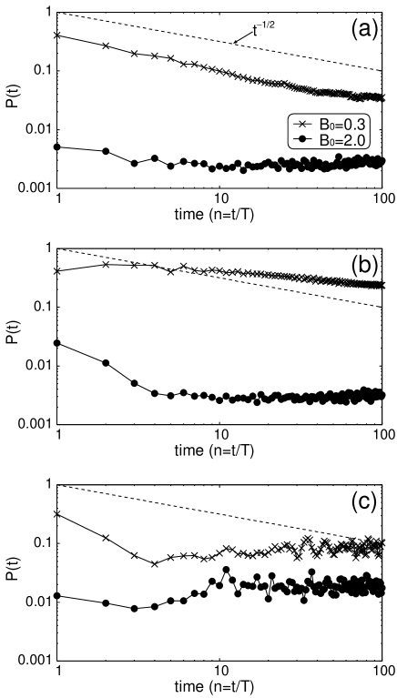
Figure 1: Survival probability $P(t)$ for (a) $\Delta=1$, $\omega=1.0$, (b) $\Delta=1$, $\omega=0.5$, (c) $\Delta=0$, $\omega=1.0$. The crosses ($\times$) are for $B_{0}=0.3$ and the solid circles ($\bullet$) are for $B_{0}=2.0$. The dashed line is just an eye guide for $P(t)\propto t^{-1/2}$.

Figure 1 shows log-log plots of $P(t)$ at each period of time. In Fig. 1(a), where $\Delta=1$ and $\omega=1.0$, $P(t)$ for $B_{0}=0.3$ decays as $P(t)\propto t^{-1/2}$. The behavior is consistent with the theoretical result in the previous section. For $B_{0}=2.0$, however, $P(t)$ decays very fast and goes down to a saturation value in a short time. The saturation value is estimated to be about 0.002 if the occupation probability spreads homogeneously over all levels. When $t=nT$, the number of levels is $489$ but not $924$, which is the number of the Hilbert space of the system, since there are many degeneracies. In Fig. 1(b), where $\Delta=1$ and $\omega=0.5$, $P(t)$ for $B_{0}=0.3$ shows slower decay than $P(t)\propto t^{-1/2}$. This case ($\omega=0.5$ and $B_{0}=0.3$) may corresponds to the near-adiabatic case. Namely, energy diffusion is slow since the perturbation is small and slow. On the other hand, $P(t)$ for $B_{0}=2.0$ decays faster than $P(t)\propto t^{-1/2}$ at first and goes down to the saturation value. Those properties of $P(t)$ seen in Figs. 1(a) and 1(b) are consistent with the expectation mentioned in the previous section. Namely, the survival probability behaves as $P(t)\propto t^{-1/2}$ in the linear response regime, and $P(t)$ decays faster than $t^{-1/2}$ in the non-perturbative regime.

The behavior of $P(t)$ in Fig. 1(c), where $\Delta=0$ and $\omega=1.0$, is very different from that of Figs. 1(a) and 1(b). For both $B_{0}=0.3$ and $B_{0}=2.0$, $P(t)$ rapidly decays and seems to saturate to a higher value than the saturation value in Figs. 1(a) and 1(b). For $\Delta=0$, the value is estimated to be about 0.02 if the occupation probability spreads homogeneously over the all levels. We may say that an anomalous diffusion occurs for $\Delta=0$. The anomalous diffusion is responsible for the properties of energy levels. Namely, when $\Delta=0$, the level statistics is Poissonian, although GOE level statistics is observed for $\Delta=1$ [12]. When the level statistics is Poissonian, which implies the appearance of level clustering, it is expected that the occupation probability distribution does not broaden very much but forms a wave packet in energy space and moves to higher levels. The wave packet reflects like a soliton at the highest levels and moves back to lower levels and reflects again at the lowest energy levels since the system size is finite. Such behavior was suggested in energy diffusion for a near-integrable system in Ref. [13]. Since we take the average over the random field such soliton-like behavior is also averaged. The behavior of the soliton-like wave packet is different in each trial. Therefore, the averaged survival probability has very rough data for $\Delta=0$.

5 Conclusions

We have investigated the survival probability $P(t)$ of XXZ spin chains under spatially-random and time-periodic field. The survival probability decays as $P(t)\propto t^{-1/2}$ in the linear response regime. The property was derived theoretically and confirmed by numerical calculation. Numerical results also demonstrated that $P(t)$ decays more slowly for small $B_{0}$ or $\omega$ than $t^{-1/2}$ and faster for large $B_{0}$ or $\omega$. When $\Delta=0$, however, $P(t)$ decays and soon goes down to a saturation value. The difference between the behavior for $\Delta=1$ and for $\Delta=0$ is caused by the property of energy levels, i.e. level-clustering or level-repulsion, for each $\Delta$.

Acknowledgement

We would like to thank M. Wilkinson for fruitful discussion and T. S. Monteiro for suggestion. The present study was partially supported by the Grant-in-Aid for JSPS Research Fellowships for Young Scientists.

References

- [1] Wilkinson M and Austin EJ. A random matrix model for the non-perturbative response of a complex quantum system. J Phys A, 1995;28:2277-2296.
- [2] Cohen D. Driven Chaotic Mesoscopic Systems, Dissipation and Decoherence. Lect Notes Phys, 2002;597:317-350.
- [3] Cohen D and Kottos T. Non-perturbative response: chaos versus disorder. J Phys A, 2003;36:10151-10158
- [4] Benenti G, Casati G, Montangero S and Shepelyansky DL. Efficient Quantum Computing of Complex Dynamics. Phys Rev Lett, 2001;87:227901.
- [5] Facchi P, Montangero S, Fazio R Pascazio S. Dynamical imperfections in quantum computers. Phys Rev A, 2005;71:060306(R).
- [6] Prosen T and Žnidarič M. Stability of quantum motion and correlation decay. J Phys A, 2002;35:1455-1481.
- [7] Prosen T. General relation between quantum ergodicity and fidelity of quantum dynamics. Phys Rev E, 2002;65:036208.
- [8] Prosen T and Žnidarič M. Quantum freeze of fidelity decay for a class of integrable dynamics. New J Phys, 2003;5:109; Quantum Freeze of Fidelity Decay for Chaotic Dynamics. Phys Rev Lett, 2005;94:044101.
- [9] Wisniacki DA and Cohen D. Quantum irreversibility, perturbation independent decay, and the parametric theory of the local density of states. Phys Rev E, 2002;66:046209.
- [10] Pastawski HM, Levstein PR, Usaj G, Raya J and Hirschinger J. A nuclear magnetic resonance answer to the Boltzmann-Loschmidt controversy? Physica A, 2000;283:166-170.
- [11] Wisniacki DA. Short-time decay of the Loschmidt echo. Phys Rev E, 2003;67:016205.
- [12] Kudo K and Deguchi T. Level statistics of XXZ spin chains with a random magnetic field. Phys Rev B, 2004;69:132404.
- [13] Kudo K and Nakamura K. Energy diffusion in frustrated quantum spin chains exhibiting Gaussian orthogonal ensemble level statistics. Phys Rev B, 2005;71:144427.
- [14] Suzuki M. Fractal decomposition of exponential operators with applications to many-body theories and Monte Carlo simulations. Phys Lett A, 1990;146:319-323.