Solar Magnetic Tracking. I. Software Comparison and Recommended Practices (In press, ApJ, 2007)

Abstract

Feature tracking and recognition are increasingly common tools for data analysis, but are typically implemented on an ad-hoc basis by individual research groups, limiting the usefulness of derived results when selection effects and algorithmic differences are not controlled. Specific results that are affected include the solar magnetic turnover time, the distributions of sizes, strengths, and lifetimes of magnetic features, and the physics of both small scale flux emergence and the small-scale dynamo. In this paper, we present the results of a detailed comparison between four tracking codes applied to a single set of data from SOHO/MDI, describe the interplay between desired tracking behavior and parameterization tracking algorithms, and make recommendations for feature selection and tracking practice in future work.

1 Introduction

The last decade has seen a sea change in the way that solar physics is accomplished. Advances in detector technology have permitted missions such as SOHO (e.g. Scherrer et al. 1995) and TRACE (Handy et al. 1999), and ground-based observatories such as GONG (Leibacher (1995)), to produce far more data than can be analyzed directly by humans. The planned SDO mission (Schwer et al. 2002) will produce data a thousand times faster. Hence, automated data mining has become a necessary tool of the analysis trade. Applied to image data, data mining consists of algorithmic recognition of visual features in the data. Applications such as feature and pattern recognition fall within the field of computer vision, which is the subject of active research in the computer science community.

Magnetic feature identification and tracking have proven useful for extracting statistical parameters of the solar dynamo (e.g. Hagenaar et al. 1999; Schrijver et al. 1997), allowing more sophisticated analyses than have been possible by hand (e.g. Harvey 1993). Current applications of feature tracking include characterization of bulk field behavior at the photosphere, probing of the solar dynamo, identification of the magnetic roots of solar atmospheric features, and constraint of MHD models. Each of these applications is discussed below.

In the last few years, each of our research groups has independently developed four separate tracking codes adapted to studying slightly different aspects of the solar magnetic field. CURV was the first code developed to study magnetic features in the MDI quiet sun data (Hagenaar et al. 1999); MCAT has been used to study interaction between network flux elements (Parnell 2002); SWAMIS (Lamb and Deforest 2003) is intended to drive semi-empirical MHD models of the quiet sun; and YAFTA (Welsch and Longcope 2003) was developed to study active region dynamics.

Our separate tracking codes are similar enough to be applied to similar problems and to yield directly comparable results. However, feature tracking is not a simple endeavor, and many subtle characteristics of each code can strongly affect derived results. This, together with the ad-hoc manner in which each tracking code was developed, made it difficult to compare or duplicate results between groups.

In 2004 November we met at St. Andrews University to reconcile results from all four sets of software. We applied each code to a sample data set and compared results from the different algorithms to reconcile the results across research groups. Furthermore, we identified how algorithmic choices affect magnetic feature tracking results, and developed a set of recommended practices to guide future development of feature tracking and related software for the solar community.

Developing a baseline of best recommended practices for feature tracking and computer vision is an important goal for the solar imaging community, because feature tracking is a fundamental component of many types of data analysis. Applied to the solar magnetic field, it has been used to characterize the statistical parameters of the field by determining the distribution of feature sizes and fluxes (Harvey 1993; Hagenaar et al. 1999; Hagenaar 2001; Parnell 2002) and the average lifetime of individual features (Hagenaar et al. 2003). Automated extraction of parameters such as clustering distributions (Lamb and Deforest 2003) and event distributions (DeForest and Lamb 2004) are being used to derive more detailed information about the solar dynamo. All of these applications are dominated by the relationship between small scale event detections and the noise floor of the instrument used for detection, generally a line-of-sight / scalar magnetograph such as SOHO/MDI (Scherrer et al. 1995) or GONG (Leibacher 1999).

Feature tracking is further useful for constraining the energy input into flux systems in the solar corona. Much of the energy deposited into the chromosphere and corona is thought to be transported by the Poynting vector, as photospheric motions do work on the magnetic field by pushing magnetic flux around the surface (e.g. Parker 1988; Fossum and Carlsson 2004). Feature tracking allows simple derivation of the motion field from time series of images. Welsch, Fisher, Abbett, and Regnier (2004) used feature tracking to estimate the quiet sun helicity flux into the corona, and DeForest and Lamb (2004) and Parnell (2000; 2002) are using feature tracking to identify the roots and nature of small scale heating events such as bright points.

A third important application of feature tracking is to drive boundary conditions of semi-empirical MHD models of the solar atmosphere, such as are anticipated for space weather prediction. Time-dependent MHD modeling requires knowledge not just of the three-dimensional vector field at the surface of the Sun, but also of the motion of individual lines of magnetic flux; feature tracking derives the motion information from time series measurements of the magnetic field. Indeed, Peano’s existence and completeness theorem (see, e.g., Simmons 1972) implies that knowledge of the initial magnetic topology in the force-free upper layers of the atmosphere, together with the radial component of the field at the lower boundary, is equivalent to knowledge of the full vector field everywhere on the lower boundary. Provided that the initial topology may be estimated, this equivalence makes feature tracking a powerful tool for modeling energy input into the solar atmosphere even in the absence of full vector field measurements, as the distribution of radial magnetic flux on the $\tau=1$ surface at the photosphere approximates the distribution at the $\beta=1$ surface in the upper chromosphere.

In this article, the first in a series on results from tracking of photospheric magnetic features, we discuss the state of the art and some current applications of magnetic tracking software. In §2 we outline the basic steps of a feature tracking algorithm; in §§3-4 we present and discuss the differences between the codes’ results as applied to a reference data set; and in §5 we recommend “best practices” for future codes to follow for feature tracking applications. Finally, §6 contains some general conclusions and insights, and a glossary at the end contains recommended vocabulary to describe specific aspects of magnetic tracking.

2 Discussion of Tracking Algorithms

Feature tracking can be divided into five separate operations: (i) image preprocessing; (ii) discrimination/detection; (iii) feature identification within a frame; (iv) feature association across frames; and (v) event detection. In addition, some noise filtering is accomplished by filtering the associated features to discard short-lived or small features that have too high a likelihood of being noise. Here, we discuss the important components of magnetic feature tracking algorithms in general, and outline the differences between each of the four principal codes that we compared.

2.1 Preprocessing

In general, magnetograms arrive from an instrument with some level of background noise and with position-dependent foreshortening due to the curvature of the Sun. Reducing the noise floor and eliminating perspective effects requires preprocessing images before applying feature recognition. Temporal averaging, projection angle scaling, and resampling to remove perspective and solar rotation effects are commonly applied before most high-level analysis. In particular, 0.5-2 arcsecond scale magnetograms benefit from being averaged over 5-12 minutes to reduce background noise, and line-of-sight (Stokes V) magnetograms of the quiet sun benefit from being divided by a cosine factor to account for the difference between the magnetogram line of sight and local vertical at the surface of the Sun, under the model that weak field is close to vertical at the photosphere.

Spaceborne magnetographs such as MDI and the anticipated SDO are also susceptible to cosmic ray spikes, which must be removed either by temporal filtering of tracked features or by preprocessing the images.

Most magnetograms made with a filtergraph type instrument such as MDI or GONG contain at least three sources of random noise at each pixel: (i) photon statistics, which produce a familiar white noise spectrum; (ii) P-mode contamination, which is due to the five-minute Doppler oscillations leaking into the Zeeman signal; and (iii) granulation noise, which is due to solar evolution between the different filtergraph exposures that make up each magnetogram. The photon shot noise is a uniform random variable with an independent sample at every pixel and a presumed Gaussian distribution. The P-mode contamination is a random variable with far fewer independent spatial samples per image, because of the low spatial frequencies of the P-modes, and an oscillating temporal component. Granulation-based noise has a spatial scale of a few arc seconds and a coherence time of 5 minutes. MDI is well tuned so that the three sources of noise are about equal in individual images; but in spatially binned, temporally averaged, or smoothed images, the granulation and P-modes dominate the noise spectrum.

Although data preprocessing is not part of the process of feature identification and tracking, preprocessing effects can affect tracking results and we recommend (in §5) specific practices to reduce artifacts.

2.2 Discrimination

Any feature-recognition algorithm requires discrimination, i.e. the separation of foreground features from background noise. Every magnetogram sequence appears to contain many faint features at or slightly below the level of the noise floor, so discrimination is not trivial.

The simplest discrimination scheme, direct thresholding, works well only for strong magnetic features that are well separated from the noise floor, such as flux concentrations in the magnetic network or in active regions. Other types of magnetic feature, such as weak intranetwork fields, suffer because keeping the threshold high enough to avoid false-positive detections creates a large number of false-negative non-detections of the weak magnetic features. The problem is the huge number of individual detection operations (one per pixel per time step), which makes false positives a significant problem. With a Gaussian noise distribution, setting the threshold to three standard deviation ($\sigma$) units yields a false positive rate of about $10^{-4}$, so that a 300-frame data set with dimension 300x300 pixels would yield around three thousand false positive detections from noise alone, and perhaps 10-30 times that number of inconsistently detected weak features (false negatives).

Each of our codes used a different discrimination scheme, affecting what types of feature could be detected. YAFTA, originally intended for use with active region magnetograms well above the noise floor, uses a simple threshold test to discriminate. The other three codes have adopted two different schemes to work closer to the noise floor, both of which add additional tests to the basic threshold test.

SWAMIS and MCAT use hysteresis, used by Lamb and Deforest (2003) and by Parnell (2002), in which two thresholds are applied: a high threshold for isolated pixels, and a second, lower threshold for pixels that are adjacent to already-selected pixels. Adjacency is allowed in space and/or time. The hysteresis misses some very weak features, but captures every feature that at some location and/or time exceeds the large threshold. The proximity requirement reduces the number of pixels that undergo the lower threshold test, and therefore reduces the number of false-positive detections. Depending on application, the higher threshold is chosen to be $3-6\,\sigma$, and the lower threshold $1-3\,\sigma$, where $\sigma^{2}$ is the variance (and $\sigma$ is the RMS variation) of the data.

MCAT and SWAMIS differ slightly in the nature of the hysteresis. Both codes use separate masks for positive and negative flux concentrations, but MCAT applies the low threshold to any pixels in the current frame that are adjacent to a detected feature in the next or previous frame. MCAT makes one forward pass through the data, comparing pixels in each frame to the higher threshold at most locations and to the lower threshold in locations that were occupied in the previous frame; and then one reverse pass that is identical except that the low-threshold mask comes from the next, rather than previous, frame.

SWAMIS uses a “contagion” algorithm that treats the time axis as a third spatial dimension: a pixel is subjected to the low threshold if it is adjacent, either in time or in space, to any detected pixel. Considering pixels as cubes in (x,y,t) space, each pixel is subjected to the lower threshold if it shares at least one edge with a pixel that has been marked occupied and that has the same sign. The contagion algorithm is executed in a single pass through the data with in-frame recursion to dilate the detected regions annd with backtracking to re-test newly “infected” pixels in previous frames.

CURV uses the curvature method used by Strous et al. (1996) and by Hagenaar et al. (1999), in which both the data values and their second derivative are tested. To be considered part of a local maximum/minimum by the curvature algorithm, the magnitude of a pixel must exceed a value threshold and all surrounding pixels must have a negative/positive second derivative in each of the horizontal, vertical, and two diagonal directions. The second derivative criterion adds four additional independent threshold tests for each pixel, reducing the number of false detections at a given threshold and allowing single threshold values comparable to the low threshold values used in SWAMIS and MCAT.

All three of MCAT, SWAMIS, and CURV impose minimum-size and lifetime requirements on features at a later step in the processing, reducing the effect of false positives in the detection step. YAFTA also imposes a minimum lifetime requirement to reduce false positives from noise fluctuation.

2.3 Feature identification

Feature identification is the operation of connecting masked pixels into distinct identifiable (and identified) structures in each frame. In practice, this means forming a detected feature map, an image whose pixels have integer numeric values that correspond to index numbers of particular features. Each of our codes uses a variant of a clumping dilation algorithm that identifies connected loci of pixels within a masked region.

MCAT clumps masked pixels directly into contiguous regions. YAFTA and SWAMIS can switch between direct clumping and a gradient based (“downhill”) method that dilates local maxima by expansion down the gradient toward zero flux density. CURV also uses direct clumping, but generates initial feature masks with a data-value curvature method that restricts the features to isolated regions, yielding features that are segmented more like those of the downhill method in YAFTA and SWAMIS than like the other clumping codes. All three techniques are illustrated in Figure 1.

Figure 1: Effect of different feature-identification schemes on the identified structure of a large flux concentration. (A) Clumping identifies all connected above-threshold pixels into a single feature. (B) Downhill methods identify one feature per local maximum region. (C) Curvature methods identify the convex core around each local maximum.

The tradeoff between the clumping and downhill methods is that the downhill method is better at picking out the structure of individual clusters of magnetic flux, while the clumping method is somewhat less noise-susceptible. Fluctuations from either solar convection or instrument noise can easily create small local maxima that are identified as transient structures by the downhill method; simple clumping eliminates these small transients, for better or for worse.

Which method is appropriate depends on the specific scientific application, as discussed further in §5.

2.4 Feature association

Feature association is the fixing of a feature’s identity across different frames of an image sequence. Most features in adjacent frames of an image are related by similarity of position and shape: when a feature in frame $m+1$ is sufficiently similar to the feature in frame $m$, then it is likely that the two features represent the same physical object at the two different times. All of our existing codes use variations of a dual-maximum-overlap criterion to identify persistent features across frames (Figure 2); this technique associates two features B and C in adjacent frames only if $B\cap C$ is larger (in a flux-weighted sense) than any other intersection with either $B$ or $C$.

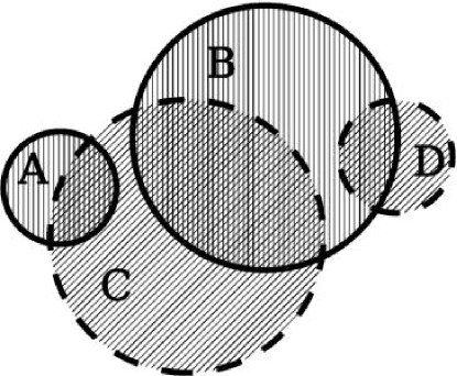
Figure 2: A pathological association case. Features A and B are in the previous frame, C and D in the current frame. A maximum-overlap method associates B and C. The recommended associative algorithm (dual-maximum overlap) associates B=C if and only if $B\cap C$ is the largest of C’s intersecting regions and also the largest of B’s intersecting regions. A and B merge to form C, at the same time that D calves via fragmentation from B.

All four of our codes follow variants of the largest-intersection criterion, either following maximum flux overlap or maximum area overlap. YAFTA uses arbitrary label choice on its first pass through the data, and then “label conflicts” in a subsequent pass that uses maximum overlap.

2.5 Filtering based on size/longevity

When working close to the noise floor, it is useful to reject small features, because false positives are much more likely in small clusters of pixels than in large ones. All of our codes reject identified features that do not meet some minimum size criterion. Criteria that are useful include: maximum size; average size; lifetime; or total number of pixels across the life of the feature. The filtering can be accomplished only after feature identification (for per-frame size checks) or feature association (for maximum size checks or longevity checks).

Additional problems exist due to fluctuations in background noise that may cause features that appear for only a single frame, or may cause weak but persistent features to disappear for a frame (the Swiss cheese problem). Similarly, associated features may split and then re-merge rapidly due to fluctuations in a single frame (the oscillating twins problem).

CURV sidesteps association problems by requiring oversampling on the time axis of the input data cube; this reduces the frame-to-frame fluctuations of individual features.

MCAT avoids both problems with a three-step process. (i) completely-surrounded holes in the center of a feature are filled in and the missing pixels are counted as part of the feature; (ii) Twin features that merge for a single frame are forced to remain separate; (iii) single features that split for a single frame are forced to remain merged.

SWAMIS overcomes both the oscillating twins and Swiss cheese problems by re-associating short lived features with nearby larger features if there is sufficient overlap between them.

2.6 Classification of Origin and Demise

Identifying and locating individual features as they evolve is properly described as feature tracking, but identifying structures and events that may include several features is more properly described as a complete computer vision application. Not all of our feature tracking codes include provision to detect and identify interactions of multiple flux concentrations, such as pairwise emergence, but such detection is an important part of characterizing magnetic evolution and hence is discussed here. In particular, because magnetic features are not corks but rather cross-sections of curvilinear manifolds (field lines that pass through the photosphere), they are connected pairwise by the magnetic field. Identifying the association between freshly emerged pairs thus gives useful information about the overall field topology and how it changes via reconnection of the overlying field before the death (e.g. by submergence) of the individual features.

The origin and demise of features is different than the origin and demise of magnetic flux itself: in particular, features can fragment or merge under the influence of the photospheric flow field (e.g. Schrijver et al. 1997) without any flux emerging or submerging through the photospheric surface. Fragmentation and merging can result in apparent violation of the conservation of flux as magnetic flux sinks below or rises above the detection threshold of the instrument being used to detect it.

Software to identify origin events recognizes flux concentrations near each newly detected concentration, and classifies the origin according to these nearby concentrations and the time derivative of their contained flux. To avoid missing associated structure, an allowed margin of error is required in the spatial or temporal offset between two associated features, and also in the flux rate-of-change between the features.

Demise events are similar to origin events and may be recognized with the same code, operating on tracked data in reverse time order. As with birth events, demise events are not necessarily related to emergence or submergence of magnetic flux.

3 Tracking Results: A Comparison Across Codes

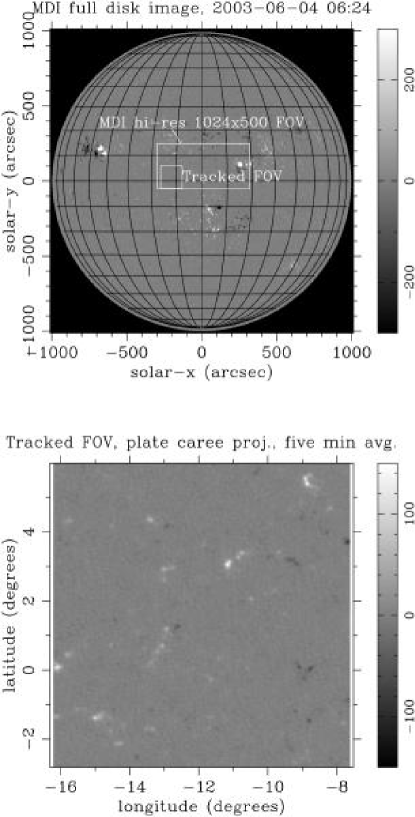
Figure 3: The tracked field of view, in context. Note that the edge of the grey circle in the MDI full-disk image is not the limb of the Sun, it is a crop radius for the instrument, just outside the limb.

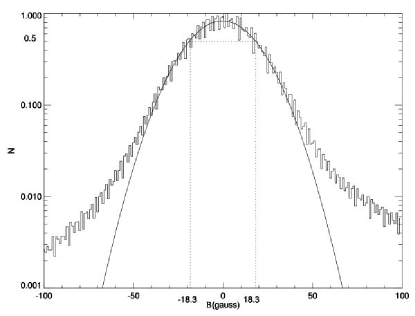
Figure 4: Distribution function of weak-field pixels in the test dataset, a sequence of five-minute average high resolution magnetograms from SOHO/MDI. A Gaussian fit to the low-valued pixels (presumed to be noise) is shown. The measured standard deviation ($\sigma$) of the images is 18.3 Gauss.

3.1 Description of the Dataset

We analyzed a sequence of 600 one-minute-cadence MDI high resolution quiet-sun images from 2003 June 04, beginning at 05:43 UT. The images were resampled into heliographic longitude/latitude coordinates (plate caree projection) using an orthographic model of the solar image, as shown in Figure 3. The reprojection used the ANA language resampling tools by R. Shine (1999, personal communication). The tracked images were 300x300 pixels and ran over the range $-16.3^{\circ}$ — $-7.3^{\circ}$ in longitude and $-2.8^{\circ}$—$6.2^{\circ}$ in latitude. This scale slightly enlarged the images, to a pixel size of 0.03 heliocentric degrees (about 0.48 observer arc seconds at disk center). Images were derotated to the central time in the data sequence, using the Snodgrass (1983) synodic differential rotation curve and rigid-body rotation at a latitude of $14^{\circ}$. These derotated, plate caree images were averaged together in blocks of five minutes each to reduce shot noise and P-mode interference. The noise level was determined by fitting a Gaussian profile to the weak portion of the pixel strength distribution curve (Figure 4). The width ($\sigma$) of the best fit Gaussian profile was 18.3 Gauss, which should be taken as the sum of all incoherent noise components (principally shot noise, granulation, and P-mode leakage). Small frame-to-frame offsets of the zero point (presumably due to variations in the instrument’s exposure time) were found by measuring the offset from zero for the best-fit Gaussian, and removed by subtraction from each frame.

3.2 Feature size distribution

The simplest comparison to make across codes is distribution of fluxes of detected magnetic features. Figure 5 shows the results of applying all four of our codes (with two different identification techniques for SWAMIS) to the same data. The five different techniques yield obviously different flux distributions for the network; here we discuss the features in the plots and the differences between them. The plots all have the same height scale and the same bin size, so the histograms are directly comparable. All the codes exhibit high and low threshold behaviors that are discussed below; but it should be immediately apparent by inspection of Figure 5 that the codes diverge at the small end of the flux spectrum, achieving a moderately good agreement in slope only for flux concentrations larger than about $2\times 10^{18}$ Mx. All four methods produce a slope of about $-0.35\pm 0.05$ decades per $10^{18}$ Mx, corresponding to an e-folding width of about $1.2\times 10^{18}$ Mx in the distribution.

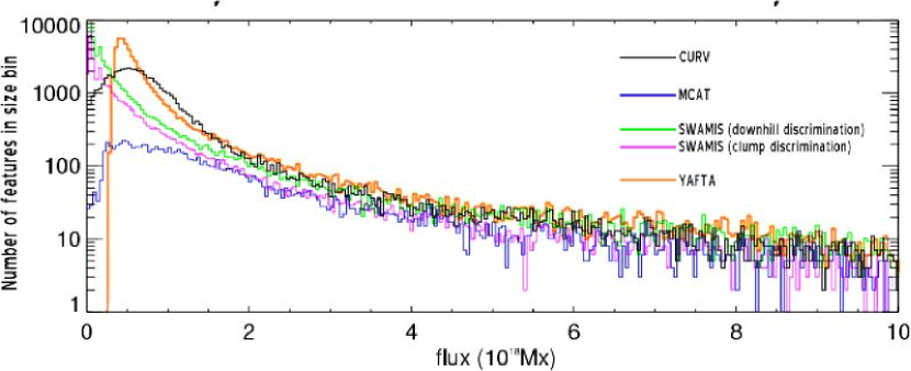
Figure 5: Network feature flux distributions as derived by the five algorithms we compared in §3. See text for full discussion.

All of the codes display a weak-feature threshold effect (false negatives) as small features that are close to the noise floor are eliminated by the discriminators. YAFTA and MCAT show the strongest threshold effects, because they rely on a combination of minimum strength and minimum feature size in each frame to eliminate false-positives from the discrimination step. The YAFTA threshold is particularly abrupt because the initial detection discriminator uses no hysteresis, so that all detected features must have a minimum number of pixels with a minimum amount of flux per pixel. MCAT’s threshold is softer because the hysteresis feature of the discriminator allows weaker pixels to be detected around a strong core; the dearth of very weak features is due to the combination lifetime-and-strength requirement, which removes many weak features that are detected by the other codes. CURV shows a still softer turnover and threshold because the CURV discriminator does not rely on a high threshold value in any one pixel to trigger detection. The turnover at about $1\times 10^{18}$ Mx reflects the geometrical factor of 3 that is applied to CURV measurements, together with the requirement for a 9-pixel concave-down region. SWAMIS shows no obvious threshold at all because its recursive temporal hysteresis admits many features that have no strong pixels in a particular frame: provided that a feature has a single strong pixel at any point in its lifetime, all of its pixels are subjected to the weaker threshold.

The disagreement between the different codes on the weak feature distribution is telling: it is difficult to distinguish reliably the flux distribution of magnetic features that are smaller than about $10^{18}$ Mx in strength even with time-averaged and conditioned MDI data. The MDI hi-res $1\ \sigma$ detection threshold in our time-averaged data is about $2.2\times 10^{16}$ Mx, corresponding to a single pixel with an 18 Gauss signal (Figure 4); features with less than $50\times$ this much flux are not reliably detected across methods.

The greater weak-feature counts of CURV and YAFTA compared with SWAMIS and MCAT do not necessarily correspond to greater sensitivity: our data set was not controlled for false positives. When characterizing a code for weak feature sensitivity, one should use noise injection null techniques to identify false positive rates. Likewise, despite the lack of obvious threshold the SWAMIS weak-feature distribution curve should not be trusted below about $1\times 10^{18}$ Mx because the hysteresis requirement may reject many transient weak features that never happen to achieve the flux density required to trip the high threshold.

In the moderate-strength feature range of $2-5\times 10^{18}$ Mx, all four of YAFTA, MCAT, SWAMIS/downhill, and SWAMIS/clump are in reasonably good agreement, with the main difference being between the downhill-like codes (CURV, YAFTA, and SWAMIS/downhill) and the clumping codes (MCAT, SWAMIS/clump). The difference is due to the segmentation of large features into several smaller ones, giving the downhill-like codes slightly more small features and slightly fewer large ones.

The different codes disagree substantially on slope of the flux distribution curve in two different regions. Below about $1\times 10^{18}$ Mx , the codes diverge strongly in feature counts and all have distribution features that might serve to indicate a transition to noise-dominated numbers: the slopes change in all the codes, and codes with thresholds of various sorts exhibit turnover behaviors due to those thresholds.

In the small-feature range $1-1.5\times 10^{18}$ Mx, each individual curve has no clear indication that the data are becoming unreliable, but the different detection schemes give divergent results. CURV and YAFTA find more small features than MCAT or SWAMIS in this range, due to a combination of noise and higher sensitivity. MCAT, which has the most stringent noise-elimination steps in the detection code, detects signifficantly fewer features in this size range, yielding a lower slope.

In the window of $\leavevmode\nobreak\ 1.5-7\times 10^{18}$ Mx, all three codes agree on the slope of $-0.28\pm 0.03\ \textrm{decade}^{-1}$, or an e-folding width of $1.55\pm 0.15\ \times\ 10^{18}$ Mx. The downhill-like methods find the steeper limit and the clumping methods find the shallower limit. Features in this size range are strong enough to be detected by all three discriminators but not so large that the differences between the large-scale behavior of the three codes is important. We conclude that features in this size range are easily detectible with MDI and results that use this feature size range are robust against small changes in detection technique.

The large-feature performance of the codes varies slightly across algorithm, though all four algorithms are in rough agreement below $10^{19}$ Mx. At higher values the feature counts are too low to provide good statistics, but general comments are possible. The CURV discriminator tends to break up large features into multiple small features, and very large features tend to have wider wings than the Gaussian profile that is assumed by CURV, slightly lowering the number of detections well above $10^{19}$ Mx. YAFTA and SWAMIS/downhill also tend to break up very large concentrations of flux into multiple features, but that effect is not as strongly apparent. SWAMIS/clump and YAFTA agree quite well on the flux distribution from the YAFTA threshold to several $\times 10^{19}$Mx. In this size range, results appear reproducible but care is needed when inferring physical values from tracking results as the results appear dependent on the method used to identify individual features.

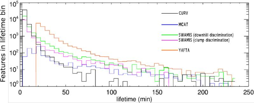
Figure 6: Measured feature lifetime is strongly dependent on tracking technique, as seen by comparing lifetime histograms derived from each of the authors’ separate tracking codes. See text for full discussion.

3.3 Feature Lifetimes

Feature lifetime is strongly affected by the feature-association step of the codes and hence cross-code comparison is important to identify how reproducible that step is. Feature lifetime is also important to the solar physics: it is used as important measure of flux turnover rate (e.g. Hagenaar et al. (2003)), although some physical effects other than flux turnover can affect it. By comparing our codes we obtain a measure of the reliability of feature lifetime measurements in the literature.

Several potential effects can introduce errors into flux turnover rates measured with feature tracking codes. In particular, fragmentations and mergers of like-signed features cause end-of-life events, while the associated magnetic flux survives. Similarly, fluctuations in the total flux or the area of a small feature cause many birth and death events. These effects tend to shorten the measured lifespan of features, causing an apparent (but not real) increase in the turnover rate of magnetic flux.

Similarly, all of our codes observe many features that are born and/or die in a way that does not apparently conserve magnetic flux; these events may be due to asymmetries in the field strength of small bipoles, or due to statistical fluctuation in a collection of very small, unresolved concentrations of magnetic flux. If the latter is true, then the individual unresolved concentrations that make up a feature must have much shorter lifespans than the resolvable feature, causing an apparent (but not real) decrease in the turnover rate of magnetic flux.

Figure 6 shows a histogram plot of feature lifetime from each of our codes. The codes agree on the slope (but not the value) of the lifetime histogram for a narrow range of lifetimes between 20-50 minutes. Roughly 75% of features found by SWAMIS in this range of lifetimes are in the $2-6\times 10^{18}$ Mx size range in which the codes agree on feature counts, suggesting that this region of slope agreement is similar to the region along the size axis: features in this population are high enough above the noise floor to be readily detectible but not so large nor long-lived that geometrical effects fool the different tracking algorithms.

The differences between the curves are entirely due to differences in the algorithms of the codes, as we examined identical data. MCAT requires longevity of more than two frames (10 minutes) in the identification step; the small number of one-frame features are due to fragmentations (features that fragment from an existing feature, then disappear one frame later). SWAMIS and CURV use much weaker longevity requirements, and therefore detect similar numbers of short-lived features. YAFTA detects many more short-lived features than the other codes, in part because of a lower detection threshold (no detection hysteresis was used for this data set) but does not include any features with less than a 4-frame (20 minute) lifetime.

CURV, alone of all the codes, shows a minimum in the lifetime histogram followed by a slight rise in the 150-200 minute range. The population in the rise consists of nearly 100 structures, enough to be statistically significant compared to just 9 features features found by CURV in this data set with lifetimes between 100 and 150 minutes. It is not clear whether this is an unusual statistical event or a quirk of the CURV association scheme.

The main conclusion to draw from this comparison is that feature lifetimes are extremely difficult to measure with tracking codes; in consequence, average magnetic lifetime results from magnetic tracking of arcsecond-scale data should be considered weak. We will address the nuances of lifetime measurement, and its relevance to physical parameters such as magnetic turnover time and heating rate, in a later article in this series.

4 Discussion

Each of the techniques we considered has advantages for a particular regime of fragment size and strength relative to the noise floor of the instrument. Here, we discuss the tradeoffs of the different detection schemes. The main differences between our codes lay in the discrimination and feature-identification steps, which are discussed separately.

4.1 Discrimination

The main problem faced by tracking discriminators is the huge number of statistically independent samples across an image sequence dataset. The simplest discriminator is a threshold trigger; while threshold triggers are inadequate for many tasks when used alone, they form the basis of every discrimination algorithm. The three main ways we improved upon simple threshold triggering were curvature sensing (CURV), hysteresis (MCAT, SWAMIS), and post-discrimination filtering for feature size and longevity (all codes). Simple trigger discrimination is useful mainly where the signal-to-noise ratio is overwhelmingly large. One code in our study (YAFTA) was optimized for strong field detections and used simple trigger discrimination, although subsequent versions of YAFTA include the ability to use hysteresis.

Curvature sensing as implemented in CURV has the advantage that, when combined with a threshold trigger, it applies five statistically independent threshold tests to each pixel, significantly reducing the false-positive rate. CURV rejects features whose convex cores are smaller than 9 pixels. Including the effects of smoothing in the preprocessing steps, which leave granulation as the dominant source of noise, there are about 12 statistically independent tests (of 45 total conditions) required to detect a particular feature. By contrast, a direct trigger yields only about three statistically independent tests with the same size threshold. Curvature discrimination permits a detection threshold much closer to the noise floor than would otherwise be possible, which in turn should make curvature discrimination rather sensitive to weak concentrations of magnetic flux.

The disadvantage of curvature discrimination is that it only finds the convex core of a magnetic feature. This is addressed by Hagenaar et al. (1999) via a simple scaling: they find that for a large variety of near-Gaussian distributions the convex core is about 1/3 of the total flux in the feature, and scale accordingly. This works well for small features near the resolution limit of the observations, but not as well for larger features, which are observed to have flatter profiles than a Gaussian. Large concentrations of flux typically have several local maxima, and the total flux may be over- or underestimated by the assumption of a simple Gaussian shape, depending on the actual morphology of the feature.

Hysteresis is a simple way of reducing the false positive rate of threshold-trigger discrimination. Pixels are compared against different trigger thresholds depending on whether they are isolated or adjacent to other detected pixels. Both MCAT and SWAMIS use a recursive-hysteresis scheme that starts with a simple threshold scheme, and then dilates detected pixels using a lower threshold. Such schemes eliminate many false positives due to the background noise floor, and detect the full extent and shape of large features. The drawback is that weak features are only detected if they have at least one ’seed’ pixel that is stronger than the high threshold. SWAMIS further allows dilation along the time axis, so that weak features are detected if at some point in their lifetime they have a single strong pixel; but even so, many transient weak features that are visible to the eye go undetected for lack of a single strong pixel.

4.2 Feature Identification

Here, we contrast the two principal dilation strategies of the codes: downhill and clumping dilation from local maxima. The distinction between these strategies is academic within CURV, as the curvature-based discriminator provides well-separated loci around each local maximum: the final detected loci are the same regardless of dilation method. MCAT, SWAMIS, and YAFTA can dilate using clumping, and SWAMIS and YAFTA can dilate using the downhill technique.

Both the downhill and clumping techniques, together with hysteretic thresholding, do better than curvature at identifying the size and shape of mid-sized magnetic features in the several arc second size range. In this size range the shape of individual features varies considerably, though most features still have but one local maximum in the MDI data that we tracked; under these conditions, both dilation techniques do about as well as one another and both measure the flux of individual features with more precision than CURV (which uses a simple geometric factor to estimate the flux in the wings of the structure).

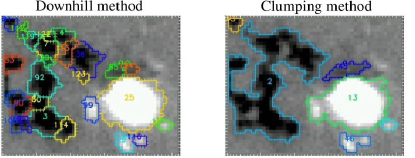
Figure 7: Effect of feature identification technique: a pathological case. Clumping (right) is less sensitive to noise in weak features than is downhill dilation (left), but can lead to counterintuitive results in active regions as large, irregular patches of flux are identified as a single object.

Large scale structures that are more than about 15 arc seconds across yield stronger differences between the downhill and clumping techniques, as illustrated in Figure 7. The downhill technique does a better job at tracking substructure of large, extended objects such as plage and active region fields, but at the expense of more noise susceptibility. Because small amounts of noise can produce transient local maxima in a large extended feature, the downhill technique is susceptible to the swiss cheese problem in which a single large clump of flux with no strong local maximum can be oscillate between being detected as one or several separate features. If lifetime filtering is being applied to the detected-feature list, then large holes may appear in the detected feature, giving it the appearance of an irregular block of Ementhaler cheese. Furthermore, downhill detection alone tends to miss very large concentrations of flux, treating them as a collection of smaller features: while this is desirable for tracking the motion of the solar surface, it is not desirable when measuring the statistics of strength or size of magnetic features.

We discuss the tradeoff between these detection techniques, neither of which is perfect, in §5, below.

4.3 Cross-frame feature association

All of the codes we compared use essentially the same cross-frame association strategy of finding the association map that maximizes overlap between features in adjacent frames, as described in §2.4. In practice, most features in most frames overlap with exactly one feature in the following and adjacent frames, so variations in the type of overlap (e.g. number of pixels vs. amount of flux) or of permissiveness of overlap (e.g. including pixels nearby each feature as part of the feature itself, for purposes of finding overlap) only affect the “edge cases” in which multiple magnetic features are interacting, or in which a single feature is moving rapidly.

Overlap-style algorithms such as described in §2.4 are quite robust for associating features with the properties $\forall i,j:\left|\overrightarrow{x_{i}}-\overrightarrow{x_{j}}\right|\gtrsim r_{i}$ and $\forall i:\left|\Delta\overrightarrow{x_{i}}\right|\lesssim r_{i}/2$, where $i$ and $j$ are indices across features, $\overrightarrow{x_{i}}$ is the centroid location of feature $i$, $r_{i}$ is the typical radius of feature $i$, and $\overrightarrow{\Delta x_{i}}$ is the displacement vector of feature $i$ across frames. Fast moving features with $\left|\Delta\overrightarrow{x_{i}}\right|\gtrsim r_{i}/2$ become subject to the mistaken identity problem, where they are identified as a different feature in different frames. The mistaken identity problem affects statistical feature-lifetime and feature history results even if only a very few features are subject to it, because a single fast-moving feature may register as a very large number of separate magnetic features. The only reliable way to beat the mistaken identity problem is to use high enough time resolution in the data. Marginal data in which the fastest moving features have $\Delta\overrightarrow{x_{i}}\thickapprox r_{i}$ may be improved by interpolating interstitial frames, but wider separations cannot be helped by that method. In practice, we found by visual inspection that 12-minute final effective cadence with direct boxcar averaging was not sufficient to avoid the mistaken identity problem for the fastest moving features at the MDI “full disk” resolution (1.4 Mm pixels at Sun center), accounting for ~0.5% of features in a given frame and perhaps 5% of total features identified by SWAMIS, but that 12 minute final effective cadence with anti-aliasing in the time direction (time-weighted averaging of 1 minute cadence magnetograms, with a 12 minute FWHM Gaussian weighting profile) eliminates virtually all cases of mistaken identity.

We considered, but did not implement, various methods to reduce the mistaken identity problem in cases where high enough cadence data are not available. Promising directions to try include linear extrapolation of feature location from last associated location before the overlap calculation, with or without backtracking on the time axis; dilation with size checking; and simulated annealing of feature association. We suspect that all such algorithms are likely to include more faulty associations than does direct overlap.

5 Recommendations on Accepted Practice

To enable meaningful comparison and reproducibility of tracking results across research groups, we recommend the following techniques as appropriate for most applications of magnetic feature tracking.

5.1 Data preprocessing

While preprocessing of data is not technically a part of feature tracking, preprocessing can affect the statistics of image tracking and therefore warrants mention here. We discuss despiking, time averaging, and resampling into a desired coordinate system.

Despiking

A brief note on space-based magnetograms is in order: SOHO/MDI is, and presumably SDO/HMI will be, susceptible to cosmic ray impacts. A typical MDI “full-disk” magnetogram has evidence of cosmic ray impacts in $\leavevmode\nobreak\ 10^{2}$ pixels, so 5-10 minute averages may have as many as $\leavevmode\nobreak\ 10^{3}$ bad pixels caused by cosmic rays. The cosmic rays are not saturated in the images, and may have either negative-going or positive-going direction. These cosmic rays can skew the size, strength, and lifetime statistics of small, short-lived features if not considered. We recommend either despiking sequences of space-based magnetograms with a second time derivative technique such as ZSPIKE (DeForest 2004), or imposing a lifetime threshold on detected features to limit the effects of cosmic rays.

Time and spatial averaging

Time averaging of images is useful as a preparatory step to reduce noise in the magnetograms and to smooth features for better association across frames. There are several sources of noise in currently available magnetograms, with different statistics for each source; we discuss them briefly here, as the noise characteristics of averaged data sets hold a complex relationship to the noise characteristics of individual frames.

Most magnetographs are photon-limited, so that there is an approximately Gaussian distribution noise source of photon noise associated with photon counting statistics in each pixel of each magnetogram. Each pixel contains an independent sample of this noise source. Magnetographs such as MDI that assemble multiple exposures are subject to shutter noise, which results from very slightly different exposure times across each independent exposure used to produce the magnetogram: shutter noise is an approximately Gaussian distribution noise source that is added to the common mode of all pixels across each image. Finally, solar evolution (and, for ground-based telescopes, seeing effects) across the time of assembly of the magnetogram induces an additional noise source, evolution noise that is dominated by the evolution of granules. Granulation, and the associated evolution noise, has about one independent sample every five minutes, per square megameter of solar surface area.

Individual MDI magnetograms have about equal amounts of photon and evolution noise. Because the photon noise is independently sampled in each image, averages of more than about five minutes of magnetic data tend to be dominated by evolution noise, which is attenuated much more slowly by further averaging.

Anti-aliased time averaging, using overlapping Gaussian or Hanning windows in the time domain, is preferable to simple boxcar averaging, which has frequency sidelobes that allow more noise to enter the data.

Image resampling

Image sequences are typically resampled to remove the solar rotation and perspective a priori. For the present work, we derotated and prepared time averages of MDI magnetograms using a simple interpolation scheme into plate caree coordinates. This scheme follows current common practice but is not recommended: it fails to preserve small-scale feature statistics in two important ways.

First, the plate caree (“lon/lat”) map projection is non-authalic: a feature of unit area on the surface of the Sun may have different areas in plate caree coordinates, depending on its latitude. To avoid skewing the statistics of flux content, authors should use an authalic (equal-area) projection to prepare the data before tracking. The area of a feature in the plate caree projection is scaled by a factor of secant(latitude). A simple way to compensate is to scale the vertical or horizontal scale by cos(latitude) at each point. Scaling the vertical axis by cos(latitude) yields the common sin-lat cylindrical projection, so named because integrating the scale factor $y^{\prime}_{map}\leavevmode\nobreak\ cos(lat)$ yields $y_{map}\leavevmode\nobreak\ sin(lat)$. Scaling the horizontal axis yields the sinusoidal projection. Other useful authalic choices include the Hammer/Aitoff elliptical projection used by the cosmology community and Lambert’s azimuthal equal-area projection, which minimizes linear distortion near the origin. Many useful projections have been cataloged by Snyder (1987).

Secondly, linear interpolation leaves much to be desired as a resampling method, skewing (among other things) the noise profile of individual pixels and potentially introducing large amounts of distortion into the statistics of small features. A statistically sound, photometrically accurate resampling method, relying on spatially variable sampling filters, has been described by DeForest (2004); that or similar techniques are recommended for preparing data for survey applications.

For virtually every application of tracking, it is important to compensate by rigid rotation based on the differential rotation speed at a particular point in the field of view, and not by differentially rotating every pixel in the image independently. The former preserves the actual evolving spatial structures in question; the latter only preserves the plasma reference frame at the start of the observing run.

5.2 Feature discrimination & identification

We recommend combining the three methods of feature detection. Standard codes should use a dual-discriminator scheme for detection: an initial convex-core discrimination as in CURV, followed by dilation to a low noise threshold. This combination takes best advantage of the extra discrimination afforded by the convex core technique, while eliminating some of the difficulties of identifying oddly-shaped and large features.

Feature identification should use the downhill method to avoid pathologies of the clumping technique, particularly when used for motion tracking and to identify interacting magnetic features; but for applications where larger clusters of flux are important, we recommend keeping track of groups of touching or nearby features according to a clumping algorithm. Groups of mutually touching features are the same loci as would be identified by a direct clumping scheme, but tracking individual peaks within the group affords better localization of the magnetic flux that makes up the feature(s). This can be accomplished either by maintaining a table of mutually touching features or by using a dual-labeling scheme at the feature-identification step.

5.3 Feature association

For best general purpose utility, we recommend a flux-weighted maximum overlap method of association between frames, as is currently used by SWAMIS; for example, in cases of associative conflict such as Figure 2, regions B and C would be associated as identical, region A would be classified as dying by merger into B/C, and region D would be classified as originating by fragmentation from B/C. For analyses that require feature identification, it is important to ensure that the cadence is sufficient to allow associated features in adjacent frames to overlap. While more sophisticated motion-correlation algorithms are in principle feasible, they add complexity and fallibility that is not necessary provided that the data have high enough cadence.

It is notable that no local overlap algorithm agrees with a human observer in all cases, as human observers use more information than strict overlap – including something like a predictor/corrector position algorithm. Maximum overlap works well in the case where the motion of all features is small compared to their width divided by the time step. If the time step is too long, small features can move more than their diameter in a single frame, leading to the mistaken identity problem, where a single visually identifiable feature frequently changes its identity in the tracked data. In such cases, one can (i) use faster frame rates, (ii) generate dilated feature masks for association, (iii) use linear location extrapolation to account for the large interframe motion, and/or (iv) use a minimum-distance criterion rather than maximum overlap.

5.4 Feature tabulation

When tabulating feature histories, we recommend that the following minimum information be kept for each feature, and for each frame for which a particular feature exists: area (A), total flux ($\Phi$), flux-weighted average location (x,y), and flux-weighted quadrupole moments ($<\Phi^{2}dx^{2}>,<\Phi^{2}dy^{2}>,<\Phi^{2}dxdy>$), for a total of 7 numerical quantities per feature per frame. The quadrupole moments, in particular, summarize tersely and simply the shape of the feature, and the features detected by the downhill dilation method tend to be simple shapes that are readily described with the quadrupole moment set. Quantities may be kept in physical or image units (e.g. km or pixels). Quantities which we recommend avoiding are: pixel value maximum and variance, which depend on resolution and phase of the underlying feature relative to the pixel grid; and non-weighted average location, because it is more dependent on noise-dominated pixels at the feature’s edge than is the flux-weighted average location.

5.5 Event identification

Several of the scientific applications of tracking require classifying the origin and demise of each feature based on visual heuristics for the underlying physics. Useful event classification requires characterizing the geometry and manner of change of nearby features. Event classification is a rich topic that is not fully discussed in this paper; however, we make some brief recommendations.

We recommend classifying origin events into four categories: (i) isolated appearance, in which a particular feature appears in the absence of interaction with surrounding detected features; (ii) balanced emergence, in which a bipolar, approximately balanced pair of features appear together in nearly the same location at nearly the same time; (iii) unbalanced emergence, in which a new feature appears next to a pre-existing, opposite sign feature in a nearly flux-conserving manner; and (iv) fragmentation (or splitting), in which a single pre-existing feature breaks up into multiple smaller features in a nearly flux-conserving manner. Demise events should be classified in the exact same way as origin events, in a time reversed sense: (i) isolated disappearance; (ii) balanced cancellation; (iii) unbalanced cancellation; and (iv) merging. For both origin and demise events, (i) is the only recognized case that apparently violates conservation of flux; (ii) corresponds to isolated passage through the photosphere of a magnetic loop; and (iv) represents reshuffling of existing flux. For completeness, event identification software should also maintain a complex class for events which cannot be classified easily into the above four groups, including such events as isolated asymmetric emergence that violate conservation of magnetic flux.

It is important to understand that this is a visual classification scheme, to be more fully developed in future work. Interpretation of these visual events in terms of physical mechanisms is neither straightforward nor obvious. For example, appearance events may or may not correspond to new flux on the solar surface.

Physical modeling of feature behavior requires some care. In particular, only some emergence events (bipolar emergence) appear to be due to flux tubes that emerge from below the surface of the Sun (Harvey and Martin 1973; Harvey 1993; Chae et al. 2001). Such events should give rise to two oppositely signed magnetic features that grow together and separate in a divergent surface flow (Hagenaar 2001; Hagenaar et al. 2003; Simon et al. 2001), and the origin detection code in SWAMIS and in CURV was originally intended to identify such events. However, proportionally few magnetic features are observed to originate with this balanced emergence mechanism. New small features can also form by fragmentation of pre-existing large features into like-signed fragments; this process is also called calving if the new feature is small compared to the surviving feature. Furthermore, many features simply appear, without any surrounding flux at all or in ways that appear to violate flux conservation. The nature of these appearances – whether coalescence of existing weak flux or unbalanced emergence with one large, weak-field pole and one small, strong-field pole, will be considered in detail in Paper II of this series.

Results using our recommended classification scheme should be presented together with a notation describing what criteria are used to detect balanced changes in the flux of interacting features. Event classification results can be quite different, for example, if the changes in the flux of two interacting features are considered “approximately balanced” if they merely have opposite sign, or if they must agree within, say, 10%.

6 Conclusions

We have compared four magnetic feature tracking codes by applying them to the same preprocessed set of magnetic data. Feature tracking code output is sensitive to a variety of decisions that are made during development, and this sensitivity is a reason why it has historically been difficult to reproduce results obtained by feature tracking: it is crucial to explain exactly what algorithm is being used. In particular, codes that were designed for one regime of study (e.g. very small intranetwork flux concentrations or very large, strong features) should not be applied to different regimes of detection without careful study, and all discrimination and association techniques need to be lain out exactly as performed.

The difficulty of reproducing apparently simple results in feature tracking appears to stem both from the complicated, noisy nature of the magnetograph data and from the complexity of the underlying structures. The solar magnetic field is not divided into well separated, strongly magnetized features; rather, there is a continuum of feature sizes due to the clustering behavior of the field across scales, in keeping with the concept of magnetochemistry outlined by Schrijver et al. (1997). Bulk summary characteristics such as the lifetime of individual features or the size distribution of the features depend strongly both on the instrument being used to image the magnetic field and on threshold and related decisions made during code development.

All of our codes agree reasonably well on important summary characteristics in a particular circumscribed range of scales and lifetimes, indicating that there is an underlying pattern to be measured; but the region of agreement (which we take to be the range of valid measurement using the tracking codes) is much smaller than might be surmised from cursory analysis of the output of any one algorithm. We conclude that particular care must be used when interpreting magnetic tracking results, which are often much weaker than might be surmised given the apparent clarity of solar magnetic features in magnetogram sequences.

In particular, we find that the magnetic turnover time, perhaps the most accessible summary result to come out of magnetic tracking studies, is also perhaps the weakest result to come out of magnetic tracking studies. Average feature lifetimes are only weakly related to magnetic turnover time in the best of circumstances, and we have found that average lifetime measurements are strongly dependent on the code being used to perform the measurement.

By comparing and contrasting the algorithms of our four separate codes, we have determined why the they produce different results for the flux distribution in quiet sun, and evaluated under what circumstances each technique performs best. Further, we have made recommendations about how to improve feature detection and reproducibility in feature tracking for future work. To aid that work, all four of our codes are being made available to the scientific community in source-code form via solarsoft.

Specific physical problems such as flux emergence and cancellation, diffusion of active region flux and plage formation, and feature lifetime, will be covered in more detail in future papers in this series.

Glossary

Feature tracking and magnetic observations are mature enough to have developed a collection of commonly used terms, which unfortunately have drifted into slightly different usage in different locations. In an attempt to regularize terminology, we present a glossary of commonly used terms, with their recommended definitions. Also, because some terms are strictly observational and others imply a physical model, we have noted which are which.

Object descriptions

bipole

- a pair of magnetic features of opposite sign and approximately equal flux content, that appear to be associated (as in bipolar emergence). When seen to emerge together, the poles of a bipole may be associated observationally.

ephemeral region

- a resolved small bipole with particular properties as described by Hagenaar [2001].

feature

- a visually identifiable part of an image, such as a clump of magnetic flux or a blob in a magnetogram. The term “feature” is purely observational and is preferable to “flux concentration” or “ephemeral region” when describing individual visual objects in an image. The specific definition of a feature is dependent on both the Sun itself and the characteristics of the observing telescope.

flux concentration

- a localized cluster of magnetic flux, with or without resolved substructure. A flux concentration may consist of one or more magnetic features. While somewhat vague, the definition of a flux concentration is approximately independent of observing telescope: a flux concentration may appear as a single feature when seen with one instrument but as several features with another.

fragment

- a small piece of a larger magnetic structure, not a generic small bit of magnetic flux. Usage: “this magnetic flux concentration is composed of many fragments”, or “unresolved fragments make up this magnetic feature”. “Fragment” should not be used interchangeably with “feature”, as it implies that the subject is part of a larger whole, while “feature” does not.

monopole

- a lone magnetic pole (thought to be physically impossible).

stenflo

- (after J. Stenflo) a tiny, strong concentration of order $10^{17}$ Mx of flux. Usage: “The asymmetric formation of flux concentrations in the network may be due to convergence of stenflos, though Stenflo himself may object to this terminology.”

unipole

- a single magnetic feature with no obvious associated feature of the opposite sign. The photospheric boundary provides a “hiding place” for the opposing pole, so that unipoles are thought not to be monopoles. Oppose “bipole”, “monopole”.

Event descriptions

appearance

- used specifically to describe the origin of a single unipolar feature where there were none before. Appearances appear to violate conservation of magnetic flux, but probably result from flux hiding under the noise floor of an instrument – so the definition of “appearance” depends on the instrument being used.

asymmetric emergence

- emergence in which the two sides of the emerging magnetic loop of flux have quite different cross sections, perhaps reducing the field strength of the larger leg of the loop below the detection threshold of an instrument. This can be a physical description of one type of feature appearance; coalescence is another type. Note that “asymmetric emergence” and “unbalanced emergence” are not synonyms.

balanced emergence

- emergence in which the two final opposing-sign features have approximately the same magnitude; this is the type of emergence predicted by a simple model of magnetic flux tubes rising through the photosphere. Compare “emergence”; contrast “unbalanced emergence”.

balanced cancellation

- cancellation in which the two initial opposing-sign features have approximately the same magnitude. Compare “cancellation”; contrast “unbalanced cancellation”. Balanced cancellation is the time reversal of balanced emergence.

calving

- a form of fragmentation in which one of the daughter features contains much more flux than the other, by analogy to the behavior of icebergs. Usage: “This movie shows small features calving off of the main flux concentration”. Oppose “splitting”; compare “fragmentation”.

cancellation

- the demise of a magnetic feature that collides (and cancels) with an opposing sign feature, in such a way that flux is approximately conserved. Compare “balanced cancellation”, “unbalanced cancellation”; contrast “disappearance”.

coalescence

- the collection of diffuse flux from below detection threshold to a small, denser feature that can be detected. This may be an example of unresolved merging. This is a physical description of one type of feature appearance; asymmetric emergence is another type. To avoid confusion, eschew “coalescence” when describing observational results; use “merging” or “appearance” instead.

demise

- the end of a magnetic feature’s existence.

disappearance

- the end of a single, unipolar magnetic feature that “fades away” to nothing in the absence of nearby features (the time reversal of an “appearance”).

dispersal

- deprecated. This has been used to describe the opposite of coalescence, the breakup of strong flux concentrations into many fragments, and the diffusion of flux across the surface of the Sun. It is now too ambiguous to be used clearly in most cases.

emergence

- the origination of two balanced, opposing magnetic features nearby one another in such a way that flux is approximately conserved. This observational definition follows the common physical definition of a loop of flux emerging from below the surface. Compare “balanced emergence”, “unbalanced emergence”; contrast “appearance”. Emergence is the time reversal of “cancellation”.

fragmentation

- the breakup of a single magnetic feature into at least two like-sign features. (compare “splitting”, “calving”)

merging

- the joining of two magnetic features of similar sign into a single larger feature.

splitting

- the breakup of a single magnetic feature into at least two like-sign features, with the implication of rough flux balance between the two daughter features. (oppose “calving”; compare “fragmentation”).

unbalanced emergence

- emergence in which the two final opposing-sign features have different magnitudes due to interaction with a nearby unipolar feature. Compare “emergence”; contrast “fragmentation”, “balanced emergence”. Unbalanced emergence is the time-reversal of unbalanced cancellation.

unbalanced cancellation

- cancellation that is not complete because one of the canceling features contains more flux than the other. Compare “cancellation”; contrast “merging”, “balanced cancellation”.

References

- Chae et al. [2001] Chae, J. et al. 2001, ApJ, 548, 497
- DeForest [2004] DeForest, C. E. 2004, Sol. Phys., 219, 3
- DeForest and Lamb [2004] DeForest, C. E. and Lamb, D. A. 2004, BAAS, 204
- DeForest [2004] DeForest, C. E. 2004, ApJ, 617, L89
- Fossum and Carlsson [2004] Fossum, A. and Carlsson, M. 2004, ESA SP-547, 125
- Hagenaar [2001] Hagenaar, H. J. 2001, ApJ, 555, 448
- Hagenaar et al. [1999] Hagenaar H. J. et al. 1999, ApJ, 511, 932
- Hagenaar et al. [2003] Hagenaar, H. J. , Schrijver, C. J., and Title, A. M. ApJ, 584, 1107
- Handy et al. [1999] Handy, B. N. et al. 1999 Sol. Phys., 187, 229
- Harvey [1993] Harvey, K. L. 1993 Ph.D. Thesis, Univ. of Utrecht
- Harvey and Martin [1973] Harvey, K. L., and Martin, S. F. 1973, Sol. Phys., 32, 389
- Lamb and Deforest [2003] Lamb, D. A. and Deforest, C. E. 2003, AGU FMA, B530
- Leibacher [1995] LeibacherJ. W. et al. 1995, ASP Conf. Ser., 76, 381
- Leibacher [1999] Leibacher, J. W. 1999, Adv. Sp. Res., 24, 173
- Parker [1988] Parker, E. N. 1988, ApJ, 330, 474
- Parnell [2002] Parnell, C. E. 2002, MNRAS, 335, 389
- Parnell and Jupp [2000] Parnell, C. E. and Jupp, P. E 2000, ApJ, 529, 554
- Scherrer et al. [1995] Scherrer, P. H. et al. 1995, Sol. Phys., 162, 129
- Schrijver et al. [1997] Schrijver C. J. et al. 1997, ApJ, 487, 424
- Schwer et al. [2002] Schwer, K. et al. 2002, AGU FMA, C1
- Simmons [1972] Simmons, G. F. 1972, McGraw-Hill
- Simon et al. [2001] Simon, G. W., Title, A. M., and Weiss, N. O. 2001, ApJ, 561, 427
- Snodgrass [1983] SnodgrassH. B. 1983, ApJ, 270, 288
- Snyder [1987] Snyder, J. P. 1987, USGS Prof. Papers, 1395
- Strous et al. [1996] Strous, L. H. et al. 1996, A&A, 306, 947
- Welsch and Longcope [2002] Welsch, B. T. and Longcope,D. W. 2002, ESA SP-505, 611
- Welsch and Longcope [2003] ———–. 2003, ApJ, 588, 620
- Welsch et al. [2004] Welsch, B. T. et al. 2004, ApJ, 610, 1148