The Complexity of Simple Stochastic Games

Abstract

In this paper we survey the computational time complexity of assorted simple stochastic game problems, and we give an overview of the best known algorithms associated with each problem.

1 Introduction

A simple stochastic game $\mathrm{G=(V,E)}$ is a directed graph whose vertices are partitioned into four disjoint sets $V_{max}$, $V_{min}$, $V_{avg}$ and $V_{sink}$. Depending on the set a vertex belongs to, it is called max, min, average and sink vertex, respectively. In addition, one of the vertices in $V$ is given the property of being the start vertex. $V_{sink}$ contains exactly two vertices, called the 1-sink and the 0-sink. The 1-sink and the 0-sink have no children, while all other vertices have exactly two distinct children. Loop edges $e=(i,i)$ are allowed. In the rest of this paper we assume w.l.o.g. that $V=\{1,\ldots,n\}$ where $n-1$ is the 0-sink and $n$ is the 1-sink.

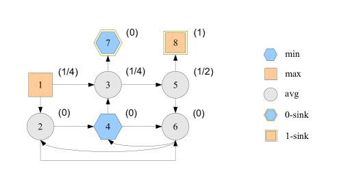
Figure 1: A simple stochastic game with 8 vertices. Vertex 1 is the start vertex. The numbers in parentheses denote the optimal vertex values.

The game is played by two players, called the max player and the min player, who have diametrically opposed objectives. At the start of the game, a token is placed on the start vertex. In each round, the token is moved from a vertex to one of its children obeying the following rule: whenever the token is positioned on a max vertex, the max player decides to which child the token is moved; whenever the token is positioned on a min vertex, the min player decides to which child the token is moved and whenever the token is positioned on an average vertex, the token is moved with probability $1/2$ to one of its children. Average vertices hence model randomness in this kind of stochastic game. The game ends, when the token reaches a sink vertex. The max player wins the game, if the token reaches the 1-sink. The min player wins the game in all other cases – that is either when the token reaches the 0-sink or when he can force an infinite play where the token reaches neither sink vertex.

The optimal value of a vertex is defined as the probability that the max player wins the game starting at that vertex, assuming both players employ optimal strategies (a strategy is optimal, if the probability of winning the game with it is greater or equal to that of any other strategy, regardless of the strategy chosen by the opponent). We will later see that both players of a simple stochastic game posses optimal strategies, albeit not unique ones. The value of the game is defined to be the optimal value of its start vertex, and the optimal value vector of the game is defined to be the vector whose components are the optimal vertex values of the game.

The most intriguing question to be asked about a simple stochastic game is: what is its value? As we shall see later, the complexity of the associated function problem is polynomial-time equivalent to that of finding the optimal value vector of the game. The problem of computing the optimal value vector of a simple stochastic game has been studied extensively from an algorithmic point of view [5, 15, 2, 11, 12, 16] (no polynomial time algorithm has been found), but the author is not aware of any previous efforts in studying its complexity. Therefore, we shall prove containment of the problem in FNP in a subsequent section of this paper.

The question about a simple stochastic game’s value is not only intriguing, it has also pratical relevance. This is because stochastic games are nowadays used as a formal tool in a variety of different application areas, including automated software verification and controler optimization, where the game’s value constitutes the single most crucial information. Apart from this, there exist some other motivations behind the study of simple stochastic games. Most of these are related to the SSG-VALUE problem – given a simple stochastic game, is its value greater than $1/2$? Though Condon [4] was able to show that the SSG-VALUE problem is contained in $NP\cap coNP$, despite significant efforts [9, 8, 2] to obtain a hardness result for a specific complexity class, the problem’s exact complexity status is unknown. Thus one of the motivations behind the study of simple stochastic games is the desire to find a complexity class for which SSG-VALUE is complete, so as to obtain a clue whether the problem is intractable or not. The present consensus is that, since contained in $NP\cap coNP$, SSG-VALUE is very likely not NP-complete and may allow for more efficient algorithms than the exponential ones currently known. Condon reinforces this hypothesis by stating that SSG-VALUE constitutes one of the rare combinatorial problems to be contained in $NP\cap coNP$, but for which containment also in P is an open question.

A last motivation behind the study of simple stochastic games can be expressed as the “kill two birds with one stone” factor; many computational problems, such as the generalized linear complementarity problem (GLCP) and the minimum stable circuit problem for min/max/avg-circuits (STABLE-CIRCUIT), were shown [8, 9] to be polynomial-time reducible to SSG-VALUE – hence more efficient algorithms for SSG-VALUE will also yield more efficient algorithms for those other problems. The rest of this paper is organized as follows: in section 2, we will restate the essential definitions for simple stochastic games as given in Condon’s initial paper on the subject. In section 3, we will provide a more detailed view of simple stochastic games which will enable us to conduct our complexity survey in section 4. The paper concludes with a summary of the important points and an overview of open problems in section 5.

2 Definitions

2.1 Player Strategies

Given a simple stochastic game, a strategy $\tau$ for the min player (or min strategy) is a subset of the game’s edges such that for each min vertex $i$ with children $j$ and $k$, either $(i,j)\in\tau$ or $(i,k)\in\tau$ applies. Substituting $\tau$ with $\sigma$ and min with max in the above sentence, we obtain the analog definition for the max strategy $\sigma$. Informally, a strategy denotes the player’s choice to which child the token is to be moved whenever it is positioned on a vertex belonging to that player. The reason for defining player strategies like this will be explained in the next section of this paper.

2.2 Reduced Games

Given a simple stochastic game $G=(V,E)$ and a strategy $\tau$ to be employed by the min player, the reduced game $G_{\tau}$ is defined to be the sub-graph of $G$ obtained by removing all edges from $G$ that are not selected by the min strategy $\tau$, i. e.

$$G_{\tau}=(V,E_{\tau})\quad\text{where}\quad E_{\tau}=E\setminus\{(i,j)\in E:i\in V_{min}\wedge(i,j)\notin\tau\}$$

$G_{\tau}$ can be regarded as the 1-player equivalent of $G$, where it is certain that the min player employs $\tau$. In a similar manner, the reduced games $G_{\sigma}$ and $G_{\tau,\sigma}$ are defined as

$$G_{\sigma}=(V,E_{\sigma})\quad\text{where}\quad E_{\sigma}=E\setminus\{(i,j)\in E:i\in V_{max}\wedge(i,j)\notin\sigma\}$$

$$G_{\tau,\sigma}=(V,E_{\tau,\sigma})\quad\text{where}\quad E_{\tau,\sigma}=E\setminus\{(i,j)\in E:i\in V_{min}\cup V_{max}\wedge(i,j)\notin\tau\cup\sigma\}$$

We observe that in the reduced game $G_{\tau,\sigma}$, the strategies of both players are fixed to $\tau$ and $\sigma$ and the winner is decided by a (more or less) random walk of the token on the graph of $G_{\tau,\sigma}$.

2.3 Vertex Values

Given a reduced game $G_{\tau,\sigma}$ (or alternatively a simple stochastic game $G$ and a pair of strategies $\tau$ and $\sigma$ to be employed by the players), the value of vertex $i$, $v_{\tau,\sigma}(i)$, is defined to be the probability that the token reaches the 1-sink in a random walk on the graph of $G_{\tau,\sigma}$, starting at vertex $i$. The value vector $\vec{v}_{\tau,\sigma}$ of $G_{\tau,\sigma}$ is defined to be the vector whose components are the vertex values of $G_{\tau,\sigma}$.

2.4 Optimal Player Strategies and Optimal Vertex Values

Given a simple stochastic game $G$, a strategy $\tau_{opt}$ for the min player satisfying

$$v_{\tau_{opt},\sigma_{opt}}(i)\leq v_{\tau,\sigma_{opt}}(i)\quad\forall i,\tau$$

is called an optimal strategy for the min player. Similarly, a strategy $\sigma_{opt}$ for the max player satisfying

$$v_{\tau_{opt},\sigma_{opt}}(i)\geq v_{\tau_{opt},\sigma}(i)\quad\forall i,\sigma$$

is called an optimal strategy for the max player. Informally, the formulas say that by employing an optimal strategy for $G$, a player assures himself the highest probability of winning $G$ no matter what the start vertex.

The optimal value of vertex i, $v(i)$, is defined as

$$v(i)=v_{\tau_{opt},\sigma_{opt}}(i)$$

where $\tau_{opt}$ and $\sigma_{opt}$ are a pair of optimal player strategies for $G$. The optimal value of a vertex denotes the probability that the max player wins the game starting at that vertex, assuming both players employ optimal strategies. The optimal value vector $\vec{v}$ of $G$ is defined to be the vector whose components are the optimal vertex values of $G$. Misleadingly, the value of a simple stochastic game is the optimal (and not just any) value of the start vertex. It is also important not to confuse vertex values with optimal vertex values, as their meaning is different.

2.5 Stopping Simple Stochastic Games

A stopping simple stochastic game is a simple stochastic game which does not permit infinite plays, i. e. the token always reaches a sink vertex after a finite number of rounds, regardless of the strategies chosen by the players. More precisely, if for all pairs of strategies $\tau,\sigma$ each vertex of the reduced game $G_{\tau,\sigma}$ has a path to a sink vertex, then $G$ is stopping. Stopping stochastic games are also referred to as stochastic games that halt with probability 1.

3 Properties of Simple Stochastic Games

From the introduction, we can already derive some important game theoretic properties of simple stochastic games. We will use these in the elaborations to follow:

• determined – the optimal value vector exists and is unique.

• finite – the game has n states, and in each state the players have at most two actions to choose from.

• zero sum – in every state of the game, the win expectancy for one player is the complement of the win expectancy for the opponent.

• perfect information – the players act sequentially and each player is completely informed about the history and the state of the game.

• reachability objective – the objective of the players is to force the token to reach their respective sink vertex.

• $2\frac{1}{2}$ player – the coin-flipping ruler over average vertices (nature) is given the status of a half player.

Let us start by discussing player strategies for simple stochastic games. The rationale of defining player strategies just as we did originates from the initial work on stochastic games by Shapley [14]; he showed that perfect information stopping stochastic games – and hence stopping simple stochastic games – have a Nash equilibrium [3] in pure memoryless optimal strategies (Somla [15] points out in a footnote that it is possible to extend this results to non-stopping simple stochastic games, using advanced proof techniques). Because of this fact, it suffices to denote a player’s strategy by a prescription that, for each vertex belonging to the player, states to which child the token is to be moved; such a prescription can be modeled as a subset of the game’s edges.

Furthermore, as a direct consequence of the definition of optimal strategies, we find that a min strategy is optimal for a particular game $G$ if and only if it is locally optimal (or greedy) at every min vertex of $G$ with respect to the optimal value vector. That is to say, the best strategy for the min player is to always move the token from a min vertex to the child which has got the lower optimal value. The same statement can be made for the max player, but certainly, the max player always moves the token from a max vertex to the child which posesses the higher optimal value. We conclude that a player cannot improve his performance by making local concessions – unlike in chess, non-greediness will not be rewarded.

Another property of optimal player strategies is that they are not necessarily unique; instead, a simple stochastic game may posses more than one optimal strategy for a player. As a trivial example, picture a simple stochastic game which contains a min vertex that has itself and the 0-sink as children. In this game, the optimal value of the min vertex is 0 and the min player possesses at least two different optimal strategies for the game – one of which contains the edge to the 0-sink and one of which contains the loop edge.

We have mentioned that player strategies are independent of the game’s history and deduce that they can be fixed before the start of the game. Once both players have fixed their strategies to be $\tau$ and $\sigma$, a random walk of the token on the reduced game $G_{\tau,\sigma}$ decides upon the winner. For the upcoming discussion about the reduced game $G_{\tau,\sigma}$ let us w.l.o.g. assume that the vertices in $G_{\tau,\sigma}$ are labeled in such a way that the vertices $1,\ldots,t$ are those that have a path to a sink vertex. With this in mind, we can easily verify that – following its definition – the value vector $\vec{v}_{\tau,\sigma}$ of $G_{\tau,\sigma}$ is a solution to the following system of linear equations: $v_{\tau,\sigma}(n)=1$, $v_{\tau,\sigma}(i)=0$ for $t<i<n$ and otherwise

$$v_{\tau,\sigma}(i)=\begin{cases}v_{\tau,\sigma}(j)&\text{if }i\text{ is a min or max vertex with child }j\\ \frac{1}{2}(v_{\tau,\sigma}(j)+v_{\tau,\sigma}(k))&\text{if }i\text{ is an average vertex with children }j\text{ and }k\end{cases}$$

which can be written as

$$\vec{v}_{\tau,\sigma}=Q\vec{v}_{\tau,\sigma}+\vec{b}\qquad\Leftrightarrow\qquad(I-Q)\vec{v}_{\tau,\sigma}=\vec{b}$$ (1)

where $Q\in\mathbb{Q}^{n\times n}$ is related to the topology of $G_{\tau,\sigma}$ as follows: $Q_{ij}=0$ if $i>t$ and otherwise

$$Q_{ij} =\begin{cases}1&\text{if }i\text{ is a min or max vertex with child }j\\ \frac{1}{2}&\text{if }i\text{ is an average vertex with child }j\end{cases}$$

and $\vec{b}\in\mathbb{Q}^{n}$ is defined as

$$b_{i}=\begin{cases}1&\text{if }i=n\\ 0&\text{otherwise}\end{cases}$$

We will rewrite the proof given by Condon [4] that (1) has a unique solution. Let $\lambda_{i}$ be the $i$-th eigenvalue of $Q$. The idea is to show that as $m\rightarrow\infty$, $Q^{mn}\rightarrow 0$, from which the following chain of deductions can be made

$$Q^{mn}\rightarrow 0 \Rightarrow \lambda_{i}\neq 1\qquad i=1\ldots n$$

$$\Leftrightarrow det(Q-I)\neq 0$$

$$\Leftrightarrow rank(Q-I)=n$$

$$\Leftrightarrow (1)\text{ has a unique solution}$$

Let us denote the upper t rows of $Q$ by the $t\times n$ matrix $Q_{t}$, which is the 1-step transition matrix of non-sink vertices of $G_{\tau,\sigma}$ that have a path to a sink vertex. As a matter of fact, entry $ij$ of $Q_{t}^{mn}=Q_{t}\cdots Q_{t}$ denotes the probability that the token reaches vertex $j$ from vertex $i$ in a random walk on the graph $G_{\tau,\sigma}$ in exactly $mn$ steps. Therefore, the sum of values in the $i$-th row of $Q_{t}^{mn}$ equals one minus the probability of reaching a sink vertex from $i$ in $k<mn$ steps. The probability of reaching a sink vertex from $i$ in $k<n$ steps is greater than zero, as $i$ has at least one path to a sink vertex of length no more than the maximal diameter of $G_{\tau,\sigma}$ – which is $n-1$. Additionally, for $m^{\prime}>m$, the probability of reaching a sink vertex from $i$ in $k<m^{\prime}n$ steps is obviously greater than the probability of reaching a sink vertex from $i$ in $k<mn$ steps. As the values of $Q_{t}^{mn}$ are all positive, it follows that as $m\rightarrow\infty$, $Q_{t}^{mn}\rightarrow 0$ and thus $Q^{mn}\rightarrow 0$.

Using a local graph search algorithm, one is able to verify in time $O(n)$ whether a given vertex of $G_{\tau,\sigma}$ has a path to a sink vertex. Therefore, $Q$ and $\vec{b}$ can be constructed from $G_{\tau,\sigma}$ in time $O(n^{2})$. By solving (1) with Gauss-elimination or $LU$-decomposition (both $O(n^{3})$), we obtain a cubic time algorithm for the problem of computing the value vector of $G_{\tau,\sigma}$.

In a related concern, Condon [4] showed that the vertex values $v_{\tau,\sigma}(i)$ of the reduced game $G_{\tau,\sigma}$ are rational numbers from the set

$$\Omega_{t}=\{p/q\in\mathbb{Q}:0\leq p\leq q\leq 4^{t}\}$$ (2)

where $t$ is defined as before, i. e. $t$ is the number of non-sink vertices of $G_{\tau,\sigma}$ which have a path to a sink vertex. To understand why this is true, consider that, as $\vec{v}_{\tau,\sigma}$ is a solution to (1), the components of $\vec{v}_{\tau,\sigma}$ can be denoted by $v_{\tau,\sigma}(i)=D_{i}/D$ where $D$ is the determinant of the matrix $I-Q$ and $D_{i}$ is the determinant of $I-Q$ which has the i-th column replaced by $\vec{b}$. Since the components of $I-Q$ and $\vec{b}$ are all rational, both $D_{i}$ and $D$ must also be rational. Condon concludes the proof by showing that $0\leq D_{i}\leq D\leq 4^{t}$ holds. Note that not all values from the set $\Omega_{t}$ can occur as vertex values in the game $G_{\tau,\sigma}$; instead, $\Omega_{t}$ is a superset – or approximation – of the possible vertex values of $G_{\tau,\sigma}$. In the context of finding a reduced game’s optimal vertex values, $\Omega_{t}$ can be regarded as a search space of that problem.

Figure 2: Visualization of the set $\Omega_{2}$. The possible vertex values of a simple stochastic game with 4 vertices are a subset of the depicted values.

Concluding the reduced game topic, it is worth mentioning that reduced games can also be studied in the framework of Markov processes. If we were to assign transition probabilities of 1 to the single edges leaving player vertices in $G_{\sigma,\tau}$, next to the already established transition probabilities of $1/2$ assigned to the edges leaving average vertices, then the so modified graph $G_{\sigma,\tau}$ would formally conform to the definition of a Markov chain. In a similar fashion, the reduced games $G_{\tau}$ and $G_{\sigma}$ can be transformed into Markov decision processes (MDP’s).

Following its definition, the optimal value vector $\vec{v}$ of a simple stochastic game $G$ is a solution to the equation system

$$v(i)=\begin{cases}\max(v(j),v(k))&\text{if }i\text{ is a max vertex with children }j\text{ and }k\\ \min(v(j),v(k))&\text{if }i\text{ is a min vertex with children }j\text{ and }k\\ \frac{1}{2}(v(j)+v(k))&\text{if }i\text{ is an average vertex with children }j\text{ and }k\\ 0&\text{if }i=n-1\\ 1&\text{if }i=n\end{cases}$$

which can be written as

$$\vec{v}=I_{G}(\vec{v}\mathrm{)}$$ (3)

for $I_{G}:[0,1]^{n}\rightarrow[0,1]^{n}$ as defined above. Contrary to (1), the equations in (3) are non-linear and a solution can no longer be derived analytically but rather has to be computed numerically. Shapley [14] showed that in the case of stopping stochastic games – and hence stopping simple stochastic games – the operator $I_{G}$ is contracting on the hypercube $[0,1]^{n}$ and therefore has a unique fixed point. In this case, the solution to (3) is the optimal value vector of the game. In the case of non-stopping simple stochastic games however, (3) is necessary, but not sufficient, for the optimal value vector of the game. For an example of ambiguous values in a simple stochastic game that has only one connected component and is non-trivial observe figure 1. In the depicted game, any value below $1/4$ can be assigned uniformly to the vertices $\{2,4,6\}$ without violating (3) – though only 0 is the correct optimal value for each of the vertices. We finish this paragraph with the statement that, contrary to optimal strategies, the optimal value vector is unique in every simple stochastic game.

The last discovery about simple stochastic games which is relevant in the context of this paper is again due to Condon [4]. She found out that from a simple stochastic game $G$, a stopping simple stochastic game $G^{\prime}$ can be constructed whose vertex values are arbitrarily close to the vertex values of $G$. The construction rule is as follows: For $\beta=1/2^{cn}$, the so-called $\beta$-stopping game $G^{\prime}$ adopts all the vertices of $G$ but it does not adopt any edge of $G$. For each edge $(i,j)$ of $G$, the graph $G^{\prime}$ instead contains a path of $m=cn$ average vertices which are connected to the vertices $i$, $j$ and $n-1$ (the 0-sink) as depicted in figure 3.

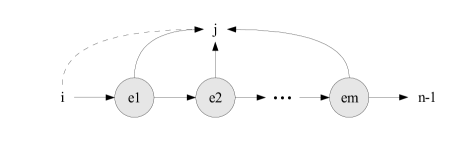
Figure 3: Construction rule for the $\beta$-stopping game $G^{\prime}$ of $G$, where $\beta=1/2^{m}$ and $m=cn$. The dashed edge is present in $G$, but not in $G^{\prime}$; it is replaced by the depicted elements.

Two important properties of the $\beta$-stopping game $G^{\prime}$ have been set forth by Condon:

1. $G^{\prime}$ can be constructed from $G$ in time $O(n^{2})$, where the constant $c$ only has a linear effect on the runtime of the construction algorithm and is hidden in the O-notation.

2. For arbitrary player strategies $\tau$ and $\sigma$, the corresponding value vectors $\vec{v}_{\tau,\sigma}$ of $G$ and ${\vec{v}^{\prime}}_{\tau,\sigma}$ of $G^{\prime}$ satisfy

   $$|v_{\tau,\sigma}(i)-v^{\prime}_{\tau,\sigma}(i)|\leq 2^{n(3-c)}\qquad i\in V$$ (4)

We observe that by choosing $c$ large enough, the differences between corresponding vertex values of the games $G$ and $G^{\prime}$ can be made arbitrarily small, though $G^{\prime}$ can still be constructed in time polynomial in the size of $G$. We will use this result, as well as previous results from this section, for proving the claims we make in the next section.

4 Complexity Survey

We begin this section by showing that – given a simple stochastic game $G$ – the below function problems have polynomial-time equivalent complexities:

1. What is the value of $G$?

2. What is the optimal value vector of $G$?

3. What are optimal player strategies of $G$?

Proof.

“$2\leq_{p}1$”: Let us assume that Algorithm $A1$ computes the value of the game $G$. From $A1$, we construct an Algorithm $A2$ which computes the optimal value vector of $G$. On input of $G$, $A2$ iterates over all vertices $i$ of $G$. In each iteration, $A2$ changes the start vertex of $G$ to be $i$ and then performs a run of $A1$ on $G$, yielding the optimal vertex value $v(i)$. After the last iteration, $A2$ outputs the computed values in form of the optimal value vector of $G$. The runtime of $A2$ is dominated by the queries to $A1$ and since $A2$ makes n queries to $A1$, $A2$ is efficient given $A1$ is.

“$3\leq_{p}2$”: Suppose Algorithm $A2$ computes the optimal value vector of the game $G$. We give an informal description of an Algorithm $A3$ which, using $A2$, computes the optimal player strategies of $G$. Our tool will be the result from the previous section that every min (max) strategy, which is locally optimal at every min (max) vertex of $G$, is an optimal min (max) strategy of $G$; it therefore suffices for $A3$ to compute two locally optimal strategies $\tau_{opt}$ and $\sigma_{opt}$ for the players. On input of $G$, $A3$ runs $A2$ on $G$, yielding the optimal value vector $\vec{v}$ of $G$. For each min vertex $i$ with children $j$ and $k$, $A3$ adds $(i,j)$ to the initial empty $\tau$ if $v(j)\leq v(k)$, else $A3$ adds $(i,k)$ to $\tau$. Similarly, for each max vertex $i$ with children $j$ and $k$, $A3$ adds $(i,j)$ to the initial empty $\sigma$ if $v(j)\geq v(k)$, else $A3$ adds $(i,k)$ to $\sigma$. Following this construction, $\tau_{opt}$ and $\sigma_{opt}$ are locally optimal strategies and since $A3$ makes one query to $A2$ and performs $O(n)$ instructions, $A3$ is efficient given $A2$ is.

“$1\leq_{p}3$”: From an algorithm $A3$ which computes a pair of optimal player strategies of the game $G$, we construct an algorithm $A1$ which computes the value of $G$. On input of $G$, $A1$ runs $A3$ on $G$ to obtain the optimal player strategies $\tau_{opt}$ and $\sigma_{opt}$ of $G$. In time $O(n)$, $A1$ then constructs the reduced game $G_{\tau_{opt},\sigma_{opt}}$ corresponding to $\tau_{opt}$ and $\sigma_{opt}$. We already argued in the previous section that the value vector (and hence the value) of a reduced game can be computed in time polynomial in the size of the game. Since $A1$ makes one call to $A3$, $A1$ is efficient given $A3$ is.∎

SSG-TWOKIND (function)

Input:	Simple stochastic game $G$, lacking one vertex kind
Question:	What is the optimal value vector $\vec{v}$ of $G$?

Complexity class: FP

Algorithms:

Papers discussing algorithms for SSG-TWOKIND include [6, 5, 7, 16, 15, 1]. In the case that $G$ lacks min vertices, SSG-TWOKIND can be expressed as the following linear optimization (or programming) problem, as was first shown by Derman [6]

$$\sum_{i=1}^{n}v(i)\rightarrow\min$$

subject to $v(n-1)=0$, $v(n)=1$ and

$$v(i)\geq\begin{cases}0&1\leq i\leq n\\ v(j)&\text{if }i\text{ is a max vertex with child }j\\ \frac{1}{2}(v(j)+v(k))&\text{if }i\text{ is an average vertex with children }j\text{ and }k\end{cases}$$

Similarly, in the case that $G$ lacks max vertices, Derman showed that the optimal value vector of $G$ is the unique solution to the linear optimization problem

$$\sum_{i=1}^{n}v(i)\rightarrow\max$$

subject to $v(n-1)=0$, $v(n)=1$ and

$$v(i)\leq\begin{cases}0&1\leq i\leq n\\ v(j)&\text{if }i\text{ is a min vertex with child }j\\ \frac{1}{2}(v(j)+v(k))&\text{if }i\text{ is an average vertex with children }j\text{ and }k\end{cases}$$

Khachian [10] was the first to show that linear programming problems can be solved in time polynomial in the bits needed to describe the problem. Since the amount of bits needed to encode any of the above formulas is a polynomial function of $n$ [4], we obtain the fruit that the value vector $\vec{v}$ of $G$ can be computed in polynomial time.

So called interior point algorithms for linear programming problems, which can move through the feasible region instead than just along its boundary, perform best in practice. According to http://en.wikipedia.orgwikipedia, Mehrotra’s [13] interior point algorithm is regarded as the fastest, though a worst case boundary is not available. Up to date, there exists no strongly polynomial time algorithm for linear programming problems, i.e one that is polynomial in the number of variables of the problem up to order ~4.

In the case that $G$ lacks average vertices, the algorithm given in appendix A correctly computes the optimal value vector of $G$. The number of executions of the repeat loop is $O(n)$, as $D$ is static after at most $n-2$ executions. It follows that the algorithm has quadratic runtime, which is a much better result as that obtained for the above linear programming problems.

SSG-OVV (function)

Input:	Simple stochastic game $G$
Question:	What is the optimal value vector $\vec{v}$ of $G$?

Complexity class: FNP

We will first give an informal description of the proof that SSG-OVV$\in FNP$. Let $\Omega_{n}\supset\Omega_{t}$ be a superset of the possible vertex values of $G$, as discussed in (2). The proof is based on the fact that there exists exactly one vector $\vec{z}$ from the set $\Omega_{n}^{n}$ – namely the optimal value vector of $G$ – which satisfies $|z(i)-v^{\prime}(i)|\leq 4^{-2n}/2$ for all $i\in V$, where $\vec{v}^{\prime}$ is the optimal value vector of the $1/2^{9n}$-stopping game $G^{\prime}$ of $G$. We deduce that a nondeterministic Turing-machine $M$ for problem SSG-OVV could guess an arbitrary vector $\vec{z}\in\Omega_{n}^{n}$ and – assuming $M$ knows $\vec{v}^{\prime}$ – argue in polynomial time that $\vec{z}=\vec{v}$ if and only if $\vec{z}$ satisfies the mentioned constraint. Of course, $M$ cannot compute $\vec{v}^{\prime}$ from scratch, but since $M$ is nondeterministic, we can happily let it, next to $\vec{v}$, also guess $\vec{v}^{\prime}$. By evaluating (3), $M$ can easily verify whether its guess of $\vec{v}^{\prime}$ is correct. Therefore, letting $M$ guess the optimal value vectors of both $G$ and $G^{\prime}$, $M$ is able to conduct a polynomial time verification of both guesses.

Considering a formal proof, we first show that the difference between two vertex values of $G$ is either 0 or has a lower bound $\delta$. Let $\alpha,\beta\in\Omega_{n}$. Then either $|\alpha-\beta|=0$ or

$$|\alpha-\beta|=\left|\frac{p}{q}-\frac{p^{\prime}}{q^{\prime}}\right|=\left|\frac{pq^{\prime}-p^{\prime}q}{qq^{\prime}}\right|\geq\frac{1}{qq^{\prime}}\geq\frac{1}{4^{n}4^{n}}=4^{-2n}=:\delta$$

Following (4), we further observe that the differences between corresponding vertex values in the games $G$ and the associated $1/2^{9n}$-stopping game $G^{\prime}$ are bound below $\delta/2$, i. e. for arbitrary strategies $\tau$ and $\sigma$

$$|v_{\tau,\sigma}(i)-{v^{\prime}}_{\tau,\sigma}(i)|\leq 2^{-6n}=4^{-3n}<\delta/2\qquad i\in V$$

On input of $G$, a nondeterministic Turing-machine $M$ for problem SSG-OVV first guesses one vector from the set $\Omega_{n}^{n}$ to be the optimal value vector of $G$ and one vector from the set $\Omega_{n^{\prime}}^{n^{\prime}}$ to be the optimal value vector of $G^{\prime}$, where $n^{\prime}=9n|E|+n$. Let us denote these vectors by the tuple $(\vec{z},\vec{s})$. If we define that $M$ accepts $(\vec{z},\vec{s})$ if $\vec{z}=I_{G}(\vec{z})$, $\vec{s}=I_{G^{\prime}}(\vec{s})$ and $|z(i)-s(i)|<\delta/2$ for all $i\in V$, then $M$ accepts $(\vec{z},\vec{s})$ if and only if $\vec{z}=\vec{v}\wedge\vec{s}=\vec{v}^{\prime}$. Also it should be clear that $M$ comes to a conclusion in time polynomial in the number of vertices of $G$, as in particular $M$ is able to construct $G^{\prime}$ from $G$ in time $O(n^{2})$.

Proof.

Instead of saying “$M$ accepts $(\vec{z},\vec{s})$”, we will just say “$M$ accepts”. “$\Rightarrow$”: If $M$ accepts, $\vec{s}=I_{G^{\prime}}(\vec{s})$ and hence $\vec{s}=\vec{v}^{\prime}$. It remains to prove that if $M$ accepts, $\vec{z}=\vec{v}$ holds. Suppose $M$ accepts but $\vec{z}\neq\vec{v}$. If $\vec{z}\neq\vec{v}$, then $|z(i)-v(i)|\geq\delta$ for at least one $i\in V$. Since $M$ accepts, $|z(i)-s(i)|=|z(i)-v(i)^{\prime}|<\delta/2$ for all $i\in V$. It follows that $|v(i)-v(i)^{\prime}|\geq\delta/2$ for at least one $i\in V$ which contradicts the construction of $G^{\prime}$. “$\Leftarrow$”: Suppose $\vec{z}=\vec{v}$ and $\vec{s}=\vec{v}^{\prime}$. Then obviously $\vec{z}=I_{G}(\vec{z})$, $\vec{s}=I_{G^{\prime}}(\vec{s})$ and $|z(i)-s(i)|<\delta/2$ for all $i\in V$ by construction of $G^{\prime}$. Hence M accepts. ∎

Algorithms:

All algorithms [2, 12, 5, 11, 15, 7, 16] suggested to date for the problem of finding a solution to (3) have exponential time complexities. The most intuitive of those operates on the basis of the iterative update rule $\vec{v}_{i+1}=I_{G}(\vec{v}_{i})$ and is called successive approximation or value iteration algorithm. As already mentioned, this algorithm is guaranteed to converge to the correct solution only if $G$ is stopping. In her paper about algorithms for simple stochastic games, Condon [5] presents a “worst case” example for the successive approximation algorithm in form of a special game graph, where the algorithm takes an exponential number of updates until it finds the optimal value vector.

So called strategy improvement algorithms try to iteratively improve an initial pair of strategies until convergence. A particularly simple algorithm of this class is the one of Hoffman & Karp [11], for which a worst case running time of $O(2^{n}/n)$ is established. Björklund & Vorobyov’s [2] randomized algorithm dating from 2005 has a worst case running time of $O(2^{{}^{\sqrt{n\cdot log(n)}}})$, which as of the authors knowledge, is the best result obtained to date.

SSG-VALUE* (decision)

Input:	Simple stochastic game $G$, $\alpha\in\Omega_{n}$
Question:	Is the value of $G>\alpha$?

Complexity class: $NP\cap coNP$

SSG-VALUE* is a straightforward extension of the SSG-VALUE Problem, which is defined by $\alpha=1/2$. Using the same terminology as for the previous problem, a nondeterministic Turing-machine $M$ for SSG-VALUE* first guesses one vector from the set $\Omega_{n^{\prime}}^{n^{\prime}}$ to be the optimal value vector of the $1/2^{9n}$-stopping game $G^{\prime}$ of $G$, where $n^{\prime}=9n|E|+n$. If we denote this vector by $\vec{s}$ and define that $M$ accepts $\vec{s}$ if $\vec{s}=I_{G^{\prime}}(\vec{s})$ and $s(start)>\alpha$, then $M$ accepts $\vec{s}$ if and only if $value>\alpha\wedge\vec{s}=\vec{v}^{\prime}$. It should also be clear that $M$ comes to a conclusion in time polynomial in the size of $G$.

Proof.

“$\Rightarrow$”: If $M$ accepts $\vec{s}$, then $\vec{s}=I_{G^{\prime}}(\vec{s})$ and therefore $\vec{s}=\vec{v}^{\prime}$. It remains to show that if $M$ accepts $\vec{s}$, $value>\alpha$. Suppose $M$ accepts $\vec{s}$ but $value\leq\alpha$. If $value\leq\alpha$ then $value^{\prime}=s(start)\leq\alpha$ since the stopping game $G^{\prime}$ always has lower value by construction. Hence $M$ cannot accept $\vec{s}$. “$\Leftarrow$”: Suppose $value>\alpha$ and $\vec{s}=\vec{v}^{\prime}$. Then $value\geq\alpha+\delta$ and since, by construction of $G^{\prime}$, $|value-s(start)|\leq\delta/2$, it follows that $s(start)>\alpha$. Since also $\vec{s}=I_{G^{\prime}}(\vec{s})$, M accepts $\vec{s}$. Applying a small modification to $M$ by letting it accept if $s(start)\leq\alpha$, $M$ can obviously also decide the complement of SSG-VALUE* . ∎

Algorithms:

The author is not aware of any algorithm specially tailored for SSG-VALUE*, instead, algorithms for the more general SSG-OVV are used to solve SSG-VALUE*. Though theoretically, algorithms for SSG-VALUE* could exploit the circumstance that – depending on the topology of $G$ – not all optimal vertex values of $G$ would need to be computed in order to solve the problem, as we are mainly concerned with the worst case behavior of such algorithms, the case where the value of $G$ depends on its whole game graph must be assumed. Therefore, the value vector of $G$ must be computed after all.

5 Conclusion and Open Problems

We have seen that the most interesting and also most difficult simple stochastic game problem, that of computing the optimal value vector, is hard to solve. However, restricting the input to simple stochastic games that lack one vertex kind, we observed that the same problem becomes tractable and can be solved rather efficiently. Another result we obtained was that the value vector of reduced games can be computed in polynomial time, i.e that given a simple stochastic game and a pair of player strategies, the question about the winning-probabilities of the players is efficient answerable.

Sadly, we were not able to show polynomial time equivalence of SSG-OVV and SSG-VALUE* but we would still like to know what the decision equivalent of SSG-OVV is. Another major open problem is to show completeness of SSG-VALUE (or SSG-OVV) for a specific complexity class, thereby specifying the problem’s exact complexity. In a last word, Condon expressed the possibility that finding an algorithm that seperates simple stochastic games with low value $(\alpha<0,25)$ from those with high value $(\alpha>0,75)$ might be of significance in solving the master problem: SSG-VALUE $\in P$?

Appendix A

Algorithm 1 optimalValueVector$(G)$

   input simple stochastic game $G=(V,E)$

   output optimal value vector $\vec{v}$ of $G$

   require $V_{avg}=\emptyset$

   begin

   $D=\{n-1,n\},$ $\vec{v}=\vec{0}$

  repeat

     for  $i\in V\setminus D$  do

        if  $i$ is a max vertex with a 1-valued child in $D$  then

            $D=D\cup\{i\},$ $v(i)=1$

        else if  i is a max vertex with two 0-valued children in $D$  then

            $D=D\cup\{i\},$ $v(i)=0$

        else if  i is a min vertex with a 0-valued child in $D$  then

            $D=D\cup\{i\},$ $v(i)=0$

        else if  i is a min vertex with two 1-valued children in $D$  then

            $D=D\cup\{i\},$ $v(i)=1$

        end if

     end for

  until  $D$ is static

   return $\vec{v}$

   end

References

- [1] Daniel Anderson. Improved combinatorial algorithms for mean payoff games. Master’s thesis, University of Upsala, 2006.
- [2] Henrik Björklund and Sergei G. Vorobyov. Combinatorial structure and randomized subexponential algorithms for infinite games. Theoretical Computer Science, 349(3):347–360, 2005.
- [3] Chatterjee, Majumdar, and Jurdzinski. On nash equilibria in stochastic games. In CSL: 18th Workshop on Computer Science Logic. LNCS, Springer-Verlag, 2004.
- [4] A. Condon. The complexity of stochastic games. Information and Computation, 96:203–224, 1992.
- [5] A. Condon. On algorithms for simple stochastic games. DIMACS Series in Discrete Mathematics and Theoretical Computer Science, 13:51–71, 1993.
- [6] Cyrus Derman. Finite State Markovian Decision Processes, volume 67 of Mathematics in Science and Engineering. Academic Press, New York, NY, 1970.
- [7] Jerzy A. Filar, T. A. Schultz, F. Thuijsman, and O. J. Vrieze. Nonlinear programming and stationary equilibria in stochastic games. Math. Program, 50:227–237, 1991.
- [8] Gartner and Rust. Simple stochastic games and P-matrix generalized linear complementarity problems. FCT: Fundamentals (or Foundations) of Computation Theory, 15, 2005.
- [9] Brendan Juba. On the hardness of simple stochastic games. Master’s thesis, Massachusetts Institute of Technology, 2006.
- [10] L. G. Khachian. A polynomial algorithm in linear programming. Soviet Mathematics, 20(191–194), 1979.
- [11] V. S. Anil Kumar and R. Tripathi. Algorithmic results in simple stochastic games. Technical Report TR855, University of Rochester, Computer Science Department, 2004.
- [12] Walter Ludwig. A subexponential randomized algorithm for the simple stochastic game problem. Inf. Comput., 117(1):151–155, 1995.
- [13] S. Mehrotra. On finding a vertex solution using interior point methods. Linear Algebra and its Applications, 152:233–254, 1991.
- [14] L. S. Shalpey. Stochastic games. Proceedings of the National Academy of Sciences, 39:1095–1100, 1953.
- [15] Rafal Somla. New algorithms for solving simple stochastic games. Electr. Notes Theor. Comput. Sci, 119(1):51–65, 2005.
- [16] Csaba Szepesvári and Michael L. Littman. Generalized Markov decision processes: Dynamic-programming and reinforcement-learning algorithms. Technical Report CS-96-11, Brown University, Providence, RI, 1996.